Volume 3, 2018, Pages 1893–1901
HIC 2018. 13th International Conference on Hydroinformatics
Distributed input-delay Model Predictive Control of inland
waterways
P. Segovia
1,2,3, L. Rajaoarisoa
3, F. Nejjari
1, E. Duviella
3, and V. Puig
1,21 Research Center for Supervision, Safety and Automatic Control (CS2AC), Universitat Polit`ecnica de Catalunya
(UPC), Terrassa Campus, Gaia Building, Rambla Sant Nebridi 22, 08222 Terrassa, Spain
{pablo.segovia, fatiha.nejjari, vicenc.puig}@upc.edu
2 Institut de Rob`otica i Inform`atica Industrial (CSIC-UPC), c/ Llorens i Artigas 4-6, 08028 Barcelona, Spain 3 IMT Lille Douai, Univ. Lille, Unit´e de Recherche Informatique Automatique, F-59000 Lille, France
{lala.rajaoarisoa, eric.duviella}@imt-lille-douai.fr
Abstract
Inland waterways are large, complex systems composed of interconnected navigation reaches dedicated mainly to navigation. These reaches are generally characterized by negligible bottom slopes and large time delays. The latter requires ensuring the coordination of the current control actions and their delayed effects in the network. Centralized control strategies are often impractical to implement due to the size of the system. To overcome this issue, a distributed Model Predictive Control (MPC) approach is proposed. The system partitioning is based on a reordering of the optimality conditions matrix, and the control actions are coordinated by means of the Optimality Condition Decomposition (OCD) methodology. The case study is inspired by a real inland waterways system and shows the performance of the approach.
1
Introduction
Certain aspects of the management of modern water systems require advanced control methods [4]. For this reason, Model Predictive Control (MPC) is applied in the present work. This methodology is very well suited in those cases where the future references are known. Roughly speaking, reference values are the desired water levels in the reaches, while lock operations that allow boats to cross from one reach to the next one are regarded as disturbances. Gates are used to dispatch water along the system so that the control objectives are satisfied and the disturbances are rejected.
The framework of decentralized and distributed predictive control of water systems has attracted considerable interest in the past years. A decentralized adaptive predictive controller for irrigation canals was designed in [5], aiming at controlling the downstream water levels of a set of reaches. An optimal decentralized control architecture was presented in [6] to ensure the efficient management of an inland navigation network in a global change context. Another decentralized controller was designed in [7] for a part of a real inland navigation network with a distributary. The application of non-centralized approaches to drinking water networks to improve the performance with respect to the centralized coun-terpart was discussed in [8]. A comparison of decentralized and distributed control strategies for irriga-tion systems was performed in [9], where the benefits of cooperative distributed control were validated. A hierarchical distributed MPC approach applied to irrigation canal planning was presented in [10], addressing a risk management strategy.
Summary of the paper and contributions
The centralized MPC scheme presented in [11] might not be practical to implement in the case of large-scale systems due to the spatial distribution of the network. To overcome this limitation, this work proposes a distributed MPC approach based on the initial centralized design. The formulation and manipulation of the Karush-Kuhn-Tucker (KKT) centralized matrix yields separable KKT subsystems, which define the structure of the decomposed control sub-problems [12]. Once this decomposed struc-ture is attained, the Optimality Condition Decomposition (OCD) technique [13] is used to obtain the consensus strategy that leads to the best global performance. The rest of the paper is organized as fol-lows: Section 2 summarizes the centralized MPC formulation presented in the aforementioned work. In Section 3, the centralized KKT system is formulated, and it is shown how to manipulate it to obtain the distributed KKT system. Furthermore, the OCD technique is presented, and the final distributed MPC formulation is given. An illustrative case study, inspired by part of a real inland waterways network, is presented in Section 4, which illustrates the proposed approach and highlights the performance of the control strategy. Section 5 draws conclusions and outlines future steps.
Notation
Throughout this paper, letRn denote the set of column real vectors of lengthn. Scalars are denoted
with either lowercase or uppercase letters (e.g. α,a,A, etc.); vectors, with bold lowercase letters (e.g. a
aa,bbb, etc.); and matrices, with bold uppercase letters (e.g. AAA,BBB, etc.). Furthermore, all vectors are column vectors unless otherwise stated, and 000 denotes a zero column vector of suitable dimensions. Transposition is denoted with the superscript|, and the operators<,≤,=,≥and>denote element-wise relations of vectors.
2
Centralized MPC formulation
2.1
IDZ model and equivalent state-space formulation
In order to develop an MPC for inland waterways, a model that describes the dynamic behavior of the system is needed. The Saint-Venant (SV) differential equations can accurately describe the real dynamics of the system [14]. However, these equations are not well suited for control purposes as they have no known analytical solution and are very sensitive to errors in the parameters. Many simplified models have been proposed to deal with these issues; among all of them, the Integral Delay Zero (IDZ) model [15] is used in this work. The general IDZ input-output expression that links the discharges and the water depths at the boundaries of a reach is given by:
"
y(0,s)
y(L,s)
# =
"
p11(s) p12(s)
p21(s) p22(s)
#
| {z }
P
"
q(0,s)
q(L,s)
#
, (1)
where 0 andLare the abscissas for the initial and final ends of the canal;y(0,s)andy(L,s), the upstream and downstream water levels; q(0,s)andq(L,s), the upstream inflow and downstream outflow; and
pi j(s) =
αi j·s+1 Ai j·s e
−τi j·s, the different terms of the IDZ model (A
i j is the integrator gain,τi j is the time
delay andαi jis the inverse of the zero). The parameters of the first equation of (1) are linked to the
upstream water level, while those in the second equation are linked to the downstream water level. Based on this, the notation of the parameters is modified in [15] and is adopted in the present work:
A11=A12=Au,A21=A22=Ad,τ12=τuandτ21=τd(τ11=τ22=0).
An equivalent discrete state-space formulation is obtained to ensure the correct coordination between actual control values and their delayed effect in the system (a sampling periodTsis used):
xxxk+1=
"
1 0
0 1
#
xxxk+
"
Ts 0
0 Ts #
u
uuk+
"
0 Ts
Ts 0
#
uuuk−n; yyyk=
"1 Au 0
0 A1
d #
xxxk+
"α11
Au 0
0 α22
Ad #
uuuk+
"
0 α12
Au
α21
Ad 0 #
u
uuk−n
(2) withkthe discrete-time instant anduuuk−nthe input vector delayednsamples (n=dτ/Tse, withd·ethe
ceiling function). In practice, the numerical values ofτdandτuare almost the same, leading to a single
value ofn. Equation (2) describes a reach with two inputs and two outputs. The formulation of a system withnxstates,nuinputs andnyoutputs, and with demandsdk(acting as additive disturbances), is:
xxxk+1=AAAxxxk+BBBuuuuk+BBBu−nuuuk−n+BBBddddk+BBBd−ndddk−n; yyyk=CCCxxxk+DDDuuuuk+DDDu−nuuuk−n+DDDddddk+DDDd−ndddk−n
(3)
2.2
Control design
The main principle of MPC techniques resides in computing a control sequence that makes the pre-dicted response move to the setpoint in an optimal manner without violating the constraints. Thus, it is necessary to define the constraints and the operational goals to be fulfilled. The system functioning is constrained by the physical nature of the variables as well as some elements in the waterways. Each of the constraints is described and formulated below:
• Mass balance relations must be imposed at the nodes: 000=EEEuuuuk+EEEddddk.
• The lower and upper bounds of them-th actuator must be respected:uuum≤uuum k ≤uuu
m, m=1, ...,N m,
withNmthe total number of actuators in the system.
• The water levelsyyykmust be kept within the predefined navigation interval h
y
r,yr i
to ensure the navigability:yyy
Furthermore, the several operational goals that are to be fulfilled are the following:
• Maintain the water levels close to the setpointsyyyr:Jk1= (yyyk−yyyr)|(yyyk−yyyr).
• Reduce the economic cost derived from the operation of the available controlled equipment:Jk2=
γγγuuu|kuuuk.
• Guarantee a smooth control action:Jk3=∆uuu|k∆uuuk.
• Penalize the relaxation of the navigability condition to be as little as possible outside the naviga-tion interval:Jk4=ααα|kαααk.
The objectives are gathered to build the objective functionJ= Hp
∑
k=1 4
∑
j=1
βjJkj, with whereHpis the
pre-diction horizon and the weightsβjare selected as shown in [11]. The solution of the centralized control
problem is then given by:
min J (4a)
subject to:
xxxk+i+1|k=AxxxAA k+i|k+BBBuuuuk+i|k+BBBu−nuuuk+i−n|k+BBBddddk+i|k+BBBd−ndddk+i−n|k (4b)
yyyk+i|k=CxxxCC k+i|k+DDDuuuuk+i|k+DDDu−nuuuk+i−n|k+DDDddddk+i|k+DDDd−ndddk+i−n|k (4c)
0
00=EEEuuuuk+i|k+EEEddddk+i|k (4d)
u
uum≤uuumk ≤uuum (4e)
yyy
r−αααk≤yyyk≤yyyr+αααk (4f)
α
ααk≥000 (4g)
withHpthe prediction horizon,ithe time instant along the prediction horizon,kthe current time instant
andk+i|kthe time instantk+igivenk.
3
Distributed MPC formulation
As it has been stated before, centralized control approaches for large-scale systems are often difficult to implement, mainly due to the spatial distribution of the elements in the network. To overcome this limitation, the system is partitioned into sub-systems. In this work, this decomposition step is carried out by manipulating the centralized Karush-Kuhn-Tucker (KKT) matrix of the large-scale problem, which yields separable KKT subsystems that define the structure of the decomposed sub-problems. Once such a decomposed problem structure is obtained, the Optimality Condition Decomposition (OCD) technique is used to coordinate the local controllers to guarantee the best global performance.
3.1
Centralized and distributed KKT systems
To formulate the centralized KKT system, it is necessary first to define the Lagrangian function
L(uuu,yyy,λ1,λ2,λ3) = f(uuu,yyy) +
Hp
∑
j=1
λ1hhh(j1)(uuu,yyy) +λ2hhh(j2)(uuu,yyy) +λ3hhh(j3)(uuu,yyy)
where f(uuu,yyy)is the objective function given in (4a); λ1,λ2andλ3are the Lagrange multipliers; and
h(j1),h(j2)andh(j3)are the three first constraints of the optimization problem (4), respectively. Indeed, the bounds on the variables do not affect the decomposition, and hence they are not considered in this step. Note that the temporal dependence of u and y is not explicitly indicated for readability.
The KKT matrix for the overall system is built using (5), which can be obtained by applying the pri-mal dual interior point method or the gradient-based method [16]. This matrix represents the optimality conditions and is denoted withKKTKKTKKTcent. The next step consists in manipulating this matrix such that a
block-diagonal structure is attained. A number of methods can be employed to transform a symmetric matrix such asKKTKKTKKTcentinto the block-diagonal form. However, some of them are not well suited for the
largeKKTKKTKKTcentmatrices that result from the MPC problem, while others compromise the coupling
infor-mation due to the elimination of some matrix coefficients. The Cuthill-McKee ordering algorithm [17] performs row/column permutation operations in symmetric matrices to obtain a block-diagonal matrix with minimal couplings. This reordering provides as a solutionlKKT block matrices on the diagonal, which can be regarded asl subsystems into which the overall system can be decomposed. The final block-diagonal matrix is denoted withKKTKKTKKTdist.
3.2
Optimality Condition Decomposition
Once the system partitioning has been performed, the local controllers must be designed, and their actions coordinated. The OCD technique decomposes the centralized problem inl sub-problems, and the constraints are decomposed into l groups of constraints, each of them describing the dynamics of a subsystem and the interactions with the rest of subsystems. At each iteration, the method fixes, for the
i-th sub-problem, all variables to their last computed values (denoted in (6) with a tilde), except for the
i-th group of variables. Thelparallel sub-problems are given by
min
u uui,yyyi
(
f(uuu˜1,yyy˜1, . . . ,uuui,yyyi, . . . ,uuu˜l,yyy˜l) + l
∑
j=1,j6=i˜
λjhj(uuu˜1,yyy˜1, . . . ,uuui,yyyi, . . . ,uuu˜l,yyy˜l) )
(6)
subject to:
hi(uuu˜1,yyy˜1, . . . ,uuui,yyyi, . . . ,uuu˜l,yyy˜l) =0 ; uuumi ≤uuumi ≤uuuim; yyyr−αααi≤yyyi≤yyyr+αααi; αααi≥000
Once the solution has been computed for each sub-problem, the Lagrangian multipliers are updated, following, for instance, a sub-gradient technique:λi(ν+1)=λi(ν)+χhi, withνthe current iteration and
χ∈(0,1)a suitable constant. The coordination of the global problem is achieved through the Lagrange multipliers. On the other hand, the convergence speed is characterized by the accepted variation of the values of the multipliers between consecutive iterations.
4
Case study
The result of applying the distributed MPC given by the solution of (6) is presented in this section. The system is first described, then the experimental design is presented, and finally the results are shown and the controller performance is discussed.
4.1
System description
N1
N3 N2
Bif
(1)
(2) (3)
u u
u u
u
Bif Bif
Bif (1)
(2)
(3)
N2
N4 (2) uN2(4)
uN4
(4)
N1
uN3
Figure 1: Scheme of the case study system
gates that allow dispatching water to fulfill the control objectives, as well as locks used by boats to cross from one reach to the adjacent one. Bi f stands for bifurcation, where a gate is used to regulate the flow supplied to reaches 2 and 3. Four identical reaches with the following magnitudes make up the system:L= 27000m(length of the reach),wr =50m(bottom width),mr = 0 (side slope of the reach,
mr= 0 for a rectangular cross section),sb= 0 (bottom slope,sb= 0 for a flat reach),nr = 0.035sm−1/3
(Manning roughness coefficient) andQs= 0.6m3s−1(operating point considered in the SV equations
linearization). The navigability condition is ensured if the water levels are kept in the interval 3.8± 0.1m. However, this objective is disturbed by lock operations with magnitudes: 18000m3(N1), 18000
m3(N2), 9000m3(N3) and 24000m3(N4), with an average duration of 20minin all cases. In each operation, the corresponding water volume is withdrawn from the upstream reach and released into the downstream reach. Thus, the sign of these uncontrolled discharges will depend on whether these nodes are upstream or downstream nodes, i.e. on the system partitioning. In addition, the lock operation time-series model is considered to be known in advance. Indeed, a common waterways management policy dictates that, when a boat passes through a lock, its manager informs the manager of the next lock so that the arrival time of the boat can be anticipated.
4.2
Experimental design
First, the centralized representation (4) is computed for the system depicted in Fig. 1. A sampling timeTs = 20min is considered. The bounds on the gates are±60m3s−1. Next, the decomposition
techniques presented in Section 3.1 are applied to the centralized model. As a result,KKTKKTKKTdist is formed
by two blocks, which indicates that the overall system can be decomposed into two subsystems. The first subsystem (SS.1) comprises reaches 1, 2 and 3, while the second one (SS.2) is only formed by reach 4. The only existing coupling is the input at node N2 (all the water withdrawn from reach 2 is released in reach 4). There is no coupling in the state at N2 as the gate allows different upstream and downstream water depths. Due to lack of space, neitherKKTKKTKKTcentnorKKTKKTKKTdist are presented. A 24-hour navigation
5 6 7 8 9 10 11 12 13 14 15 16 17 18 19 20 21 22 23 241 2 3 4 5 0
5 10 15
dN1
[
m
3/s
]
5 6 7 8 9 10 11 12 13 14 15 16 17 18 19 20 21 22 23 241 2 3 4 5 -15 -7.5 0 7.5 15 dN 2 [ m 3/s ]
5 6 7 8 9 10 11 12 13 14 15 16 17 18 19 20 21 22 23 241 2 3 4 5 -7.5 -5 -2.5 0 dN 3 [ m 3/s ]
5 6 7 8 9 10 11 12 13 14 15 16 17 18 19 20 21 22 23 241 2 3 4 5 -20 -15 -10 -5 0 Time [h] dN 4 [ m 3/s ]
Figure 2: Lock operation profile (solid: disturbances in SS.1; dash-dot: disturbances in SS.2)
4.3
Results
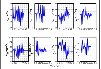
The presented scenario is simulated, and the set of controlled actions and the predicted water levels are depicted in Fig. 3and4, respectively. Since there exists a proportionality between states and outputs (defined by matrixCCC), the states are not depicted. Note also that there are three variables forBi f and two for N2: the distinction is made by adding the reach number after the variable name.
5 8 1114172023 2 5 30 34 38 42 46 UN 1 [m 3/s ]
5 8 1114172023 2 5 -50 -46 -42 -38 -34 -30 UB if ( 1 ) [m 3/s ]
5 8 1114172023 2 5 -50 -46 -42 -38 -34 UB if ( 3 ) [m 3/s ]
5 8 1114172023 2 5 36 40 44 48 UN 3 [ m 3/s ] Time [h] 5 8 1114172023 2 5 -10 -5 0 5 10 UB if ( 2 ) [m 3/s ]
5 8 1114172023 2 5 -46 -42 -38 -34 UN 2 ( 2 ) [m 3/s ]
5 8 1114172023 2 5 34 38 42 46 UN 2 ( 4 ) [m 3/s ]
5 8 1114172023 2 5 -60 -52 -44 -36 -28 UN 4 [ m 3/s ]
Figure 3: Controlled inputs computed by the distributed MPC
5 8 1114172023 2 5 3.6 3.7 3.8 3.9 4 YN 1 [ m ]
5 8 1114172023 2 5 3.6 3.7 3.8 3.9 4 YB if ( 1 ) [m ]
5 8 1114172023 2 5 3.6 3.7 3.8 3.9 4 YB if ( 3 ) [m ]
5 8 1114172023 2 5 3.6 3.7 3.8 3.9 4 YN 3 [ m ] Time [h] 5 8 1114172023 2 5 3.6 3.7 3.8 3.9 4 YB if ( 2 ) [m ]
5 8 1114172023 2 5 3.6 3.7 3.8 3.9 4 YN 2 ( 2 ) [m ]
5 8 1114172023 2 5 3.6 3.7 3.8 3.9 4 YN 2 ( 4 ) [m ]
5 8 1114172023 2 5 3.6 3.7 3.8 3.9 4 YN 4 [ m ]
Figure 4: Levelsyyykkk (blue solid), navigation
intervals (red dash-dot) and setpointsyyyrrr (gray
dashed)
The simulation starts at 5 a.m., one hour before the navigation period. After this period ends (during which the system is disturbed), the water levels return to their equilibrium values. Figure4shows that the distributed MPC is able to keep the levels inside the navigation interval in the presence of disturbances. Note that the absolute values of the control signals in Fig. 3are exactly the same for the two inputs at node N2, where an input coupling exists (different sign due to the sign criterion). Furthermore, the set of control actions is kept within the equipment design range. However, one of the operational goals consisted in guaranteeing a smooth control signal by minimizing∆∆∆uuuk. Although the control signals do
not exhibit the smoothest behavior, the differences between two consecutive control actions are not so large compared to the operational range. This fact should result in a long lifespan of the equipment.
To quantify the controller performance, consider the tracking indices (7) defined as the error between
the predicted levelsyyyk and the setpointsyyyr, with 12
yyyr−yyy
r
lowest TE index is 97.7%, showing that this approach provides satisfactory results and that the tracking performance is guaranteed (TE=100% corresponds to the perfect tracking performance).
T E[%] =100∗
1−
1
Hp
v u u u t
Hp
∑
k=1
yyyk−yyyr
1 2
yyyr−yyy
r
2
(7)
5
Conclusions
This work proposed a distributed MPC approach to keep the levels of inland waterways within the limits in the presence of disturbances created by lock operations. The original centralized problem was presented and divided in sub-problems by manipulating the KKT centralized matrix. As a result, separate sub-problems were obtained, and each of them was taken care of by a local controller. The OCD technique was used to coordinate the controllers to obtain the best global performance. This approach proved to perform well, as it was shown by means of the case study. Thus, it can be stated that this methodology constitutes an efficient approach for large-scale systems, for which the centralized counterparts are difficult to implement due to the spatial distribution of the elements in the network.
In future works, the effect of possible sensor and actuator faults will be addressed. Therefore, fault-tolerant control techniques using the presented distributed MPC approach will be considered.
Acknowledgements
This work is partially funded by AGAUR of Generalitat de Catalunya through the Advanced Control Systems (SAC) group grant (2017 SGR 482).
References
[1] D. Barcelli, C. Ocampo-Mart´ınez, V. Puig, and A. Bemporad. Decentralized model predictive control of drinking water networks using an automatic subsystem decomposition approach.IFAC Proceedings Volumes, 43(8):572–577, 2010.
[2] D. D. Siljak.Decentralized control of complex systems. Courier Corporation, 2011.
[3] R. Negenborn, P. J. van Overloop, T. Keviczky, and B. De Schutter. Distributed model predictive control of irrigation canals.Networks and Heterogeneous Media, 4(2):359–380, 2009.
[4] P. J. Van Overloop.Model predictive control on open water systems. IOS Press, 2006.
[5] S. Sawadogo, R. Faye, and F. Mora-Camino. Decentralized adaptive predictive control of multireach irrigation canal.International Journal of Systems Science, 32(10):1287–1296, 2001.
[6] L. Rajaoarisoa, K. Horv´ath, E. Duviella, and K. Chuquet. Large-scale system control based on decentralized design. Application to Cuinchy Fontinette Reach.IFAC Proceedings Volumes, 47(3):11105–11110, 2014. [7] P. Segovia, L. Rajaoarisoa, F. Nejjari, V. Puig, and E. Duviella. Decentralized control of inland navigation
networks with distributaries: application to navigation canals in the north of France. In2017 American Control Conference (ACC), pages 3341–3346, May 2017.
[8] J. M. Grosso, C. Ocampo-Mart´ınez, and V. Puig. Non-centralized predictive control for drinking-water sup-ply systems. InReal-time Monitoring and Operational Control of Drinking-Water Systems, pages 341–360. Springer, 2017.
[10] A. Zafra-Cabeza, J. M. Maestre, M. A. Ridao, E. F. Camacho, and L. S´anchez. A hierarchical distributed model predictive control approach to irrigation canals: a risk mitigation perspective. Journal of Process Control, 21(5):787–799, 2011.
[11] P. Segovia, L. Rajaoarisoa, F. Nejjari, V. Puig, and E. Duviella. Input-delay model predictive control of inland waterways considering the backwater effect. In2nd IEEE Conference on Control Technology and Applications, to appear.
[12] T. Darure. Contribution to Energy Optimization for Large-scale Buildings: An Integrated approach of diag-nosis and economic control with moving horizon. PhD thesis, Universit´e de Lorraine, 2017.
[13] A. J. Conejo, E. Castillo, R. M´ınguez, and R. Garc´ıa-Bertrand. Decomposition techniques in mathematical programming: engineering and science applications. Springer Science & Business Media, 2006.
[14] V. T. Chow.Open-channel hydraulics. McGraw-Hill Book Co. Inc, New York, 1959. [15] X. Litrico and V. Fromion.Modeling and Control of Hydrosystems. Springer, 2009. [16] S. Boyd and L. Vandenberghe.Convex optimization. Cambridge university press, 2004.