Volume 60, 2019, Pages 15–26
Proceedings of 11th International Conference on Bioinformatics and Computational Biology
gcn.MOPS: Accelerating cn.MOPS with GPU
Mohammad Alkhamis and Amirali Baniasadi
[email protected]
[email protected]
University of Victoria, Victoria, British Columbia, Canada
Abstract
cn.MOPS is a frequently cited model-based algorithm used to quantitatively detect copy-number variations in next-generation, DNA-sequencing data. Previous work has im-plemented the algorithm as an R package and has achieved considerable yet limited perfor-mance improvement by employing multi-CPU parallelism (maximum achievable speedup was experimentally determined to be 9.24). In this paper, we propose an alternative mech-anism of process acceleration. Using one CPU core and a GPU device in the proposed solution, gcn.MOPS, we achieve a speedup factor of 159 and reduce memory usage by more than half compared to cn.MOPS running on one CPU core.
1
Introduction
The introduction of next-generation sequencing (NGS) technologies in 2005 has enabled sci-entists and researchers to sequence DNA samples at a relatively low cost. Since 2007, the sequencing cost per genome has dropped at a significantly steeper rate than that projected by
Moore’s law [3]. This made DNA sequencing (DNA-seq) more accessible, which subsequently
led to an explosive growth in the amount of DNA-seq data [5]. One major area of study which benefits from such growth in data is the detection of copy-number variations (CNV) from NGS data using statistical and quantitative methods. Many software tools and algorithms were pioneered [6] to tackle the problem of CNV detection. One of these tools is “Copy Number estimation by a Mixture Of PoissonS” (cn.MOPS) [2]. However, one factor that is limiting cn.MOPS, as well as other software tools in this field, is the computation time of analyzing massive NGS data sets.
While cn.MOPS can accelerate data processing using multiple central processing units (CPU), there is a limit to the maximum achievable speedup due to parallelism overhead. To achieve a speedup that is considerably higher than the maximum offered by multi-CPU paral-lelism, we propose an alternative approach of acceleration. Our approach stems from the notion that cn.MOPS applies the same algorithm on a large amount of independent data elements. Therefore, it is well-suited for execution on a processor that implements the single-instruction-multiple-data architecture (SIMD) such as graphical processing units (GPUs).
of the pipeline, which is the result of the postprocessing step, is minimized by making its ex-ecution time negligible and reducing its memory footprint. In cn.MOPS, the postprocessing step was implemented in a way that effectively resulted in having two copies of the same data in memory. Meanwhile, the techniques used in the GPU-accelerated cn.MOPS (gcn.MOPS) produced results from the modelling step that did not require postprocessing.
In summary, the contributions of this work are:
• Re-architecturing cn.MOPS to suit execution on GPU;
• Accelerating the modelling step by a factor of ∼159×compared to the
experimentally-determined maximum speedup of∼9.24×with multi-CPU parallelism, and;
• Reducing the memory footprint of the postprocessing step by more than a half.
To the best of our knowledge, this paper is the first to propose the use of SIMD processors, i.e. GPUs, to accelerate cn.MOPS and reduce its memory footprint.
2
Max Speedup with multi-CPU Parallelism
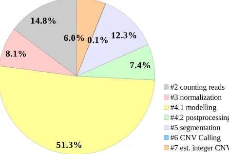
In order to determine the maximum speedup that cn.MOPS can achieve, a sufficiently large, yet relatively small, benchmark is run and profiled. Details about this benchmark which is called BM-A, as well as the used platform, are elaborated in Section 5.2. The total execution time using 1× CPU core is found to be ∼112 minutes. This total does not include the execution time of stage 1, which is mainly loading BAM files from disk. Figure1shows a breakdown of the execution time for each pipeline stage as a percentage of total. Apparently, stage 4, i.e. the modelling and the postprocessing steps combined, is the bottleneck.
14.8%
8.1%
51.3%
7.4% 12.3% 0.1% 6.0%
#2 counting reads #3 normalization #4.1 modelling #4.2 postprocessing #5 segmentation #6 CNV Calling #7 est. integer CNV
Figure 1: Execution time expressed as % of total execution time (∼112 minutes) using 1×CPU core to run benchmark BM-A. The leading numbers in the legend indicates the order of the stage in the execution pipeline. For simplicity, stage #1, which is loading BAM files from disk, is not shown
cn.MOPS in terms of performance, the maximum speedup, ψCP U
max, that can be achieved with
cn.MOPS is estimated.
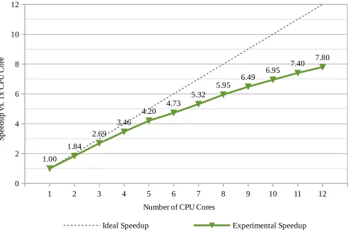
Estimating ψmaxCP U is done by experimentally obtaining the speedup curve, which is shown
in Figure2. For simplicity, the performance is modelled as a polynomial by extrapolating data from Figure2using LibreOffice Calc. The obtained speedup formula,g(p), is shown in Equation 1, where pis the number of processors, i.e. CPU cores.
g(p) =−0.022695p2+ 0.908861p+ 0.141837 (1)
Next, the global maxima forg(p) is found by derivingg(p) and solving the derivative forpsuch that g0(p)=0. This yielded p=20, which meant that ψCP Umax will be achieved using 20× CPU cores. Substitutingp=20 in Equation1yieldedg(20) =ψCP Umax '9.24. In subsequent sections,
we introduce gcn.MOPS which showed significantly higher speedups.
1 2 3 4 5 6 7 8 9 10 11 12 0
2 4 6 8 10 12
1.00 1.84
2.69 3.46
4.20 4.73 5.32
5.95 6.49
6.95 7.40 7.80
Ideal Speedup Experimental Speedup Number of CPU Cores
Sp
ee
du
p
vs
. 1
x
C
PU
C
or
e
Figure 2: Speedup curve for multi-CPU parallelism for the modelling step
3
Overview of cn.MOPS
The basic idea behind cn.MOPS is that a CNV is detected in a given chromosomal segment for a given DNA-seq sample if the following conditions hold:
1. variation in read counts (RCs) is detected across samples for a given chromosomal segment;
2. variation in RCs is detected across chromosomal segments for a given sample.
Analysis for the second condition happens in the segmentation step, which is beyond the scope of this paper. Meanwhile, analysis for the first condition takes place in the modelling step, which is the focus of this paper, and, hence, is briefly explained.
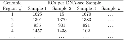
Analysis for the first condition begins by forming an RC matrix whose rows contain the RC
of multiple DNA-seq samples for a single genomic segment. Table 1 shows an example of an
RC matrix. For each row in the RC matrix, cn.MOPS computes multiple values as follows:
Genomic RCs per DNA-seq Sample
Region # Sample 1 Sample 2 Sample 3 Sample k
1 1625 15 1670 . . .
2 1391 1379 1383 . . .
3 935 901 921 . . .
4 1457 1438 102 . . .
. . . .
Table 1: An example of an RC matrix, where a genomic region represents a genomic range
Equation2.
I/NI = 1
N N X k=1 n X i=0 ˆ
αik× |log(i/2)| (2)
• The posterior matrix (αˆ): the probability distribution of RCs xk for samples 1..N
cor-responding to copy number (CN) i. Matrix values are calculated as shown in Equation
3, where: P is the probability density of Poisson distribution; and the denominator is a conditional probability.
ˆ
αik=
αold
i ×P(xk;2iλold)
p(xk;αold, λold)
(3)
• Vector αnew: a model parameter which is calculated using Equation 4, where: initial
valuesαold
i are set to 0.05 exceptαold2 which is set to 0.6;γi is related to the Drichet prior
onαi; and γs=P n i=0γi.
αnewi =
1 N
PN
k=1αˆik+ 1
N(γi−1)
1 + N1(γs−n)
(4)
• λnew: the expected read count for CN2 which is calculated using Equation5.
λnew=
1 N
PN
k=1xk
Pn i=0 i 2N PN
k=1αˆik
(5)
• “The signed individual I/NI” (sI/NI): measures the contribution of each sample to the I/NI call and whether that contribution is a gain or a loss. This vector is used by the segmentation algorithm to join consecutive, I/NI-calling, GRs into a CNV chromosomal segment. Values in this vector are calculated using Equation 6, which is similar to the inner summation of Equation2 without taking the absolute value of the log function.
sI/NI =
n
X
i=0
ˆ
αik×log(i/2) (6)
• The expected copy number (CN): each component in this vector corresponds to a sample such that components are row-labels of the maximum value in each column ofαˆ.
for relatively large data sets. Therefore, these equations are accelerated in our method. It should be noted that said values are set to constants if all read counts across samples for a genomic region are less then a given threshold, i.e. minimum read count (MRC). Experimentally, such an operation is memory-intensive if executed on GPU. Thus, accelerating it is handled differently as presented in sections4.4and4.5.
4
Accelerating cn.MOPS Using GPU
In order to accelerate with GPU and CUDA, fundamental changes to the existing code and algorithms are often required. For instance, cn.MOPS utilizes R’s functional primitive ”apply()” to invoke its core algorithm on multiple data elements. While simple and convenient, this primitive is replaced with a conventional for-loop that is executed in C/C++ instead of in R. This is done in order to make it possible to efficiently offload work to GPU. Potentially, there can be a speedup gain by executing this loop in C/C++, which we do not measure and report here. The rest of this section presents the employed techniques which collectively results in significantly better performance compared to cn.MOPS.
4.1
Assigning Memory To GPU Threads
Threads are assigned logical partitions of three, separately allocated, GPU memory spaces: the input matrix, the result buffer, and the draft space used for intermediate calculations. Since there is no dependency between rows in an input matrix, each GPU thread can independently handle a single row. It should be noted that the number of rows can be greater than the maximum allowed number of threads in a kernel launch (the grid). Thus, multiple rows of the input matrix are assigned to each thread in the kernel which are separated by a stride of length
g, i.e. the number of threads in the grid, as shown in Table2.
Thread ID iteration 0 . . . iterationi
thread 0 row 0 . . . row i×g
thread 1 row 1 . . . row i×g + 1
thread 2 row 2 . . . row i×g + 2
thread 3 row 3 . . . row i×g + 3
..
. ... . .. ...
thread g-1 row g-1 . . . row (i+1)×g -1
Table 2: Illustration of the grid-strided loop for a grid of sizeg
In addition, the number of rows can be greater than what GPU memory can accommodate. Again, there is no dependency between rows of an input matrix. Accordingly, the input matrix is partitioned into smaller chunks such that each chunk fits in GPU memory. Then, the kernel is launched multiple times to process each chunk independently.
4.2
Coalescing Memory Accesses
Ensuring a software design, in which threads are arranged to make coalesced access to data,
can positively impact performance. For instance, if thread T makes a memory-read request
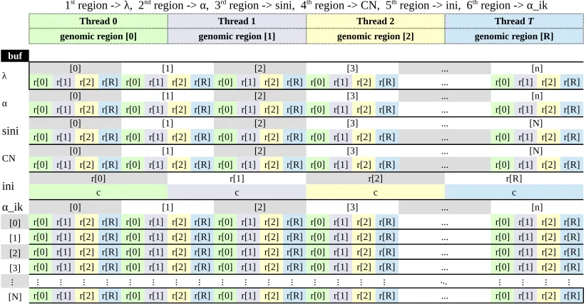
threadT also request neighbours of $addr, then no further memory transactions are executed since data requested by neighbours ofT are already loaded. The performance impact in this case is that less memory transactions are executed to service multiple threads. Since global memory transactions have high latency, minimizing them results in a performance improvement. If memory access patterns are inherited from cn.MOPS, memory requests for elements in the result buffer will be strided and, hence, uncoalesced as shown in Figure3, wheren is the number of classes andN is the number of samples. This is confirmed by running our benchmark, which is detailed in Section5.2, to obtain metrics “global memory load efficiency” and “global memory store efficiency” [4]. The values for these two metrics are 9.2% and 25%, respectively. These considerably low percentages suggested that memory bandwidth is wasted as most of the elements loaded from global memory are unused.
Logical labels and coloring (i.e. not part of buffer data)
Thread 0 Thread 1 Thread 2
genomic region [0] genomic region [1] genomic region [2] genomic region [R]
buf
λ [0] [1] [2] [3] ... [n] [0] [1] [2] [3] ... [n] [0] [1] [2] [3] ... [n] [0] [1] [2] [3] ... [n]
α [0] [1] [2] [3] ... [n] [0] [1] [2] [3] ... [n] [0] [1] [2] [3] ... [n] [0] [1] [2] [3] ... [n]
sini [0] [1] [2] [3] ... [N] [0] [1] [2] [3] ... [N] [0] [1] [2] [3] ... [N] [0] [1] [2] [3] ... [N]
CN [0] [1] [2] [3] ... [N] [0] [1] [2] [3] ... [N] [0] [1] [2] [3] ... [N] [0] [1] [2] [3] ... [N]
ini c c c c
α_ik [0,0] [0,1] [0,2] [0,3] ... [0,n] [0,0] [0,1] [0,2] [0,3] ... [0,n] [0,0] [0,1] [0,2] [0,3] ... [0,n] [0,0] [0,1] [0,2] [0,3] ... [0,n] [1,0] [1,1] [1,2] [1,3] ... [1,n] [1,0] [1,1] [1,2] [1,3] ... [1,n] [1,0] [1,1] [1,2] [1,3] ... [1,n] [1,0] [1,1] [1,2] [1,3] ... [1,n] [2,0] [2,1] [2,2] [2,3] ... [2,n] [2,0] [2,1] [2,2] [2,3] ... [2,n] [2,0] [2,1] [2,2] [2,3] ... [2,n] [2,0] [2,1] [2,2] [2,3] ... [2,n] [3,0] [3,1] [3,2] [3,3] ... [3,n] [3,0] [3,1] [3,2] [3,3] ... [3,n] [3,0] [3,1] [3,2] [3,3] ... [3,n] [3,0] [3,1] [3,2] [3,3] ... [3,n] .. .. .. .. .. .. .. .. .. .. .. .. .. .. .. .. .. .. .. .. [N,0] [N,1] [N,2] [N,3] ... [N,n] [N,0] [N,1] [N,2] [N,3] ... [N,n] [N,0] [N,1] [N,2] [N,3] ... [N,n] [N,0] [N,1] [N,2] [N,3] ... [N,n]
1st region -> λ, 2nd region -> α, 3rd region -> sini, 4th region -> CN, 5th region -> ini, 6th region -> α_ik
Thread T
... ... ... ...
Figure 3: Memory access patterns for the result buffer inherited from cn.MOPS, wherenis the number of classes,N is the number of samples,Ris the number of genomic regions, andcis a constant. Vertical segments of the same colour indicate a separate logical division within the buffer that is allocated for an indvidual genomic region and, hence, a GPU thread. Darker colors indicate a memory operation for a single iteration, where parallel reads occur across multiple genomic regions only. All simultaneous memory accesses are for reading or writing a single cell in a designated region of the buffer allocated for the variables of each individual genomic region. The whole buffer is contiguous in memory and the order of placement in memory for each variable is the same as shown in the Figure, i.e. λfollowed byαetc.. It should be noted thatR could be larger thanT as explained in section4.1
Logical labels, indexing, and coloring (i.e. not part of buffer data)
Thread 0 Thread 1 Thread 2
genomic region [0] genomic region [1] genomic region [2] genomic region [R]
buf
λ r[0] r[1] r[2] r[R] r[0] r[1] r[2] r[R] r[0] r[1] r[2] r[R] r[0] r[1] r[2] r[R][0] [1] [2] [3] ...... r[0] r[1] r[2] r[R][n]
α r[0] r[1] r[2] r[R] r[0] r[1] r[2] r[R] r[0] r[1] r[2] r[R] r[0] r[1] r[2] r[R][0] [1] [2] [3] ...... r[0] r[1] r[2] r[R][n]
sini r[0] r[1] r[2] r[R] r[0] r[1] r[2] r[R] r[0] r[1] r[2] r[R] r[0] r[1] r[2] r[R][0] [1] [2] [3] ...... r[0] r[1] r[2] r[R][N]
CN r[0] r[1] r[2] r[R] r[0] r[1] r[2] r[R] r[0] r[1] r[2] r[R] r[0] r[1] r[2] r[R][0] [1] [2] [3] ...... r[0] r[1] r[2] r[R][N]
ini r[0]c r[1]c r[2]c r[R]c
α_ik [0] [1] [2] [3] ... [n]
[0] r[0] r[1] r[2] r[R] r[0] r[1] r[2] r[R] r[0] r[1] r[2] r[R] r[0] r[1] r[2] r[R] ... r[0] r[1] r[2] r[R] [1] r[0] r[1] r[2] r[R] r[0] r[1] r[2] r[R] r[0] r[1] r[2] r[R] r[0] r[1] r[2] r[R] ... r[0] r[1] r[2] r[R] [2] r[0] r[1] r[2] r[R] r[0] r[1] r[2] r[R] r[0] r[1] r[2] r[R] r[0] r[1] r[2] r[R] ... r[0] r[1] r[2] r[R] [3] r[0] r[1] r[2] r[R] r[0] r[1] r[2] r[R] r[0] r[1] r[2] r[R] r[0] r[1] r[2] r[R] ... r[0] r[1] r[2] r[R]
... ... ... ... ... ... ... ... ... ... ... ... ... ... ... ... ... ... ... ... ...
[N] r[0] r[1] r[2] r[R] r[0] r[1] r[2] r[R] r[0] r[1] r[2] r[R] r[0] r[1] r[2] r[R] ... r[0] r[1] r[2] r[R]
1st region -> λ, 2nd region -> α, 3rd region -> sini, 4th region -> CN, 5th region -> ini, 6th region -> α_ik
Thread T
...
Figure 4: The proposed layout of the result buffer, wherenis the number of classes,N is the number of samples,Ris the number of genomic regions, andcis a constant. Partitioning of the buffer is done by interleaving the cells of each variable’s array that is assigned to an individual genomic region (GPU thread). For example, the buffer region for variableλis partitioned into narrays such that arrayistores the ithcell ofλfor genomic regions 0..R. It should be noted
thatR could be larger thanT as explained in section4.1
4.3
Minimizing the Impact of the Postprocessing Step
We change the original layout of the result buffer in order to ensure coalesced memory requests. Once results are ready and copied back to host, one may consider transforming back the layout of results to the original layout shown in Figure3. However, this is not necessary if the layout of input data for the next steps in the pipeline are considered.
Coincidentally, the conventional result postprocessing step transforms the output returned from the modelling step, shown in Figure 3, such that it looks exactly like the optimized layout of the result buffer shown in Figure4. The only difference is that in the postprocessing step, new memory spaces forλ,α,sini,CN,ini, andα ik are allocated separately within R. Accordingly we can skip the postprocessing step and simply return the results after separating each logical memory region into its own independently allocated vector/matrix. This way, a reverse-transform operation of the layout to the original one is avoided.
4.4
Eliminating Branch Divergance
Threads in a warp execute the same instruction for different data elements in a lock-step fashion. If a control-flow instruction, i.e. if-statement, is encountered, then different threads may take different execution paths. It is not possible for different threads in a warp to execute different instructions concurrently and, thus, the different paths are executed serially. This serialization of execution due to encountering a control-flow statement in a warp is calledbranch divergence. There are two problems with branch divergence. First, if instructions for path A are executed, threads that execute instructions for path B are forced to be idle. The idle thread may only resume execution after all instructions in path A are finished. After that, the threads which executed path A are forced to be idle until execution for path B is finished. Second, if memory access patterns in both paths are dissimilar, then branch divergence will severely impact memory coalescing. Thus, eliminating branch divergence will lead to a better performance by increasing thread utilization, decreasing LD/ST instructions, and indirectly enhancing memory-request coalescing.
In cn.MOPS, branch divergence happens due to a test for read count in a given row against a given constant (i.e. minimum read count). If the condition is true, cn.MOPS’s core algorithm, which is compute-intensive, is executed. Otherwise, the output is set to a constant in a memory-intensive operation. Thus the two paths have dissimilar memory access patterns. In such a scenario, branch divergence affects memory coalescing.
In order to address branch divergence, we eliminate the branch from the kernel. We assume that the compute-intensive path will always be taken and, thus, processing started by launching the kernel. This assumption leads to having erroneous results that should be corrected. After the results are copied to host memory, the results for rows which should have been processed in the memory-intensive path, i.e. the erroneous results, are overwritten. The overhead of overwriting erroneous results is relatively insignificant due to the nature of the memory-intensive path. In this path, the core algorithm sets the erroneous results to constant values.
4.5
Overlapping Host/Device Execution
Given an input matrix with R rows, n classes, and N samples, the time complexity of the
memory-intensive path is O(R×(2n+ 3N+nN+ 2)). Normally, n and N are considerably
smaller thanR. For a very largeR, the overhead of executing said path on host might become noticeable. Such an overhead is hidden with host/device concurrency as follows. First, kernel launches are asynchronous with respect to host and, thus, it is possible to overlap host and device operations. Second, a large input is handled by partitioning it into multiple, smaller
chunks; then, these chunks are processed independently. These two pieces of information,
together, show that with proper synchronization, host operations acting on one chunk can be overlapped with device operations acting on another chunk.
Assuming a large input is partitioned intopchunks, each chunkC is identified by its serial number i, where 0≤i < p. While a launched kernel is asynchronously processing Ci+1, host
will concurrently execute the memory-intensive path, overwriting erroneous results forCi that
were previously computed by GPU due to the assumption that the compute-intensive path will always be taken. By the time the last kernel is finished, p−1p % of the overhead will have been absorbed by host/device concurrency provided the chunk size is sufficiently large. Further, copying large results from host buffer to the return-object has an associated overhead which is also hidden by host/device concurrency. In other words, results of Ci are copied to their
5
Methodology
To measure the execution time of each step in the pipeline, R’sSys.time()is used [1]. System’s time is captured before the start and after the end of each step. Then, the difference in time
is measured using R’s difftime(..). For both gcn.MOPS and cn.MOPS, system’s time is
sampled at the same point of the program flow.
The host memory footprint is measured using debugging tool valgrind and heap profiling tool massif. To ensure that peak memory is not due until later pipeline stages, statement
return(NULL)is inserted before the beginning of the segmentation step of the pipeline to halt further processing. For accuracy, memory footprints of the following are subtracted from peak memory usage of both gcn.MOPS and cn.MOPS:
• The initialization of the R session.
• The process of loading package cn.MOPS.
• The normalized input data loaded from disk.
These adjustments are needed becausevalgrindandmassif profiles R as a whole process instead of just profiling the script. Therefore, host memory footprints associated with the list above did not contribute to the analysis and, accordingly, are not included. Experimentally, the sum of memory footprints of the processes/data above is found to be∼164 MB. Hence, this value is subtracted from memory-footprint results.
In addition, early steps of the pipeline, namely counting reads and sample normalization, are not modified in gcn.MOPS and, thus, they are never involved in benchmarking and memory-footprint profiling. They are excluded by running them in a separate R session and, then, saving the output on disk. During benchmarking and memory profiling, results’ file from the sample normalizatoin step is simply loaded from disk and processing is started at the modelling step.
Finally, the kernel’s grid and block sizes are set to 112 and 512 respectively in gcn.MOPS. All computing resources are made available while ensuring that the on-disk swap memory is never
used by disabling it with shell command‘‘sudo swapoff -a’’. The benchmarking script is
run in the R interactive shell while system’s graphical environment is disabled.
5.1
Platform Configuration
The specifications of the used machine, Dell T7500, are detailed as follows:
• CPU: 2×Intel Xeon 6-core X5650 @ 2.67 GHz.
• RAM: 12×4 GB, ECC, Registered, DDR3 @ 1333 MHz.
• Storage: ATA Samsung SSD 840, 500 GB.
• Graphic card<0>: nVidia Tesla C2050.
• Graphic card<1>: nVidia Quadro 4000.
The following are relevant details about the system environment:
• Operating System: Linux Ubuntu 16.04.2 LTS, 64-bit.
• CUDA: version 8.0.
• R: version 3.2.3 (Wooden Christmas-Tree)
5.2
Benchmarks
Two benchmarks based on real DNA samples from 1000 Genome Project are created. Each sample is whole-exome-alignment which is stored in BAM format (.bam) and accompanied by its indexing file (.bai). The samples are downloaded from the website of National Center for
Biotechnology Information (NCBI) using IBM’s plugin Aspera Connect. AppendixA lists the
samples used to construct both benchmarks.
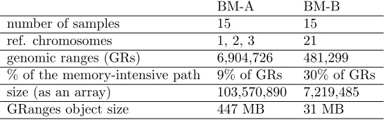
For simplicity, the two benchmarks are named BM-A and BM-B. Table 3 presents the
relevant details about both benchmarks. Specifically, BM-B is used to measure host memory
BM-A BM-B
number of samples 15 15
ref. chromosomes 1, 2, 3 21
genomic ranges (GRs) 6,904,726 481,299
% of the memory-intensive path 9% of GRs 30% of GRs
size (as an array) 103,570,890 7,219,485
GRanges object size 447 MB 31 MB
Table 3: Technical details of used benchmarks
footprints and to conduct sensitivity analysis. Meanwhile, BM-A is used to evaluate both gcn.MOPS and cn.MOPS since its size is sufficiently larger than BM-B.
6
Results
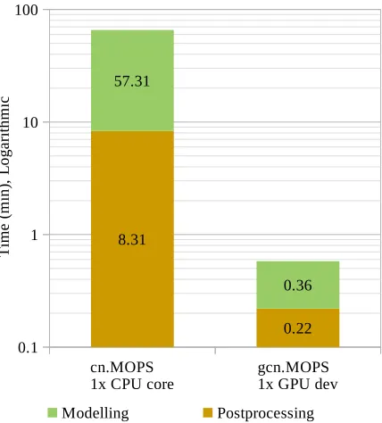
Figure5presents the execution time, on logarithmic scale, of both gcn.MOPS and cn.MOPS in the modelling and postprocessing steps for BM-A. In the modelling step, gcn.MOPS achieved
a speedup of 159.19× relative to cn.MOPS. This speedup is substantially higher than the
projected maximum achievable speedup with multi-CPU parallelism ψCP Umax
. In Section2, it was shown thatψCP U
max .9.24×. In the postprocessing step, gcn.MOPS decreased the execution
time by 97% relative to cn.MOPS. This ratio is expected to remain fairly constant for larger problems. The reason is that in gcn.MOPS, this stage is mostly limited to assigning names to rows and columns of various matrices, which can be regarded as a relatively trivial operation.
In both steps combined, gcn.MOPS has a lower host memory footprint running BM-B relative to cn.MOPS. The peak memory usage of the gcn.MOPS is 711.2 MB vs 1,726.5 MB for cn.MOPS. In other words, we reduce memory usage by 58% or almost 1 GB in BM-B. This reduction in host memory usage is expected since results are not duplicated in the postprocessing step to change data organization as required by cn.MOPS.
7
Conclusion
In short, the modelling step of cn.MOPS, a CNV detection tool, is alternatively accelerated
with GPU. The new solution, gcn.MOPS, achieved a speedup factor of 159×in the modelling
step. Such a speedup factor is considerably higher than the maximum of what can be achieved
with cn.MOPS, which is found to be.9.24×. Moreover, the execution time of the
cn.MOPS
1x CPU core gcn.MOPS1x GPU dev 0.1
1 10 100
8.31
0.22 57.31
0.36
Modelling Postprocessing
T
im
e
(m
in
),
L
og
ar
ith
m
ic
Figure 5: gcn.MOPS vs cn.MOPS: execution time in the modelling and the postprocessing steps for benchmark BM-A
These performance levels are achieved by applying various optimization techniques to make the core algorithm fit the GPU architecture. Data access patterns are changed to ensure coa-lesced memory accesses. This results in an efficient use of GPU memory and an almost-complete elimination of the data postprocessing steps. Additionally, branch divergence is made minimal by decoupling the non-compute path from the compute-intensive path of the algorithm. The former is executed on CPU and the associated execution time is hidden by host/device con-currency. Other applied optimization techniques include using constant memory and disabling L1 cache memory. Potentially, more performance might be gained with for-loop unrolling, but this can impact software complexity and readability.
For the setup used, the modelling and the data postprocessing steps in gcn.MOPS
ac-count for ∼1.3% of the pipeline’s total execution time as opposed to ∼58.7% in cn.MOPS
using 1× CPU core. Thus, other pipeline stages should be investigated for GPU execution.
Meanwhile, further improvements to gcn.MOPS should be limited to ensuring cross-device and cross-platform compatibility.
8
Acknowledgments
References
[1] T. M. Davies. The Book of R: A First Course in Programming and Statistics. William Pollock, San Francisco, CA, 2016.
[2] Guenter Klambauer, Karin Schwarzbauer, Andreas Mayr, Andreas Mitterecker, Djork-Arne Clevert, Ulrich Bodenhofer, and Sepp Hochreiter. cn.mops: Mixture of poissons for discovering copy number variations in next generation sequencing data with a low false discovery rate.Nucleic Acids Research, 40:e69, 2012.
[3] Wetterstrand KS. The cost of sequencing a human genome.
https://www.genome.gov/sequencingcosts, July 2016. Accessed: 10 Feb 2017. [4] nVidia. Profiler user’s guide.
http://docs.nvidia.com/cuda/profiler-users-guide. Accessed: 30 Mar 2017. [5] U.S. National Library of Medicine. Congressional justification FY 2015.
https://www.nlm.nih.gov/about/2015CJ.html, Feb 2015. Accessed: 10 Feb 2017.
[6] Renjie Tan, Yadong Wang, Sarah E. Kleinstein, Yongzhuang Liu, Xiaolin Zhu, Hongzhe Guo, Qinghua Jiang, Andrew S. Allen, and Mingfu Zhu. An evaluation of copy number variation detection tools from whole-exome sequencing data. Human Mutation, 35(7):899–907, 2014.
A
Benchmarking Samples
The following is the list of samples used to construct performance benchmarks:
1. NA07048.mapped.ILLUMINA.bwa.CEU.exome.20120522.bam 2. NA07051.mapped.ILLUMINA.bwa.CEU.exome.20120522.bam 3. NA06984.mapped.ILLUMINA.bwa.CEU.exome.20120522.bam
4. NA06986.mapped.ILLUMINA.bwa.CEU.exome.20121211.bam 5. NA06989.mapped.ILLUMINA.bwa.CEU.exome.20120522.bam 6. NA07037.mapped.ILLUMINA.bwa.CEU.exome.20121211.bam 7. NA11933.mapped.ILLUMINA.bwa.CEU.exome.20121211.bam 8. NA07347.mapped.ILLUMINA.bwa.CEU.exome.20121211.bam 9. NA10847.mapped.ILLUMINA.bwa.CEU.exome.20121211.bam