Volume 39 - Article 4 | Pages 95–135

(1)

VOLUME 39, ARTICLE 4, PAGES 95

,

135 PUBLISHED 17 JULY 2018

http://www.demographic-research.org/Volumes/Vol39/4/ DOI: 10.4054/DemRes.2018.39.4

Research Article

Leaving home in 19th century England and

Wales: A spatial analysis

Joseph Day

This publication is part of the Special Collection on “Spatial analysis in historical demography: Micro and macro approaches,” organized by Guest Editors Martin Dribe, Diego Ramiro Fariñas, and Don Lafreniere.

T This open-access work is published under the terms of the Creative Commons Attribution 3.0 Germany (CC BY 3.0 DE), which permits use, reproduction, and distribution in any medium, provided the original author(s) and source are given credit.

(2)

1 Introduction 96

2 Data and methods 97

2.1 Using the 1881 census of England and Wales 97

2.2 Measuring the age at leaving home 98

3 Age at leaving home 103

4 Life-cycle service and leaving home 108

5 Household determinants of leaving home 115

6 Modelling the determinants of leaving home 119

7 Conclusion 124

References 126

(3)

Leaving home in 19

th

century England and Wales:

A spatial analysis

Joseph Day1

Abstract

BACKGROUND

The process and timing of leaving home represents a major demographic transition which has an impact on other demographic events such as migration and marriage.

OBJECTIVE

This paper aims to accurately measure the leaving home process across England and Wales in 1881 at a high spatial resolution and to analyse the determinants of regional disparities in the leaving home process. The paper is designed to shift the focus away from the household- and individual-level determinants of leaving home and to the relationship with the socioeconomic context.

METHODS

This paper uses data from the complete individual-level returns from the 1881 census of England and Wales. Using standard demographic techniques to adjust for parental mortality, a spatial framework is used to analyse the relationship between the leaving home process and the socioeconomic context. Moran’s global and local i is used to identify spatially-determined variables such that their effect on the age at leaving home can be evaluated in an OLS model.

RESULTS

The leaving home process exhibits a clear spatial pattern related to the institution of service. Poor households responded to hardship by either retaining or ejecting children from the home depending on the prevalence of service.

CONTRIBUTION

This article adds to the literature on the leaving home process by mapping variations in the mean age at leaving home across England and Wales in 1881 rather than relying on small region-specific samples. Through the comprehensive use of the census, this process can be linked to the socioeconomic context, thereby explicating households’ varying responses to poverty in 19th_{century England and Wales.}

(4)

1. Introduction

The process of leaving the parental home is an important but understudied phenomenon that can tell us much about the structure of societies, both past and present. Although Pooley and Turnbull are keen to stress that in the past leaving home was seldom a ‘once and for all’ move, with many individuals returning to the parental home at least once in their lifetime, the act of leaving was a fairly universal phenomenon, with over 90% of men and women doing so at some point in their lives (Pooley and Turnbull 1997; Pooley and Turnbull 1998; Pooley and Turnbull 2004; Schürer 2004). Consequently, leaving home is a significant lifecycle transition in both historic and contemporary populations.

Most studies of the leaving home process employ longitudinal datasets to study the leaving home process and analyse the role that socioeconomic context and household and individual characteristics had on the age of exit from the parental home (Bras and Kok 2004). For example, Guinnane finds that males left home later than females in rural Ireland, reflecting an inheritance system that led many sons to never leave home (Guinnane 1992). Conversely, Bras and Kok compare rural Zeeland with urban Utrecht in the Netherlands and find that urban males were more likely to leave home than rural girls, and that household characteristics such as the number of younger siblings present in the household had the largest effect determining the likelihood of leaving home (Bras and Kok 2004).

However, although such studies explicitly incorporate individual, household, and socioeconomic characteristics into models of the age at leaving home, the longitudinal datasets employed to analyse the process are generally drawn from small regional samples. In a fixed effect model a uniquely ‘urban’ or ‘rural’ effect can only be convincingly distinguished from other predictors if the model is fully specified and exhibits no significant multicollinearity with any other predictors (Field 2009). Where data is drawn from a small sample – one urban and one rural settlement, for example – the extent to which the age at leaving home is the product of either a uniquely urban effect or a missing variable which the urban dummy variable is collinear with cannot be inferred in a fixed effect model.

(5)

do not exhibit any multicollinearity such as might be present in smaller samples, meaning that the effect which different socioeconomic contexts had on the leaving home process can be derived with more confidence. To accomplish this, this paper will explore the relationship between socioeconomic context and the leaving home process in three sections: the regional distribution of the age at leaving home, its relationship to the institution of service, and a formal analysis of the relationship between the institution of service, the household economy, and the moment of exit from the home.

2. Data and methods

2.1 Using the 1881 census of England and Wales

(6)

chosen because they were more spatially refined than the 632 registration districts (RDs) but were still large enough to avoid small number problems.2

Performing a spatial analysis by mapping the variation in the leaving home process across England and Wales and analysing its relationship to the socioeconomic context has two main advantages. First, it is the most efficacious means of presenting the data in 2,192 SRDs, and second, it allows for a model of the leaving home process that is fully specified. Whereas non-spatial modelling assumes that events are independent, a spatial model acknowledges spatial dependency: “everything is related to everything else, but near things are more related than distant things” (Tobler 1970). Therefore, whereas a non-spatial plot of the residuals might indicate that they are randomly distributed, a spatial analysis might suggest that the residuals are clustered in space. Spatially clustered residuals might provide evidence of explanatory variables which a nonspatial analysis might miss.

Consequently, as this paper analyses the relationship between leaving the parental home and the socioeconomic context in which it occurs, it is necessary to estimate from where individuals’ left home. Using the census, individuals’ stated parish of birth is assumed to also be the parish in which their parental home was located. The next section outlines the methodology adopted to measure the leaving home process from census evidence.

2.2 Measuring the age at leaving home

First, this paper assumes that if children were not living with their parents on census night it was the result of a conscious decision by either parents or child. In other words, children either chose to leave or their parents forced them to do so. In reality, however, children may not have been resident with their parents on census night for many other reasons: they may have been temporarily resident with relatives or permanently living with guardians other than their parents, and would therefore still consider themselves to be living at ‘home’, in spite of it not being their natal home (Hareven and Adams 2004). Although it is not possible to account for the multiplicity of individual definitions of ‘home’, it is possible to account for another major reason why children may not have been resident with at least one parent on census night: the death of both parents.

To estimate the number of orphans, regional measures of parental mortality were made by first estimating the mean age of mothers at the birth of their coresident children in each sub-registration district (SRD). This is shown in Figure 1. Figure 2

2_{In 1881, 2,175 sub-registration districts (SRDs) were nested in 630 registration districts (RDs), which were}

(7)

estimates the mean age of fathers by adjusting mothers’ mean age by the average age gap between husbands and wives. Age-specific mortality rates ( ) in each registration district (RD) were calculated and form the basis for the estimates of parental mortality.3

Figure 1: Mean age of mother at birth of her child, Sub-Registration District (SRD) of residence, England and Wales, 1881

Source: Schürer and Woollard (2003).1881 Census of Great Britain [computer file]. UK Data Archive [distributor].

3_{Mortality rates} _{and survival probabilities} _{are standard life table measures and do not need further}

explanation here. The calculation of life tables is fully documented in: Newell, C. (1988). Methods and

models in demography. Chichester: Wiley: 67–71. A worked example of the age-specific likelihood of being orphaned by the age of 30 is shown in the Appendix Table A-1. As the units – registration districts (RDs) – in which mortality data was reported changed in the period 1851–1881, these units were interpolated onto a standardised geography so that mortality rates could be mapped over time and the cumulative likelihood of being orphaned at any time between 1851 and 1881 could be accurately calculated. See: Southall, H.R.,

Gilbert, D.R. and Gregory, I.N. (1998)Great Britain Historical Database: Census Statistics, Demography,

(8)

Figure 2: Mean age of father at birth of his child, Sub-Registration District (SRD) of residence, England and Wales, 1881

Source: Schürer and Woollard (2003). 1881 Census of Great Britain [computer file]. UK Data Archive [distributor].

Table A-1 in the Appendix shows the likelihood that an individual born in Berwick-upon-Tweed and aged 30 in 1881 had been orphaned by the time of the 1881 census. It assumes that parents were at the mean age of childbearing for their SRD as shown in Figures 1 and 2. The cumulative likelihood that the mother and father had survived each year between 1851 and 1881 was 67.8% and 60.4% respectively, making the likelihood that they had died at any point up to it 32.2% and 39.6%. The likelihood that they had both died is the product of this: 12.7%. Although this is an imperfect estimate of parental mortality as it is assumes that the mortality risks of spouses are unrelated despite evidence to the contrary, no better data exists for 19th_{century England}

(9)

Figure 3: Likelihood that individuals aged 21 have lost both parents, England and Wales, 1881

Source:Schürer and Woollard (2003). 1881 Census of Great Britain [computer file]. UK Data Archive [distributor]; Southall, Gilbert, and Gregory (1998). Great Britain Historical Database: Census Statistics, Demography, 1841–1931 [computer file]. UK Data Archive [distributor].

Figure 4: Percentage of coresident children born over 10 km away and in a different SRD to their SRD of residence, England and Wales, 1881

(10)

Consequently, in order to measure the age at leaving home it is necessary to proxy the parish in which the parental home was located. This is straightforward where individuals were still coresident with their parents, but where individuals were no longer coresident with their parents the parish in which their parental home was located had to be estimated. In practice, this meant determining whether individuals’ place of birth or place of residence was the best proxy for the parish from which they left home. However, it is implausible to assume that individuals’ parental home was always located in their parish of current residence, and that individuals never migrated independently of their family. It is equally implausible to assume that the parental home was always located in their parish of birth, and that family migration never took place.

Therefore, the likely location of an individual’s parental home was weighted between their place of birth and place of residence as recorded in the 1881 census. Although Ravenstein argues that single adults were the most migratory group, White and Schürer find that family groups migrated more than Ravenstein supposes (Ravenstein 1885; Ravenstein 1889; Lawton 1968). In his comparative study of family migration in Scunthorpe and Grantham in 1881, White estimates that around a third of the population entered Grantham with family, compared to over two-thirds of migrants to Scunthorpe (White 1988). Schürer similarly finds that family migrants consisted of around 30% of the total in rural Essex between 1861 and 1881 (Schürer 1989). As family migration had an effect on where individuals’ parental home was estimated to be, it must be accounted for.

The proportion of individuals still coresident with their parents but resident in a different SRD to the one in which they were born was calculated. The regional estimates for this are shown in Figure 4. In Berwick-upon-Tweed, for example, 13.4% of coresident children were born elsewhere. It was therefore inferred that 13.4% of the population that did not live with their parents had already migrated to Berwick-upon-Tweed with their family. Individuals’ parental home was therefore weighted 0.134 to Berwick-upon-Tweed and 0.866 to their parish of birth.4_{Although this is not a perfect}

assumption, as individuals may have left home from an intermediate parish, it is better than the alternative assumption that an individual’s parental home was located in either their parish of birth or their parish of residence. Having made adjustments for both parental mortality and family migration, Table A-2 in the Appendix shows how these adjustments produced an estimate of the population that had/had not left home.

Having made these adjustments, the mean age at leaving home was calculated using a variation of Hajnal’s calculation of the singulate mean age at marriage

4_{Although the likelihood of migrating with/without family varied by age cohort, this was not accounted for so}

(11)

(SMAM)5_{– the singulate mean age at leaving home (SMAL) (Steckel 1996; Schürer}

2004). Essentially, the SMAL calculates an estimate of the mean age at leaving home from the age-specific proportion of the population that were/were not at home. Unlike the SMAM, which measures the mean age at first marriage from the age-specific proportion of the population that were ever married, census evidence does not identify those that had ever left home, only those that either were or were not coresident with their parents on census night. Therefore, although the SMAL is not a measure of those who had ever left home, in the way the SMAM is a measure of those that had ever married, this is not necessarily a disadvantage of the data. In their analysis of longitudinal data from family histories, Pooley and Turnbull identify numerous examples of children returning to the parental home, noting that leaving home was rarely a once-and-for-all move in the way that marriage was (Pooley and Turnbull 1997). As individuals often returned home, estimating the mean age at which children first left home would be misleading.

Using the complete CEBs, the SMAL can be measured, mapped, and analysed across England and Wales, and once the adjustments outlined above are made the SMAL captures the average leaving home experience, rather than simply the first move. Table A-3 in the Appendix outlines its calculation. Thus, the population that had not left home was estimated and the SMAL was calculated. By removing the confounding effect of parental mortality this aims to measure the age of leaving home as a consequence of individual choice and agency, rather than the age at which coresidence ceases.

3. Age at leaving home

Although the SMAL is a useful measure of the leaving home process and can be used to analyse both the spatial variation in the age at leaving home and in modelling its socioeconomic determinants, the SMAL only represents the mean experience. In order to build a more complete picture of leaving home it is necessary to explore its variance of experience at both the national and the regional level.

5_{The SMAM is a measure of the age at marriage derived by Hajnal for use on age-specific marital status data}

commonly available in population censuses. It is a substitute for the true mean age, which can be calculated directly from the ages given on marriage certificates or in family reconstitution studies where age at marriage may be determined by linking entries in baptism and marriage registers. See: Hajnal, J. (1953). Age at

marriage and proportions marrying. Population Studies 7:111–136; Hajnal, J. (1965). European marriage

patterns in perspective. In: Glass, D.V. and Eversley, D.E.C. (eds.).Population in history: Essays in historical

demography.London: Routledge: 101–143; Schürer, K. (1989). A note concerning the calculation of the

singulate mean age at marriage.Local Population Studies 43: 67–70; Woods, R.I. (2000).Demography of

(12)

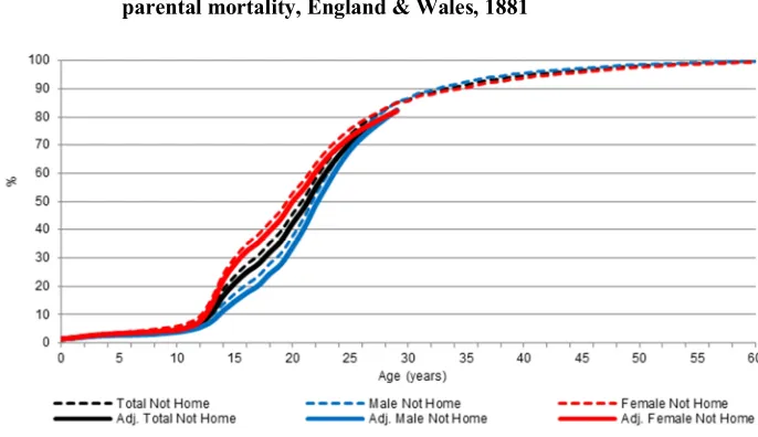
Figure 5: Proportion of age-specific population no longer at home, adjusted for parental mortality, England & Wales, 1881

(13)

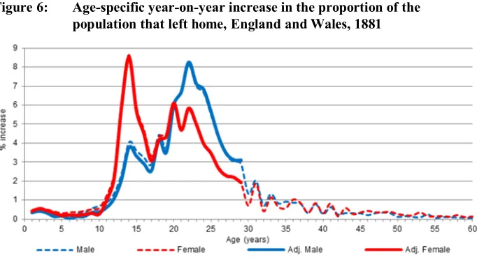
Figure 6: Age-specific year-on-year increase in the proportion of the population that left home, England and Wales, 1881

Here it is evident that while the speed of female exit from the parental home peaked around the age of 14 and then again around the age of 21, in the male case the pattern was reversed. Here, there was a significant minority leaving home around 14, while the majority did so at 21. Thus, although superficially the male and female experiences do not appear to have had much in common, both display spikes of ‘early’ and ‘late’ leavers. Therefore, rather than analysing the leaving home process by gender, a more meaningful distinction might be between those that left home ‘early’ and those that left ‘late’.

(14)

Figure 7: Smoothed male singulate mean age at leaving home (SMAL), England and Wales, 18816

Figure 8: Agricultural and industrial settlement types, male occupations, England and Wales, 1881

6_{Rates were first smoothed using an empirical Bayes rate standardisation. The resultant SMAL was then}

mapped and spatially smoothed using a real interpolation.

SMAL < 12 years old 12 - 15 years old 16 years old 17 years old 18 years old 19 years old 20 years old 21 years old 22 years old 23 - 24 years old > 24 years old

(15)

Although Pooley and Turnbull (1997) estimate the male and female mean age at leaving home to have been 23.9 and 23.4 years respectively between 1850 and 1889, as opposed to the 22.2 and 20.6 years estimated here, this is likely a consequence of the nonrepresentative sample they used. Whereas the SMALs reported here use the complete CEBs from England and Wales, Pooley and Turnbull use a sample of 16,091 family histories that are not necessarily nationally representative, highlighting a flaw in the methodology adopted by that study (Pooley and Turnbull 1998). Only their estimates of the mean age at which the sons/daughters of agricultural labourers left home approach the estimates given here. In that case they estimate sons and daughters to have left home at 23.2 and 20.9 years on average, respectively (Pooley and Turnbull 1997).

Having mapped the SMAL, it is evident that the leaving home process was strongly affected by the three economic regimes shown in Figure 8. The industrialised mining and manufacturing districts are shown in red, family farming in green, and capitalist agriculture in grey.7_{Even a cursory comparison of the geography of leaving}

home with the occupational structure of 19th_{century England and Wales suggests a}

strong correlation. Indeed, even a simple OLS correlation of the male SMAL and the propensity to enter farm service produces an R of 0.57 and a coefficient of –0.06, indicating that a 1% increase in the proportion of the population entering farm service upon leaving home reduced the SMAL by around 23 days.

It is by no means a novel observation that the institution of service was a determinant of leaving home. Schürer argues that the rise in the age at leaving home and the slowing rate of exit from the parental home over the 19th_{and early 20}th

centuries appears to have gone hand in hand with the decline in farm service and the rise of urbanisation and industrialisation (Schürer 2004). Mitterauer likewise notes that service was replaced by “living at home but working outside it [and]...leaving home came to be connected increasingly with marriage and the upper threshold of youth” (Mitteraurer 1992).,Although the institution of service was the most significant determinant of the leaving home process, its effect has until now been explained in terms of the demand for labour, rather than its supply. This, however, does not explain the incentives that individuals had to enter service. Did individuals leave the parental home to enter farm service because they perceived that doing so would be in their own best interest, or did they leave as the result of parental pressure? This is the focus of the next section.

7_{Industrial regions were defined as such if more than half the occupied male population were employed in the}

(16)

4. Life-cycle service and leaving home

Kussmaul’s landmark and comprehensive account of service in husbandry in early modern England establishes the orthodoxy that from the late 18th century onwards in the south east of England the combination of a growing population, a rising poor relief bill, and a decline in real wages led capitalist farmers to reject farm service in favour of a more casual proletarianised labour force (Kussmaul 2008; Gritt 2002; Snell 1985). By contrast, in the north and west of England farm service remained an important means of labour procurement, which both Gritt and Howkins interpret as a flexible response to the increasing tension between the labour demands of agriculture and industry (Howkins and Verdon 2008; Gritt 2000). Goose is equally unequivocal as to the geography of farm service in the 19th_{century: “...farm servants survived in much}

greater numbers for far longer in the north and south-west of England, where pasture farming predominated, settlements were more dispersed, farms were generally smaller and alternative employment in rural industries more readily available. In the southern half of the country, however, excluding only Cornwall and Devon, farm service was in general decline” (Goose 2006).

(17)

Figure 9: Smoothed male singulate mean age at leaving home (SMAL), simplified visualisation, England and Wales, 1881

Making the same point from a different angle, both Katz and Kett find that the leaving home process was often slower and more responsive to shifting economic conditions in the 19th_{century (Katz 1975; Kett 1977). The implication is that a slow}

rate of exit from the parental home reflected economic pragmatism while a fast rate reflected institutionalised socioeconomic norms (Hareven and Adams 2004). Figures 10 and 11 therefore analyse where the leaving home process was ‘low’, ‘medium’, and ‘high’ in order to determine if there was a relationship between the mean age at leaving home and the rapidity with which the process occurred. For example, did the leaving home process occur very quickly where the SMAL was low, suggesting a low age of leaving home was a response to an institutionalised cultural norm?

The age of leaving home was defined as low, medium, or high by analysing the pseudo F-statistic. This was highest – reflecting maximal within-group similarity and between-group difference – when the SMALs were grouped into three categories: a low age at leaving home of under 19 years old, a medium age at leaving home of between 19 and 22, and a high age at leaving home of 22 years or more. These three groups are mapped in Figure 9. Not only is the correlation between high, medium, and low SMALs with industrial, capitalist farming and family farming districts even more apparent, but analysing the leaving home process in these three regions in Figures 10 and 11 suggests

(18)

a relationship between the average age of leaving home and the speed at which the process occurred.

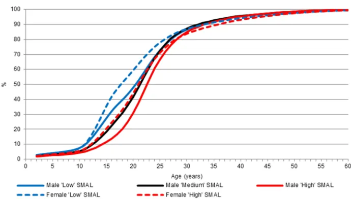
Analysing the interquartile range – the ages between which the central 50% of the population left the parental home – in Figure 10, it appears that the leaving home process became longer and more drawn out as the mean age of leaving home decreased. This shows that in the male ‘low’ SMAL SRDs, concentrated mainly in the family-farm-dominated agricultural north and west, half of the population exited the parental home between the ages of 14 and 25, a process taking 11 years. In the ‘medium’ SMAL zones found predominantly in the south east of England the central 50% left home in just 9 years between the ages of 16.5 and 25.5, while in the ‘high’ SMAL industrial towns and cities it took just 8 years, occurring between the ages of 19 and 27. For females, on the other hand, the process was completed in just 10 years in both the ‘high’ and ‘low’ SMAL zones, the only difference being that in ‘low’ SMAL rural England and Wales it occurred between the ages of 14 and 24 compared to 16 and 26 in the ‘high’ SMAL urban-industrial centres of England and Wales. This shows that late leavers had the highest rates of exit, contrary to analyses which show that a rapid pace of exit was associated with a low age of leaving home.

Figure 10: Proportion of age-specific population no longer at home, by SMAL type, England and Wales, 1881

(19)

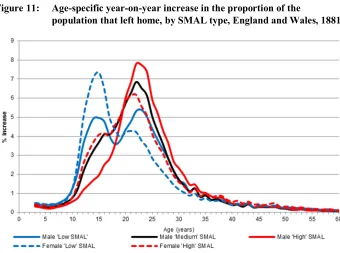
Although Figure 11 also shows that in the ‘high’ SMAL regions of England and Wales the process began late, peaked around the age of 22, and then began to slow until it was complete by around the age of 30, the process in the ‘low’ SMAL regions is more mixed, especially the male experience. Here, there are two distinct peaks in the leaving home process at 15 and 23, and while the leaving home process in the ‘high’ SMAL urban-industrial districts had barely started by the time sons were 15 – just 10% having done so – 1-in-3 15-year-old boys had left home in the ‘low’ SMAL rural north and west. Yet even though the process of leaving home had begun far earlier in the ‘low’ SMAL zones, it did not finish any earlier than elsewhere.

Figure 11: Age-specific year-on-year increase in the proportion of the

population that left home, by SMAL type, England and Wales, 1881

(20)

SMAL rural England, while just 14% of 16-year-old males had left home in the ‘high’ SMAL districts. Clearly, for a substantial minority there were strong incentives for coresidence to end both early and rapidly.

According to the literature, a rapid rate of exit from the parental home suggests that the process is being driven by cultural and institutional norms. It therefore seems plausible that this might also have been a significant determinant for the rapid exit of both sons and daughters in the ‘low’ SMAL zones of England and Wales. If this is correct, a strong correlation would be expected between the SMAL and the age at which the population were perceived as having become adult. This can be tested using the 1881 CEBs. Occupational descriptors often include gendered job titles such as ‘errand boy’, ‘shop girl’, ‘postman’, and ‘washerwoman’, which, when combined with an individual’s age, can be used to ascertain the ages at which individuals defined themselves as having transitioned from childhood to adulthood.8

Figure 12 contrasts the age-specific proportion of females describing themselves as a “woman” as opposed to a “girl” with the age-specific proportion of females that had left the parental home. From this, not only is it clear that the female leaving-home profile varied significantly between regions, but also that in agricultural England, half the females had become “women” by the age of 15.9; almost precisely the same age at which half of agricultural-born females had exited the parental home. By contrast, in the mining communities females appear to have been defined as adult much later than the national average of 16.8, which suggests that female adulthood was defined more in terms of functionality. Indeed, in agricultural districts, females tended to exit the home relatively early – around the age of 16 or 17 – usually to enter domestic service, while daughters in manufacturing England tended to be employed in the textile mills while still resident with their parents. Females in agricultural and manufacturing England and Wales were therefore more functionally ‘adult’ than their counterparts in mining towns, who tended to remain out of the formal labour force, were chiefly occupied in assisting their mothers with domestic work, and only exited the parental home upon marriage (Shaw-Taylor 2007). Thus, adulthood came later to those daughters who remained subordinate to their mothers for longer and who entered the adult sphere through marriage rather than through gainful employment in either the factory or domestic service (Goldscheider and Goldscheider 1989).

8_{Only records with the terms ‘boy’, ‘girl’, ‘man’, or ‘woman’ in their occupation descriptor were included.}

(21)

Figure 12: Percentage of females describing themselves as girl/woman vs. percentage of females that left home in key parish types, England and Wales, 1881

(22)

Figure 13: Percentage of males describing themselves as boy/man vs. percentage of males that left home, England and Wales, 1881

(23)

5. Household determinants of leaving home

As a cross-sectional source, it is not possible to use the census to identify the households that ejected children. Instead, households’ incentives to remove children can be inferred from the incentives of households to retain them. Using indirect age-standardisation in Figure 14, a participation index was produced whereby the number of occupied sons was compared with the number that might be expected given their age distribution, and the age-specific male participation rate in each SRD. This shows that those sons resident with fathers in farm service districts (highlighted in crosshatchings) were significantly less likely to be employed compared to all males in their SRD.

Figure 14: Age-standardised participation rate of males coresident with parents, England and Wales, 1881

For example, sons in Brecknockshire that were still coresident with at least one parent were about half as likely to be employed compared to the average participation rate in Brecknockshire. By contrast, in the rest of England and Wales coresident sons were no more or less likely to be occupied than the population at large. Therefore, in the farm service districts (indicated in Figures 14 and 15 by cross-hatchings) there appears to have been significantly less opportunity for employment that sons could undertake while still at home. This partly explains why so many entered farm service, as it must have been the only means of employment for sons. Testing for the statistical significance of this by running Moran’s local in Figure 15 clarifies this point (Moran

Age-standardise d participation rate

(24)

1950). Moran’s local is a standard statistical test of spatial association used to evaluate the extent to which a variable is spatially clustered. Whereas Moran’s global measures overall clustering of the data, Moran’s local identifies local clusters. This statistic therefore picks up local clusters of high and low values, which the global measure does not (Anselin 1995). This confirms that the participation rate among sons still living with their parents was significantly lower in the service zones of England and Wales.9

However, Figure 11 has shown that even in the ‘low’ SMAL regions the leaving home process was split between those that left home upon reaching adulthood and those that left later. Therefore, were the sons of certain groups more likely to be unemployed compared to others, and did this affect the moment of exit from the parental home?10

Figure 15: Cluster type of age-standardised participation rate of males coresident with parents, England and Wales, 1881

9_{As space precludes an analysis of both sons and daughters, this section focuses on the male experience of}

leaving home and entering farm service at the expense of the female experience of domestic service. This decision is justified on the basis that the characteristics of households that retained daughters compared to those that did not were virtually identical to the characteristics of households that retained/removed sons. The relationship between households that did/did not retain children and the institution of service is also far clearer visually in the context of farm service than of domestic service, given its clear geography compared to the industrialised towns and cities and the agricultural south-east. The characteristics of households that retained/ejected sons and the conclusions drawn are also applicable to households that retained/ejected daughters.

10_{Individuals are considered ‘employed’ if they receive payment in kind outside of the home or a cash wage.}

Family members working as servants in their own home are not considered to be employed in this analysis.

(25)

Figure 16 maps the age-standardised unemployment rate of sons whose fathers’ HiS-CAM score was above 52 as a proportion of the unemployment rate amongst sons whose fathers’ HiS-CAM score was 52 or below. HiS-CAM, rather than HiS-CLASS, is used to analyse variation between socioeconomic classes because HiS-CAM has two main advantages over HiS-CLASS (Armstrong 1972; Armstrong 1974; Mills and Drake 1994; Higgs 2005; Stewart, Prandy, and Blackburn 1973; Stewart, Prandy, and Blackburn 1980; Prandy and Lambert 2003). Whereas HiS-CLASS imposes a structure based on the occupations that are presumed to be professional, skilled, unskilled etc. and divides occupations into twelve classes, HiS-CAM allows structures and classifications to emerge from the data, allowing for analysis on a continuous socioeconomic scale (Lambert et al. 2013). Briefly, HiS-CAM is a historical version of the CAMSIS approach to determining the relative stratification position of incumbents of various occupations based on their level of interaction with individuals in other occupations. The CAMSIS measures are constructed using data on pairs of occupations linked by a social interaction such as marriage, friendship, or parent-child relationship. By asking, for example, how many friends of bakers are bakers/butchers etc., the relative social distance between these occupations is established (Lambert et al. 2013). The scale was then standardised between 0 and 100, making 50 the median HiS-CAM score (Prandy and Bottero 2000). Several scales were produced, generated from the given occupations of bridegrooms’ and brides’ fathers listed in marriage registers. The most appropriate for England and Wales in 1881 is version 1.3.1.E, which was produced based on intergenerational occupational pairs from seven countries between 1800 and 1890 (Lambert et al. 2013).

(26)

Figure 16: Smoothed age-adjusted unemployment rate of sons where fathers’ HIS-CAM score were over/under 52, England and Wales, 1881

Source:Schürer and Woollard (2003). 1881 Census of Great Britain [computer file]. UK Data Archive [distributor].

Figure 17: Cluster type of male ‘at home’ unemployment rate where fathers’ HIS-CAM scores were over/under 52, England and Wales, 1881

Source:Schürer and Woollard (2003). 1881 Census of Great Britain [computer file]. UK Data Archive [distributor].

Unemploym ent rate < 0.81 0.81 - 0.85 0.85 - 0.89 0.89 - 0.93 0.93 - 0.97 0.97 - 1.03 1.03 - 1.05 1.05 - 1.07 1.07 - 1.09 1.09 - 1.11 > 1.11

(27)

Therefore, the presence of farm service implied an absence of alternative occupations for the sons of the poor and unskilled, consequently funnelling them into farm service and guaranteeing a supply of agricultural labour. Where this institution was absent, however, the sons of the poor had access to employment that did not require them to leave the parental home. Poor unskilled households responded to the presence of farm service by putting children into service as soon as they reached the perceived age of adulthood. This did not occur where farm service was not present, as poor households largely sought to retain children as potential wage earners. This was not an option in the farm-service-dominated agricultural north and west, where the coresident sons of the poor and unskilled were significantly less likely to find employment. Evidently, children from the agricultural north and west had no option but to leave home in order to find employment.

It is worth noting that these conclusions could only be drawn from a spatial analysis. A visual inspection clearly shows that the spatial structure of the leaving home process was a function of the socioeconomic regime in which the process occurred, and determining the relationship between the leaving home process, the socioeconomic context, and the household could only be achieved spatially. Here, again, it was demonstrated that there was a strong spatial correlation between family farming regions, low SMALs, and the likelihood that the sons of poorer fathers were unemployed, suggesting that sons of poor fathers were incentivised to stay at home in the agricultural south-east to bring in a wage, but left in the agricultural north and west to enter service, given a paucity of alternatives. This could only be observed spatially and demonstrates the value of spatial analysis as an exploratory tool. Having identified these variables, the next section incorporates these predictors into a more formal model of the SMAL.

6. Modelling the determinants of leaving home

This article has sought to measure the leaving home process and to relate the mean age at leaving to the socioeconomic context, specifically the institution of service. However, this is by no means the complete story. The evidence presented here has only shown that the institution of service resulted in early exit from the parental home for the children of the unskilled, given a lack of alternative sources of employment. While this illustrates how and why service was a determinant of leaving home, it does not show whether children left home as a result of parental pressure or because they perceived it to be in their own best interest.

(28)

This can be best illustrated by showing that the institution of service alone does not sufficiently account for the regional variation in the age at leaving home. Figure 18 shows the male SMAL model from the prevalence of the institution of service, as predicted in a global OLS.11_{Although service accounts for 0.57 of total variance, and}

plotting the predicted SMAL against the standardised residual – as well as other standard diagnostic and validation tests – indicates that the error is stochastic, Figure 19 analyses the spatial clustering of the residuals using Moran’s local . It shows that the observed SMAL was significantly lower in the south east of England than is predicted by the prevalence of service, and higher in the industrial districts. Clearly, variables are missing which better capture the spatial variation in the SMAL. An OLS regression was therefore run to identify these missing variables.

Figure 18: Estimated male SMAL from OLS model with proportion of males in service after exiting the parental home as the predictor, England and Wales, 1881

Table 1 shows three models that contribute towards building a fully specified model of the male SMAL. Model 1 shows the effect of service alone, while model 2 includes all relevant variables that describe the characteristics of individuals’ place of origin. However, the timing of individuals’ exit from the parental home was governed not just by ‘push’ factors present at an individual’s registration district (RD) of origin,

11_{As before, the prevalence of service is estimated by the proportion of the male population described as}

servants in the 1881 census when aged within two years of the calculated SMAL in their SRD of origin.

(29)

but also by the attractiveness of their chosen destination relative to their origin (White and Woods 1980). Therefore, model 3 also includes variables that describe the characteristics of individuals’ chosen destination, as well as variables describing the differences between migrants’ origin and destination.

Table 1: OLS regression of male singulate mean age at leaving home (SMAL)

Model 1 Model 2 Model 3

Coefficient Coefficient Coefficient

Dependent Variable:Male SMAL

Constant 21.953 17.522 21.56

% of males in service (place of birth) –0.06 –0.06 –0.05

Participation rate (place of birth) 0.11 0.09

% of males in manufacturing/mining (place of birth) 1.13 1.09

Father’s HiS-CAM score 14.52 8.72

Distance migrated (km) –0.70

HiS-CAM score change (Place of residence –

place of birth) –8.35

Population density change (Place of residence –

place of birth) 0.09

R2 0.57 0.64 0.71

Adj. R2 _0.57 _0.64 _0.71

N 2,192 2,192 2,192

Notes: All regressions are OLS. All variables are significant at the <0.01 confidence level.

(30)

influential cases and none were found to be significant. All VIF values were between 1.2 and 3.6, significantly less than the score of 7.5 that would indicate multicollinearity and redundant variables. All p-values were less than 0.01 Having validated the models, it appears that each subsequent model explains more variance than the previous one, as missing variables describing migrants’ origin were included in model 2, and variables describing migrants’ destination were included in model 3, first raising the to 0.64 in model 2 and then to 0.71 in model 3.

Figure 19: Cluster type of residuals of OLS model predicting male SMAL from proportion of males in service after leaving home, England and Wales, 1881

In all three models the proportion of males in service upon leaving home had a strong negative relationship with the SMAL. A 10% increase in the proportion of the population that entered service upon leaving the parental home was associated with a seven-month reduction in the mean age at leaving home. Similarly, the age-standardised male participation rate had a strong positive relationship with the likelihood of remaining at home. Clearly, the availability of work had a strong effect on sons’ capacity to remain coresident with their parents. The next variable – the age-standardised percentage of males working in either the mining or manufacturing sector in individuals’ SRD of origin – similarly had a strong positive relationship with the male SMAL. Although it is not clear whether this was because the availability of work

Cluster / Outlier Type

England & Wales, 1881

(31)

gave sons little incentive to leave or because parents valued the income, it does show that if children were to stay at home they needed to find work other than service.

Although the availability of work for sons was a major determinant of the SMAL, so too was the availability of work for fathers. The next variable describes the age-standardised HiS-CAM score of fathers that were coresident with sons aged within two years of the regional SMAL. In other words, were the sons that stayed in the parental home when they were old enough to have left more likely to be in the household of a skilled or an unskilled father? The regression analysis suggests that, ceteris paribus, the more skilled coresident fathers were, relative to the regional, age-standardised average, the more likely sons were to remain in the parental home. This makes intuitive sense: the greater resources of a skilled father enabled a son to continue to coreside, regardless of his capacity to contribute to the household. Consequently, this suggests that unskilled fathers in the south east were more likely to retain sons not because they were poor/unskilled but because of the availability of employment for sons as day labour in agriculture.

(32)

7. Conclusion

Although it has long been acknowledged that leaving the parental home was in large part determined by individual and household characteristics, less attention has been paid to the effect which the socioeconomic context had on shaping these decisions. This study has therefore sought to demonstrate that the process and determinants of leaving the parental home varied considerably depending on the socioeconomic context in which the decision to leave home was made. By mapping the mean age at leaving home across the whole of England and Wales in 1881, it was possible to identify the principal socioeconomic variables that exhibited a strong correlation with the SMAL. It was shown that a prevalence of farm service and industrial employment were most strongly related to the leaving home process, the age at leaving home tending to be high where industrial employment existed and low where farm service predominated.

By analysing the leaving home process in a range of socioeconomic contexts, it is clear that poverty had contradictory effects on the age at which children left the parental home, and that this was dependent on the socioeconomic context. In the rural north and west, the absence of employment other than service prompted the children of poorer fathers to rapidly exit the parental home from the age of 16, the earliest age at which it was culturally permissible for children to leave. By contrast, in the rural south and east, where day labour had largely replaced life-cycle service as a means of agricultural labour procurement, poor fathers were incentivised to retain their sons for the cash wage they could bring into the household. Although the mechanisms by which this occurred are not clear, that the sons of skilled fathers were more likely to be employed than the sons of the unskilled in the agricultural north and west suggests that farm service limited the employment opportunities for the sons of the poor specifically. This is turn guaranteed an agricultural labour supply, as the sons of the poor were compelled to exit the parental home and enter farm service given the paucity of alternatives, thus resulting in an early and rapid exit from the parental home.

Having identified the variables correlated with the leaving home process in a spatial analysis, the relationship they had with the SMAL was formally modelled in an OLS regression. However, by analysing the residuals spatially it was evident that the prevalence of life-cycle service alone was insufficient to explain variation in the mean age at leaving home across the whole of England and Wales. Rather, employment opportunities, especially industrial occupations, and migrants’ choice of destination also had an important effect on the decision to leave the parental home.

(33)

(34)

References

Anderson, M. (1990). The social implications of demographic change. In: Thompson, F.M.L. (ed.). The Cambridge social history of Britain, 1750–1950. Cambridge: Cambridge University Press: 1–70.doi:10.1017/CHOL9780521257893.002. Anselin, L. (1995). Local indicators of spatial autocorrelation: LISA. Geographical

Analysis 27(2): 93–115.doi:10.1111/j.1538-4632.1995.tb00338.x.

Armstrong, W.A. (1972). The use of information about occupation. In: Wrigley, E.A. (ed.). Nineteenth-century society: Essays in the use of quantitative methods for

the study of social data. Cambridge: Cambridge University Press: 191–310.

doi:10.1017/CBO9780511896118.007.

Armstrong, W.A. (1974). Stability and change in an English county town: A social

study of York, 1801–1851. Cambridge: Cambridge University Press.

Berkner, L.K. (1972). The stem family and the developmental cycle of the peasant household: An eighteenth-century Austrian example. American Historical

Review 77(2): 398–418.doi:10.2307/1868698.

Bras, H. and Kok, J. (2003). Naturally, every child was supposed to work: Determinants of the leaving home process in the Netherlands, 1850–1940. In: van Poppel, F., Oris, M., and Lee, J. (eds.).The road to independence: Leaving home in western

and eastern societies, 16th_–20th_centuries_{. Bern: Peter Lang: 403–450.}

Burton, N., Westwood, J., and Carter, P. (2004). GIS of the ancient parishes of England and Wales, 1500–1850 [computer file]. UK Data Archive [distributor].

Dribe, M. (2000).Leaving home in a peasant society: Economic fluctuations, household

dynamics, and youth migration in southern Sweden, 1829–1866. Södertälje:

Almqvist and Wiksell International.

Dribe, M. (2003). Migration of rural families in nineteenth-century southern Sweden: A longitudinal analysis of local migration patterns.The History of the Family 8(2): 247–265.doi:10.1016/S1081-602X(03)00028-9.

Field, A. (2009).Discovering statistics using SPSS. London: Sage.

Fouberg, E.H., Murphy, A.B., and de Blij, H.J. (2012). Human geography: People,

place, and culture. London: Wiley.

Goldscheider, F. and Goldscheider, C. (1989). Family structure and conflict: Nest-leaving expectations of young adults and their parents.Journal of Marriage and

(35)

Goose, N. (2006). Farm service, seasonal unemployment, and casual labour in mid nineteenth-century England.Agricultural History Review 54(2): 274–303. Gritt, A.J. (2000). The census and the servant: A reassessment of the decline and

distribution of farm service in early nineteenth-century England. Economic

History Review 53(1): 84–106.doi:10.1111/1468-0289.00153.

Gritt, A.J. (2002). The ‘survival’ of service in the English agricultural labour force: Lessons from Lancashire, c. 1650–1851.Agricultural History Review 50(1): 25– 50.

Guinnane, T.W. (1992). Age at leaving home in rural Ireland, 1901–1911.Journal of

Economic History 52(3): 651–674.doi:10.1017/S0022050700011438.

Hajnal, J. (1953). Age at marriage and proportions marrying. Population Studies 7(2): 111–136.doi:10.1080/00324728.1953.10415299.

Hajnal, J. (1965). European marriage patterns in perspective. In: Glass, D.V. and Eversley, D.E.C. (eds.).Population in history: Essays in historical demography.

London: Arnold: 101–143.

Hareven, T.K. and Adams, K. (2004). Leaving home: Individual or family strategies. In: van Poppel, F., Oris M., and Lee, J. (eds.). The road to independence:

Leaving home in western and eastern societies, 16th_–20th_centuries._{Bern: Peter}

Lang: 339–375.

Higgs, E. (2005). Making sense of the census revisited: Census records for England

and Wales 1801‒1901, a handbook for historical researchers. London: Institute

of Historical Research: National Archives of the UK.

Howkins, A. and Verdon, N. (2008). Adaptable and sustainable? Male farm service and the agricultural labour force in midland and southern England, c. 1850–1925.

Economic History Review 61(2): 467–495. doi:10.1111/j.1468-0289.2007.

00405.x.

Kain, R.J.P. and Oliver, R.R. (2001). Historic parishes of England and Wales: An electronic map of boundaries before 1850 with a gazetteer and metadata. UK Data Archive [distributor].

Katz, M.B. (1975). The people of Hamilton, Canada West: Family and class in a

mid-nineteenth-century city. Cambridge: Harvard University Press. doi:10.4159/

harvard.9780674494213.

(36)

Kussmaul, A. (2008). Servants in husbandry in early modern England. Cambridge: Cambridge University Press.

Lambert, P.S., Zijderman, R.L., van Leeuwen, M.H.D., Maas, I., and Prandy, K. (2013). The construction of HISCAM: A stratification scale based on social interactions for historical comparative research. Historical Methods 46(2): 77–89.

doi:10.1080/01615440.2012.715569.

Laslett, P. (1984). The family as a knot of individual interests. In: Netting, R.M., Wilk, R.R., and Arnould, E.J. (eds.).Households: Comparative and historical studies

of the domestic group. Berkeley: University of California Press: 353–379.

Lawton, R. (1968). Population changes in England and Wales in the later nineteenth century: An analysis of trends by registration districts. Transactions of the

Institute of British Geographers 44: 55–74.doi:10.2307/621748.

Mills, D. and Drake, M. (1994). The census, 1801–1991. In: Drake, M. and Finnegan R. (eds.).Sources and methods for family and community historians: A handbook.

Cambridge: Cambridge University Press: 25–56. Mitterauer, M. (1992).A history of youth.Oxford: Blackwell.

Modell, J., Furstenberg, F., and Hershberg, T. (1976). Social change and transitions to adulthood in historical perspective. Journal of Family History 1(1): 7–32.

doi:10.1177/036319907600100103.

Moran, P.A.P. (1950). Notes on continuous stochastic phenomena.Biometrika 37(1/2): 17–23.doi:10.2307/2332142.

Newell, C. (1988).Methods and models in demography. Chichester: Wiley.

Pooley, C. and Turnbull, J. (1997). Leaving home: The experience of migration from the parental home in Britain since c. 1770.Journal of Family History 22: 390– 424.doi:10.1177/036319909702200402.

Pooley, C. and Turnbull, J. (1998). Migration and mobility in Britain since the

eighteenth century. London: UCL Press.

Pooley, C. and Turnbull, J. (2004). Migration from the parental home in Britain since the eighteenth century. In: van Poppel, F., Oris, M., and Lee, J. (eds.).The road

to independence: Leaving home in western and eastern societies, 16th_–20th

(37)

Prandy, K. and Bottero, W. (2000). Social reproduction and mobility in Britain and Ireland in the nineteenth and early twentieth centuries. Sociology 34(2): 265– 281.doi:10.1177/S0038038500000171.

Prandy, K. and Lambert, P.S. (2003). Marriage, social distance, and the social space: An alternative derivation and validation of the Cambridge scale. Sociology

37(3): 397–411.doi:10.1177/00380385030373001.

Ravenstein, E.G. (1885). The laws of migration.Journal of the Statistical Society of

London 48(2): 167–235.doi:10.2307/2979181.

Ravenstein, E.G. (1889). The laws of migration.Journal of the Royal Statistical Society

52(2): 241–305.doi:10.2307/2979333.

Sassler, S., Ciambrone, D., and Benway, G. (2008). Are they really Mama’s boys/Daddy’s girls? The negotiation of adulthood upon returning to the parental home. Sociological Forum 23(4): 670–698. doi:10.1111/j.1573-7861.2008. 00090.x.

Satchell, A.E.M., Kitson, P.M.K., Newton, G.H., Shaw-Taylor, L., and Wrigley E.A. (2016). 1851 England and Wales census parishes, townships, and places.

Cambridge: Cambridge Group for the History of Population and Social Structure.

Schürer, K. (1989). A note concerning the calculation of the singulate mean age at marriage.Local Population Studies 43: 67–70.

Schürer, K. (2004). Leaving home in England and Wales, 1850–1920. In: van Poppel, F., Oris, M., and Lee, J. (eds.). The road to independence: Leaving home in

western and eastern societies, 16th_–20th_centuries._{Bern: Peter Lang: 33–84.}

Schürer, K. and Woollard, M. (2003). 1881 Census of Great Britain [computer file]. UK Data Archive [distributor].

Schofield, R. (1986). Did the mothers really die? Three centuries of maternal mortality. In: Bonfield, L., Smith, R.M., and Wrightson, K. (eds.). The World We Have

Gained. Oxford: Blackwell: 231–261.

Shaw-Taylor, L. (2007). Diverse experiences: The geography of adult female employment in England and the 1851 census. In: Goose, N. (ed.).Women’s work

in industrial England: Regional and local perspectives. Hatfield: Local

(38)

Shaw-Taylor, L., Davies, R.S., Kitson, P.M., Newton, G., Satchell, A.E.M., and, Wrigley, E.A. (2010). The occupational structure of England and Wales c.

1817–1881. Cambridge: Unpublished ESRC report.

Simini, F., González, M.C., Maritan, A., and Barabási, A.L. (2012). A universal model for mobility and migration patterns. Nature 484(7392): 96–100. doi:10.1038/ nature10856.

Snell, K.D.M. (1985). Annals of the labouring poor: Social change and agrarian

England, 1660–1900. Cambridge: Cambridge University Press. doi:10.1017/

CBO9780511599446.

Southall, H.R., Gilbert, D.R., and Gregory, I.N. (1998). Great Britain historical database: Census statistics, demography, 1841–1931 [computer file]. UK Data Archive [distributor].

Steckel, R.H. (1996). The age at leaving home in the United States, 1850–1860.Social

Science History 20(4): 507–532.

Stewart, A., Prandy, K., and Blackburn, R.M. (1973). Measuring the class structure.

Nature 245(5426): 415–417.doi:10.1038/245415a0.

Stewart, A., Prandy, K., and Blackburn, R.M. (1980). Social stratification and

occupations. London: Macmillan.doi:10.1007/978-1-349-16431-8.

Tobler, W. (1970). A computer movie simulating urban growth in the Detroit region.

Economic Geography 46(2): 234–240.doi:10.2307/143141.

White, M.B. (1988). Family migration in Victorian Britain: The case of Grantham and Scunthorpe.Local Population Studies 41: 41–50.

White, P.E. and Woods, R.I. (1980). The foundations of migration study. In: White, P.E. and Woods, R.I. (eds.). The geographical impact of migration. London: Longman: 1‒20.

Woods, R.I. and Shelton, N. (1997). An atlas of Victorian mortality. Liverpool: Liverpool University Press.

Woods, R.I. (2000). Demography of Victorian England and Wales. Cambridge: Cambridge University Press.doi:10.1017/CBO9780511496127.

Zipf, G.K. (1957). The / hypothesis: On the intercity movement of persons.

(39)

Appendix

Table A-1: Parental survival probabilities in Berwick-upon-Tweed SRD

Year Age of mother Age of father Age of child Female Male

1851–1852 30–31 33–34 0–1 0.993 0.992

1852–1853 31–32 34–35 1–2 0.993 0.992

1853–1854 32–33 35–36 2–3 0.993 0.990

1854–1855 33–34 36–37 3–4 0.993 0.990

1855–1856 34–35 37–38 4–5 0.993 0.990

1856–1857 35–36 38–39 5–6 0.991 0.990

1857–1858 36–37 39–40 6–7 0.991 0.990

1858–1859 37–38 40–41 7–8 0.991 0.990

1859–1860 38–39 41–42 8–9 0.991 0.990

1860–1861 39–40 42–43 9–10 0.991 0.990

1861–1862 40–41 43–44 10–11 0.990 0.989

1862–1863 41–42 44–45 11–12 0.990 0.989

1863–1864 42–43 45–46 12–13 0.990 0.984

1864–1865 43–44 46–47 13–14 0.990 0.984

1865–1866 44–45 47–48 14–15 0.990 0.984

1866–1867 45–46 48–49 15–16 0.989 0.984

1867–1868 46–47 49–50 16–17 0.989 0.984

1868–1869 47–48 50–51 17–18 0.989 0.984

1869–1870 48–49 51–52 18–19 0.989 0.984

1870–1871 49–50 52–53 19–20 0.989 0.984

1871–1872 50–51 53–54 20–21 0.987 0.984

1872–1873 51–52 54–55 21–22 0.987 0.984

1873–1874 52–53 55–56 22–23 0.987 0.972

1874–1875 53–54 56–57 23–24 0.987 0.972

1875–1876 54–55 57–58 24–25 0.987 0.972

1876–1877 55–56 58–59 25–26 0.972 0.972

1877–1878 56–57 59–60 26–27 0.972 0.972

1878–1879 57–58 60–61 27–28 0.972 0.972

1879–1880 58–59 61–62 28–29 0.972 0.972

1880–1881 59–60 62–63 29–30 0.972 0.972

Probability of surviving: 0.678 0.604

Probability of dying: 0.322 0.396

Probability of being orphaned: 0.127

(40)

Column C in Table A-2 is estimated by counting the number of household heads resident with parents. While this could have been a consequence of household headship being transferred, Laslett has shown this was rare in the English context, making it more plausible to assume that household heads who were coresident with a parent had likely left home prior to their parents joining the household in old age (Berkner 1972; Laslett 1984).

Table A-2: Adjusted proportions of sons at/not at home in Berwick-upon-Tweed SRD

A B C D E F G

Age Coresident Not coresident Coresident but left home Proportion coresident Orphans Orphans who would otherwise be coresident At Home (adj.) + × ( + ) −

0 376 5 0 0.9866 0 0 376

1 334 7 0 0.9796 0 0 334

2 378 8 0 0.9792 0 0 378

3 307 7 0 0.9768 0 0 307

4 327 10 0 0.9706 1 1 328

5 314 13 0 0.9605 1 1 315

6 315 12 0 0.9636 1 1 316

7 269 6 0 0.9782 2 2 271

8 266 10 0 0.9633 2 2 268

9 240 15 0 0.9413 2 2 242

10 250 19 0 0.9296 3 3 253

11 222 9 0 0.9615 3 3 225

12 246 12 0 0.9530 4 4 250

13 225 20 0 0.9188 5 4 229

14 227 36 0 0.8637 6 5 232

15 202 52 0 0.7950 6 5 207

16 193 43 0 0.8165 7 5 198

17 175 67 0 0.7224 8 6 181

18 175 72 0 0.7096 9 6 181

19 149 83 0 0.6433 9 6 155

20 128 100 1 0.5614 9 5 132

21 125 128 1 0.4942 11 6 130

(41)

Table A-2: (Continued)

A B C D E F G

Age Coresident Not coresident

Coresident but left home

Proportion

coresident Orphans

Orphans who would otherwise be coresident

At Home (adj.)

+ × ( + ) −

23 88 151 3 0.3689 14 5 90

24 91 172 2 0.3460 17 6 95

25 65 178 2 0.2676 19 5 68

26 53 197 3 0.2116 22 5 55

27 59 193 5 0.2342 26 6 60

28 50 211 4 0.1912 30 6 52

29 36 202 5 0.1514 30 5 36

Column E was calculated by multiplying the orphan rate in Table A-1 by the population. Rather than assuming that all those that were orphaned would otherwise have been resident with parents, it was assumed that had they not been orphaned they would have been as likely to have left home as the rest of their cohort. Column F estimates the number of orphans that would otherwise have remained coresident by multiplying the number of orphans by the age-specific likelihood of remaining coresident. Column G shows the population calculated as being at home and is used to estimate the SMAL in Table A-3.12

12_{Table A-3 shows the calculation of the SMAL in the much larger Berwick-upon-Tweed registration district}

(42)

Table A-3: Calculation of singulate mean age at leaving home (SMAL) in Berwick-upon-Tweed RD

Age Population at home Population not home Total population % still at home % not at home

0 2,179 33 2,212 98.5% 1.5%

1 1,950 34 1,984 98.3% 1.7%

2 2,035 48 2,083 97.7% 2.3%

3 1,912 57 1,969 97.1% 2.9%

4 1,893 61 1,954 96.9% 3.1%

5 1,847 63 1,910 96.7% 3.3%

6 1,727 44 1,771 97.5% 2.5%

7 1,666 66 1,732 96.2% 3.8%

8 1,551 58 1,609 96.4% 3.6%

9 1,408 74 1,482 95.0% 5.0%

10 1,398 58 1,456 96.0% 4.0%

11 1,265 87 1,352 93.6% 6.4%

12 1,301 93 1,394 93.3% 6.7%

13 1,159 161 1,320 87.8% 12.2%

14 1,065 297 1,362 78.2% 21.8%

15 868 353 1,221 71.1% 28.9%

16 876 414 1,290 67.9% 32.1%

17 762 415 1,177 64.7% 35.3%

18 700 486 1,186 59.0% 41.0%

19 685 467 1,152 59.5% 40.5%

20 535 580 1,115 48.0% 52.0%

21 530 571 1,101 48.1% 51.9%

22 415 633 1,048 39.6% 60.4%

23 347 674 1,021 34.0% 66.0%

24 327 739 1,066 30.7% 69.3%

25 263 778 1,041 25.3% 74.7%

26 223 830 1,053 21.2% 78.8%

27 193 749 942 20.5% 79.5%

28 165 755 920 17.9% 82.1%

29 111 734 845 13.1% 86.9%

Total years spent at home 0–29 per 100 of the population 2,039.9

(43)

Assuming that individuals who were still in the parental home at the age of 30 would never leave it, the proportion of the population that never left is estimated from the proportion of those aged 28–32 still in parental co-residence. In this instance, 11.7% of 28–32 year olds were still at home. Multiplying 11.7 by 30 gives the estimated total years spent in the parental home up to the age of 30 for those presumed to have never left. Therefore, of the 2,039.9 years spent in the parental home per hundred persons, those that never left spent 351.2 in the parental home. Consequently, those that ever

left spent 2,039.9 − 351.2 = 1,688.7years in the parental home. However, if 11.7% of