A new family of high-order difference schemes for the solution of second order boundary value problems

A New Family of High-Order Difference Schemes for

the Solution of Second Order Boundary Value

Problems

MORTEZA BISHEH−NIASAR, ABBAS SAADATMANDIAND MOSTAFA AKRAMI−ARANI

Department of Applied Mathematics, Faculty of Mathematical Sciences, University of Kashan, Kashan 87317-53153, Iran

ARTICLE INFO ABSTRACT

Article History:

Received 9 August 2017 Accepted 1 February 2018 Published online 30 August 2018 Academic Editor: Hassan Yousefi-Azari

Many problems in chemistry, nanotechnology, biology, natural science, chemical physics and engineering are modeled by two point boundary value problems. In general, analytical solution of these problems does not exist. In this paper, we propose a new class of high-order accurate methods for solving special second order nonlinear two point boundary value problems. Local truncation errors of these methods are discussed. To illustrate the potential of the new methods, we apply them for solving some well-known problems, including Troesch’s problem, Bratu’s problem and certain singularly perturbed problem. Bratu’s and Troech’s problems, may be used to model some chemical reaction-diffusion and heat transfer processes. We also compare the results of this work with some existing results in the literature and show that the new methods are efficient and applicable.

© 2018 University of Kashan Press. All rights reserved

Keywords:

Boundary value problems Finite difference methods Bratu’s problem

Troesch’s problem High accuracy

1.

I

The study through boundary value problem is an interesting in recent years. This interest can be attributed due to its wide range of application in scientific research. In general, nonlinear boundary value problems do not always have solutions which we can obtain using analytical methods. Therefore, techniques for rapidly computing approximate solutions of boundary value problem are very importance.

In this paper, we introduce two fast and accurate numerical schemes for the solution of second-order nonlinear differential equations of the form

y = f(x, y), a < < , (1)



Corresponding Author (Email: [email protected]) DOI: 10.22052/ijmc.2018.94933.1306

Iranian Journal of Mathematical Chemistry

subject to the boundary conditions:

y(a) = α, y(b) = β, (2)

where a, b,α and β are the given constants. The existence and uniqueness of the solutions to problem (1)−(2) are discussed in [1]. The literature on the numerical approximation of solutions of boundary value problems is large and still growing rapidly. Among the most recent works concerned with numerical methods, we can consider direct implicit block method [2], Chebyshev finite difference method [3], sinc collocation method [4, 5], compact finite difference method [6], non-standard finite difference method [7, 8] and rational finite difference method [9, 10]. Also, Ramos [11] presented a non-standard explicit algorithm for initial-value problems.

In this paper a new class of novel non-classical difference methods is proposed for the solution of problem (1)−(2). Our methods are based on the idea behind in [10, 11]. Two point boundary value problems (1)−(2) covers many interesting problems. Three of these important problems, which we consider in this paper, are as follows:

1.1 TROESCH’S PROBLEM

Troesch’s problem is defined by

y −µ sinh µy(x) = 0, 0≤x≤ 1, y(0) = 0, y(1) = 1,

(3)

where µ is a positive constant. This problem arises in an investigation of the confinement of a plasma column under radiation pressure [12]. Also, this problem comes from the theory of gas porous electrodes [13]. Moreover, as pointed out in [14], Troesch’s problems may be used to model some chemical reaction-diffusion and heat transfer processes.

The known closed-form solution of this problem in terms of the Jacobi elliptic function is (see [15])

y(x) =2 µsinh

y (0)

2 sc µx 1− 1

4y (0) .

Here y (0) = 2√1−m, and the constant m satisfies the transcendental equation

sinh

√1−m = sc(µ|m),

collocation method [20], Christov collocation method [21], sinc-Galerkin method [22], nonstandard finite difference method [7], finite difference method [23] and homotopy analysis method [24] are used to solve this problem.

1.2 BRATU’S PROBLEM

The classical Bratu’s problem is given as:

y +λexp(y) = 0, 0≤ x≤1, y(0) = y(1) = 0,

(4)

where λ is a constant. For λ > 0, the analytical solution to this problem reads [24, 25, 26, 27],

y(x) =−2 ln

cosh x− θ/2

cosh(θ/4) , (5)

where θ satisfies θ = √2 cosh (θ/4) . It is well known that, this problem has zero, one, or two solutions when λ > λc, λ = λc and λ < λc, respectively. Here λc, called the critical value, is given by λc = 3.513830719 [24, 25].

The Bratu model appears in a large variety of applications such as the model of thermal reaction process, questions in geometry and relativity about the Chandrasekhar model, radiative heat transfer, nanotechnology and the fuel ignition model of the thermal combustion theory (for example, we refer the reader to see [24, 25, 26, 27, 28, 29, 30], and the references therein). Various numerical methods such as homotopy analysis method [24], Adomian decomposition method [25, 28], sinc-Galerkin method [26], B-spline method [27], pseudospectral method [29] and finite difference method [29] have been applied to this problem. Also, recently, Temimi and Ben-Romdhane [30] proposed an iterative finite difference method to solve the Bratu’s problem.

1.3 SINGULARLY PERTURBED PROBLEM

We consider a class of singularly perturbed boundary value problems given in [6, 31, 32] as

−ϵy (x) + p(x)y(x) = q(x), 0 ≤x≤1, p(x) > 0, y(0) = α, y(1) =β,

(6)

This type of problem occurs in many fields of science and engineering (see [6, 31, 32]). As pointed out in [32], usual numerical treatment of singular-perturbation problems gives major computational difficulties. This problem, has been studied by several researchers. Gelu et al. [6] used sixth-order compact finite difference method and Rashidinia et al. [31] employed quantic spline method. Khan et al. [32] solved this problem by sixth-order method based on sextic splines. Also, we refer the interested readers to [33, 34, 35, 36, 37]. The organization of the rest of this paper is as follows. In Section 2, the methods are described and also local truncation errors are discussed. In section 3, the numerical results of applying the methods of this paper on three test problems are presented. Finally a conclusion is drawn in Section 4.

2.

T

P

M

To approximate the solution of problem (1)−(2), first of all, the domain [a, b] is divided into N equal subintervals of fixed mesh length h = (b−a)/N. The grid points are given by x = a + ih, i = 0, . . . , N, in which N is a positive integer. For convenience

let y( )(x ) = y( ), and f( ) x , y(x ) = f( ), k = 0,1,2,⋯. Now, following the ideas in [11, 10], we suggest the following difference equation

y −2y + y

( )

= f ,

(7)

equivalently,

(y −2y + y ) 1 + g(h) = h f , (8)

where g(h)≠ −1 is a sufficiently differentiable unknown function that has to be determined. Expanding g(h) in Taylor’s expansion about h = 0 and also expanding

y and y on the left side of Eq. (8) in the neighborhood of x by Taylor’s expansion, we obtain

h y′′ ₊h 12y

( )

+ h

360y

( )

+⋯ 1 + g(0) + hg′_{(0) +}h 2 g

′′_{(0) +⋯ = h f .}

(9)

h y 1 + g(0) −f + h [y g (0)] + h y g (0)

2 +

y( )

12 1 + g(0)

+ h y g

( )₍₀₎

6 +

y( )g (0) 12

+ h y g

( )₍₀₎

24 +

y( )g (0)

24 +

y( ) 1 + g(0)

360 + O(h )

= 0.

(10)

In order to obtain a fourth-order scheme, the coefficients of h , h and h in Eq.(10) must be zero. So, we have

g(0) = 0, g (0) = 0, g (0) =−1

6 y( )

y . (11)

By substituting the above values in the Taylor series of g(h) we obtain

g(h) =−h

12 y( )

y + O(h ). (12)

From Eqs.(8) and (12) we get

(y −2y + y ) 1−h

12 y( )

y −h f = 0. (13)

Therefore, using Eq. (13) and having in mind the problem (1)−(2), we obtain the numerical method given by

Scheme 1: (y −2y + y ) 1−

( )

= h f , i = 1,2,⋯, N−1,

y =α, y =β.

(14)

Similarly, in order to obtain a sixth-order scheme, the coefficients of h , h , h , h

and h in Eq.(10) must be zero. So, we obtain

g(0) = g (0) = g( )_{(0) = 0, g (0) =−}1

6 y( )

y ,

g( )_{(0) =−}y ( )

g (0)

y + y

( )1 + g(0)

15y .

(15)

g(h) =−h

12 y( )

y +

h y

1 144

y( )

y −

y( )

360 + O(h ). (16)

Employing Eqs. (1), (2), (16) and (8), we obtain the numerical method given by

Scheme 2:

⎩ ⎪ ⎨ ⎪ ⎧

(y −2y + y ) 1−

( ) +

( )

−

( )

= h f ,

i = 1,2,⋯, N−1, y =α, y =β .

(17)

2.1 LOCAL TRUNCATION ERROR

It follows from the construction of the methods in Eqs. (14) and (17) that the new Scheme 1 and Scheme 2 are at least of fourth-order and sixth-order respectively. In fact, for Scheme 1, let us define

LTE = (y(x + h)−2y(x ) + y(x −h)) 1−h

12

f( ) x , y(x )

f x , y(x ) −h f x , y(x ) . (18)

After expanding each term on the right side of Eq. (18) in Taylor series about x and collecting terms in h we get

LTE =

⎝ ⎛− 1

144

y( )(x )

y (x ) +

1 360y

( )_{(x )}

⎠

⎞_{h + O(h ). (19)}

Similarly, for Scheme 2, we have

LTE =

⎝ ⎛ 1

1728

y( )(x )

y (x ) −

1 2160

y( )(x )y( )_{(x )}

y (x ) +

1

20160y

( )_{(x )}

⎠

⎞_{h + O(h ). (20)}

3.

N

R

In this section, to validate the application of the presented methods to problem (1)−(2), we consider three test problems. We have computed the numerical results by Maple programming.

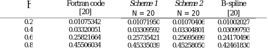
applying the techniques described in Section 2. Taking µ = 0.5 and µ = 1, in Tables 1 and 2 we compare our results with the exact solutions given in [7]. Also, in Table 3 the numerical solution obtained by Scheme 1 and Scheme 2 for µ = 5 is compared with the numerical approximation of the exact solutions given by a Fortran code [20] and the numerical solution obtained by B-spline collocation method [20]. From Tables 1−3 we see that Scheme1 and Scheme 2 yields a reasonable numerical solution for µ = 0.5, 1 and 5. As said in [20, 23], the stiffness ratio near x = 1 increases as µ increases. For this reason, most common numerical methods fail to provide enough accurate solutions for large values of µ. In Table 4 the numerical solution obtained by the Scheme 2 with N = 300, for

µ = 10, 30, is compared with the results obtained in [20] by the adaptive collocation method over a non-uniform mesh using N = 330 and those obtained in [23] by finite difference method (FDM) for mesh size N = 2000. It can be seen from Table 4 that the results obtained using Scheme 2 have a good agreement with the results obtained in [20, 23].

Table 1: Results for Troesch’s problem ( = 0.5).

x Exact Scheme1

N = 10 N = 20

Scheme2

N = 10 N = 20

0.1 0.0959443493 5.0(-10) 1.0(-10) 8.0(-10) 1.0(-10) 0.2 0.1921287477 1.0(-9) 1.0(-10) 1.4(-9) 1.0(-10) 0.3 0.2887944009 1.3(-9) 1.0(-10) 2.0(-9) 0 0.4 0.3861848464 1.7(-9) 1.0(-10) 1.0(-10) 0 0.5 0.4845471647 1.8(-9) 1.0(-10) 2.7(-9) 0 0.6 0.5841332484 1.9(-9) 1.0(-10) 2.8(-9) 0 0.7 0.6852011483 1.8(-9) 1.0(-10) 2.7(-9) 1.0(-10) 0.8 0.7880165227 1.5(-9) 1.0(-10) 2.3(-9) 1.0(-10) 0.9 0.8928542161 9.0(-9) 0 1.3(-9) 0

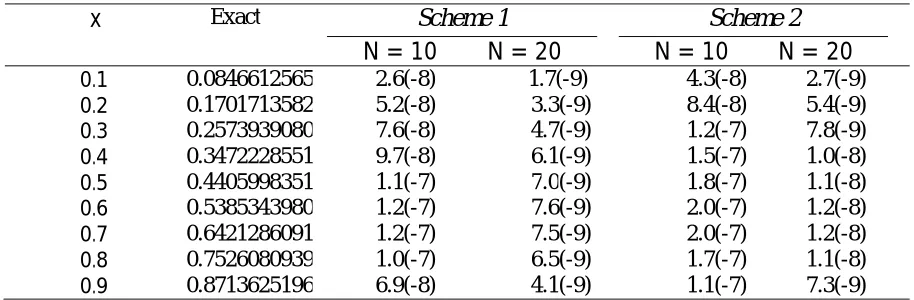
Table 2: Results for Troesch’s problem (µ = 1).

x Exact Scheme 1

N = 10 N = 20

Scheme 2

N = 10 N = 20

0.1 0.0846612565 2.6(-8) 1.7(-9) 4.3(-8) 2.7(-9) 0.2 0.1701713582 5.2(-8) 3.3(-9) 8.4(-8) 5.4(-9) 0.3 0.2573939080 7.6(-8) 4.7(-9) 1.2(-7) 7.8(-9) 0.4 0.3472228551 9.7(-8) 6.1(-9) 1.5(-7) 1.0(-8) 0.5 0.4405998351 1.1(-7) 7.0(-9) 1.8(-7) 1.1(-8) 0.6 0.5385343980 1.2(-7) 7.6(-9) 2.0(-7) 1.2(-8) 0.7 0.6421286091 1.2(-7) 7.5(-9) 2.0(-7) 1.2(-8) 0.8 0.7526080939 1.0(-7) 6.5(-9) 1.7(-7) 1.1(-8) 0.9 0.8713625196 6.9(-8) 4.1(-9) 1.1(-7) 7.3(-9)

Example 3. Consider the following singularly perturbed problem [6, 31]: −ϵy + y = x, 0≤ x≤1,

y(0) = 1, y(1) = 1 + exp 1

√ϵ .

(21)

The exact solution of this problem is

y(x) = x + exp − x √ϵ .

(22)

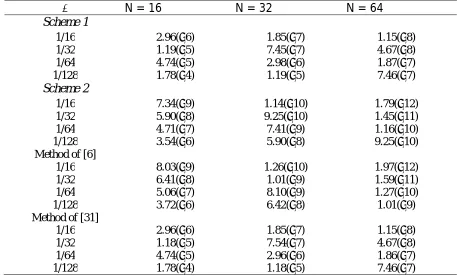
This problem is solved in [6] by sixth-order compact finite difference method. Also, in [31] the authors used quintic spline method to solve this problem. For the purpose of comparison in Table 8, we compare maximum absolute errors of our methods, for different values of ϵ and N, together with the maximum absolute errors given in [6, 31].

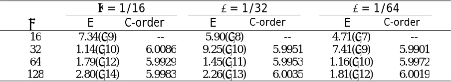
Furthermore, we have calculated the computational orders of our methods (denoted by C-order) with the following formula:

log(E )−log(E )

log(2) ,

where E and E are maximum absolute errors obtained using N and 2N mesh intervals, respectively. The results are summarized in Tables 9 and 10. From Tables 9 and 10, we see that the computational and theoretical orders of Scheme 1 and Scheme 2 are very close to each other, i.e the order of Scheme 1 and Scheme 2 are O(h ) and O(h ), respectively.

4.

C

In this paper, a new family of schemes for numerically solving two point boundary value problems is presented. We showed that, the order of Scheme 1 and Scheme 2 are O(h ) and

problem and certain singularly perturbed problem. According to the numerical results, Scheme 1 and Scheme 2 can handle these kind of problems effectively and the comparison show that the proposed methods are in good agreement with the existing results in the literature. Also numerical results confirm the theoretical results of the proposed techniques.

Table 3: Comparison of numerical solutions for Troesch’s problem (µ = 5).

Fortran code [20]

Scheme 1 Scheme 2 B-spline

N = 20 N = 20 [20]

0.2 0.01075342 0.4 0.03320051 0.6 0.25821664 0.8 0.45506034

0.01071950 0.01070406 0.01002027 0.03309592 0.03304801 0.03099793 0.25735421 0.25695699 0.24170496 0.45335039 0.45258050 0.42461830

Table 4: Comparison of numerical solutions for Troesch’s problem (µ = 10, 30).

µ = 10 µ = 30

Scheme 2 B-spline[20] FDM Scheme 2 FDM[23]

N = 300 = 330 N = 2000 N = 300 N = 2000

0 0 0 0 0 0

0.1 4.204824(−5) 4.207335(−5) 4.211194(−5) 3.614375(−13) 2.500056(−13) 0.2 1.297676(−4) 1.298517(−4) 1.299642(−4) 7.277661(−12) 5.033929(−12) 0.3 3.584358(−4) 3.586905(−4) 3.589786(−4) 1.461766(−10) 1.011094(−10) 0.4 9.764246(−4) 9.771828(−4) 9.779034(−4) 2.936036(−9) 2.030831(−9) 0.5 2.655001(−3) 2.657239(−3) 2.659022(−3) 5.897186(−8) 4.079021(−8) 0.6 7.218002(−3) 7.224571(−3) 7.228934(−3) 1.184481(−6) 8.192908(−7) 0.7 1.963429(−2) 1.965351(−2) 1.966406(−2) 2.379094(−5) 1.645584(−5) 0.8 5.364813(−2) 5.370517(−2) 5.373034(−2) 4.778560(−4) 3.305241(−4) 0.9 1.518614(−1) 1.520568(−1) 1.521140(−1) 9.614584(−3) 6.644214(−3) 0.95 2.757046(−1) 2.761735(−1) 4.460814(−2) 3.026175(−2) 0.97 3.713175(−1) 3.721473(−1) 8.991531(−2) 5.753674(−2) 0.98 4.468330(−1) 4.481030(−1) 1.441330(−1) 8.223035(−2) 0.99 5.714501(−1) 5.739404(−1) 5.218877(−1) 1.269861(−1)

1 1 1 1 1 1

Table 5: Comparison of numerical solutions for Bratu’s problem ( = 1).

Exact Scheme 1 Scheme 2 B-spline[27] IDF[30]

0.1 0.049846791245 0.2 0.089189934629 0.3 0.117609095768 0.4 0.134790253884 0.5 0.140539214400 0.6 0.134790253884 0.7 0.117609095768 0.8 0.089189934629 0.9 0.049846791245

Table 6: Comparison of numerical solutions for Bratu’s problem ( = 2).

Exact Scheme 1 Scheme 2 B-spline[27] IDF[30]

0.1 0.114410743268 0.2 0.206419116488 0.3 0.273879311826 0.4 0.315089364226 0.5 0.328952421341 0.6 0.315089364226 0.7 0.273879311826 0.8 0.206419116488 0.9 0.114410743268

0.114410743264 0.114410743265 0.1143935651 0.114410743957 0.206419116481 0.206419116483 0.2063865190 0.206419117764 0.273879311817 0.273879311820 0.2738344125 0.273879313548 0.315089364215 0.315089364220 0.3150365062 0.315089366227 0.328952421330 0.328952421335 0.3288968072 0.328952423437 0.315089364215 0.315089364220 0.3150365062 0.315089366228 0.273879311817 0.273879311820 0.2738344125 0.273879313550 0.206419116481 0.206419116483 0.2063865190 0.206419117767 0.114410743264 0.114410743265 0.1143935651 0.114410743961

Table 7: Comparison of numerical solutions for Bratu’s problem ( = 3.51).

Exact Scheme 1 Scheme 2 B-spline[27] IDF[30]

0.1 0.364335803565 0.2 0.677869705682 0.3 0.922214197098 0.4 1.078634240752 0.5 1.132617978282 0.6 1.078634240752 0.7 0.922214197097 0.8 0.677869705682 0.9 0.364335803565

0.364335803086 0.364335802967 0.357388461 0.364335803565 0.677869704751 0.677869704528 0.664283874 0.677869705683 0.922214195783 0.922214195480 0.902930838 0.922214197097 1.078634239178 1.078634238825 1.055419782 1.078634240752 1.132617976616 1.132617976246 1.107989815 1.132617978283 1.078634239178 1.078634238825 1.055419782 1.078634240752 0.922214195783 0.922214195480 0.902930838 0.922214197097 0.677869704751 0.677869704528 0.664283874 0.677869705683 0.364335803086 0.364335802967 0.357388461 0.364335803565

Table 8: Comparison of maximum absolute errors for Example 3.

ϵ N = 16 N = 32 N = 64

Scheme 1

1/16 2.96(−6) 1.85(−7) 1.15(−8)

1/32 1.19(−5) 7.45(−7) 4.67(−8)

1/64 4.74(−5) 2.98(−6) 1.87(−7)

1/128 1.78(−4) 1.19(−5) 7.46(−7)

Scheme 2

1/16 7.34(−9) 1.14(−10) 1.79(−12)

1/32 5.90(−8) 9.25(−10) 1.45(−11)

1/64 4.71(−7) 7.41(−9) 1.16(−10)

1/128 3.54(−6) 5.90(−8) 9.25(−10)

Method of [6]

1/16 8.03(−9) 1.26(−10) 1.97(−12)

1/32 6.41(−8) 1.01(−9) 1.59(−11)

1/64 5.06(−7) 8.10(−9) 1.27(−10)

1/128 3.72(−6) 6.42(−8) 1.01(−9)

Method of [31]

1/16 2.96(−6) 1.85(−7) 1.15(−8)

1/32 1.18(−5) 7.54(−7) 4.67(−8)

1/64 4.74(−5) 2.96(−6) 1.86(−7)

Table 9: Errors and computational orders obtained by Scheme 1, for Example 3.

ϵ = 1/16 E C-order

ϵ = 1/32 E C-order

= 1/64

C-order 16 2.96(−6) -- 1.19(−5) -- 4.74(−5) -- 32 1.85(−7) 3.9999 7.45(−7) 3.9975 2.98(−6) 3.9915 64 1.15(−8) 4.0078 4.67(−8) 3.9957 1.87(−7) 3.9942 128 7.26(−10) 3.9855 2.92(−9) 3.9993 1.16(−8) 4.0108

Table 10: Errors and computational orders obtained by Scheme 2, for Example 3.

= 1/16 E C-order

ϵ= 1/32

E C-order

ϵ= 1/64

E C-order

16 7.34(−9) -- 5.90(−8) -- 4.71(−7) -- 32 1.14(−10) 6.0086 9.25(−10) 5.9951 7.41(−9) 5.9901 64 1.79(−12) 5.9929 1.45(−11) 5.9953 1.16(−10) 5.9972 128 2.80(−14) 5.9983 2.26(−13) 6.0035 1.81(−12) 6.0019

A

.

R

1. H. B. Keller, Numerical Methods for Two−Points Boundary−Value Problems, Dover, New York, 1992.

2. Z. A. Majid, N. A. Azmi, M. Suleiman, Solving second order ordinary differential equation ns using two point four step direct implicit block method, Eur. J. Sci. Res.31 (2009) 29−36.

3. A. Saadatmandi, M. R. Azizi, Chebyshev finite difference method for a two-point boundary value problems with applications to chemical reactor theory, Iranian J. Math. Chem. 3 (2012) 1−7.

4. M. Dehghan, A. Saadatmandi, The numerical solution of a nonlinear system of second-order boundary value problems using the sinc-collocation method, Math. Comput. Modelling46 (2007) 1434−1441.

5. S Yeganeh, Y. Ordokhani, A. Saadatmandi, A sinc-collocation method for second-order boundary value problems of nonlinear integro-differential equation, J. Inform. Comput. Sci. 7 (2012) 151−160.

7. U. Erdugan, T. Ozis, A smart nonstandard finite difference scheme for second order nonlinear boundary value probles, J. Comput. Phys. 230 (2011) 6464−6474.

8. R. E. Mickens, Advances in the Applications of Nonstandard Finite Difference Schemes, Wiley−Interscience, Singapore, 2005.

9. P. K. Pandey, Rational finite difference approximation of high order accuracy for nonlinear two point boundary value problems, Sains Malays 43 (2014) 1105−1108.

10.P. K. Pandey, A non-classical finite difference method for solving two point boundary value problems, Pac. J. Sci. Technol.14 (2013) 147−152.

11.H. Ramos, A non-standard explicit integration scheme for initial-value problems, Appl. Math. Comput.189 (2007) 710−718.

12.E. S. Weibel, On the confinement of a plasma by magnetostatic fields, Phys. Fluids2 (1959) 52−56.

13.D. Gidaspow, B. S. Baker, A model for discharge of storage batteries, J. Electrochem. Soc. 120 (1973) 1005−1010.

14.A. Kouibia, M. Pasadas, Z. Belhaj, A. Hananel, The variational spline method for solving Troesch’s problem, J. Math. Chem.53 (2015) 868−879.

15.S. M. Roberts, J. S. Shipman, On the closed form solution of Troesch’s problem, J. Comput. Phys. 21 (1976) 291−304.

16.J. P. Chiou, T. Y. Na, On the solution of Troesch’s nonlinear two-point boundary value problem using an initial value method, J. Comput. Phys. 19 (1975) 311−316.

17.H. Temimi, A discontinuous Galerkin finite element method for solving the Troesch’s problem, Appl. Math. Comput.219 (2012) 521–529.

18.S. H. Chang, A variational iteration method for solving Troesch’s problem, J. Comput. Appl. Math. 234 (2010) 3043−3047.

19.S. H. Chang, Numerical solution of Troesch’s problem by simple shooting method, Appl. Math. Comput.216 (2010) 3303−3306.

20.S. A. Khuri, A. Sayfy, Troesch’s problem: A B-spline collocation approach, Math. Comput. Modelling54 (2011) 1907−1918.

21.A. Saadatmandi, T. Abdolahi-Niasar, Numerical solution of Troesch's problem using Christov rational functions, Comput. Methods Differ. Equ. 3 (2015) 247−257.

23.H. Temimi, M. Ben-Romdhane, A. R. Ansari, G. I. Shishkin, Finite difference numerical solution of Troesch’s problem on a piecewise uniform Shishkin mesh, Calcolo54 (2017) 225−242.

24.H. N. Hassan, M. A. El-Tawilb, An efficient analytic approach for solving two-point nonlinear boundary value problems by homotopy analysis method, Math. Methods Appl. Sci.34 (2011) 977−989.

25.A. M. Wazwaz, A reliable study for extensions of the Bratu problem with boundary conditions, Math. Methods Appl. Sci.35 (2012) 845−856.

26.J. Rashidinia, K. Maleknejad, N. Taheri, Sinc-Galerkin method for numerical solution of the Bratu’s problems, Numer. Algorithms62 (2013) 1−11.

27.H. Caglar, N. Caglar, M. Ozer, A. Valarıstos, A. N. Anagnostopoulos, B-spline method for solving Bratu’s problem, Int. J. Comput. Math. 87 (2010) 1885−1891.

28.E. Deeba, S. A. Khuri, S. Xie, An algorithm for solving boundary value problems, J. Comput. Phys.159 (2000) 125−138.

29.J. Karkowski, Numerical experiments with the Bratu equation in one, two and three dimensions, Comput. Appl. Math.32 (2013) 231−244.

30.H. Temimi, M. Ben-Romdhane, An iterative finite difference method for solving Bratu’s problem, J. Comput. Appl. Math.292 (2016) 76−82.

31.J. Rashidinia, R. Mohammadi, S. H. Moatamedoshariati, Quintic spline methods for the solution of Singularly perturbed boundary-value problems, Int. J. Comput. Methods Eng. Sci. Mech.11 (2010) 247−257.

32.A. Khan, I. Khan, T. Aziz, Sextic spline solution of a singularly perturbed boundary value problems, Appl. Math. Comput. 181 (2006) 432−439.

33.A. Saadatmandi, Z. Akbari, Transformed Hermite functions on a finite interval and their applications to a class of singular boundary value problems, Comput. Appl. Math. 36 (2017) 1085−1098.

34.A. Saadatmandi, N. Nafar, S. P. Toufighi, Numerical study on the reaction cum diffusion process in a spherical biocatalyst, Iranian J. Math. Chem. 5 (2014) 47−61.

35.T. Caraballo, M. Herrera-Cobos, P. Marín-Rubio, An iterative method for non-autonomous nonlocal reaction-diffusion equations, Appl. Math. Nonlinear Sci. 2 (2017) 73−82.

36.F. Balibrea, On problems of Topological Dynamics in non-autonomous discrete systems, Appl. Math. Nonlinear Sci. 1 (2016) 391−404.