Analysis of Delayed Prey-Predator System with Ratio-Dependent III Functional Response

(1)

Vol. 3, 2015, 59-70

ISSN: 2349-0632 (P), 2349-0640 (online) Published 15 December 2015

www.researchmathsci.org

59

Analysis of Delayed Prey-Predator System with

Ratio-Dependent III Functional Response

V.Madhusudanan1 and S.Vijaya2

1

Department of Mathematics, S.A Engineering College Email: [email protected]

2

Department of Mathematics, Annamalai University, Tamilnadu Annamalainagar-608002, email: [email protected] Received 29 November 2015; Accepted 12 December 2015

Abstract. In this paper, we proposed and analyzed a prey-predator system with discrete time delay incorporating ratio-dependent III functional response. The equilibrium of proposed system are determined and behavior of the system is investigated around equilibrium. In the presence of delay, the condition for boundedness of the system is established. Choosing delay as a bifurcation parameter, the existence of Hopf bifurcation of the system has been investigated. We also show that increasing delay may cause bifurcations into periodic solutions. Some numerical simulation has been performed to substantiate our analytical findings. .

Keywords: Prey-Predator system, discrete time delay, Ratio dependent III functional response, Hopf bifurcation.

1. Introduction

The predator-prey model forms the building block of ecosystem. The dynamical behavior of predator and its prey exhibits a variety of pattern. It paves interest for many biologists and mathematicians to develop significant models for challenging situations. A system of differential or difference equation is used to formulate a predator-prey model mathematically. The key component in the predator-prey interaction is the functional response. Generally, functional response depends on prey density. If the functional response relies on the predator-prey ratio, then such a functional response is called ratio-dependent functional response.

(2)

V.Madhusudanan and S.Vijaya

60

2. Mathematical model

Mathematical model considered is based on the predator-prey system with Ratio dependent III functional response.

2 2 2 2

2 2

1 ( )

dX X X Y

rX

dT K mY X

dY X Y

Y

dT mY X

α

β

_γ

 

=  − − ₊

 

= −

+ (1)

where

r

is the intrinsic growth rate of prey,

K

is the environmental carrying capacity of the prey,

α

_{is the maxima relative increase of predation,}

m

is the half-saturation constant,β is the conversion factor.

γ

is the death rate of predator.

In order to minimize the number of parameters involved with the model system, it is extremely useful to write the system in non-dimensionalized form. For this purpose we introduce the variables X Y, and T as follows.

x X ,y aY

K K

→ → and

t

→

Tr

In terms of the non-dimensionalized variables the model system (1) become

(

)

2 2 2

2

2 2

1 ( )

dx

cx y

x

dt

y

x

dy

dx y

ey

dt

y

x

=

−

+

=

−

+

₍₂₎

where

, ,

c d e

r r

r m

α

β

γ

= = =

The non-negative initial conditions are associated with system (2)

x≥0,y≥0 (3) The objective of this paper is to perform a qualitative analysis on this ratio dependent III functional response in the system with discrete time delay. . The paper is organized as follows: In section 3 we present some positive invariance and boundedness results. In section 4 we obtain the existence of the equilibrium points of model (2) .In section 5, we investigate local behavior of the equilibrium points in absence of delay. In section 6 analysis of the model in presence of discrete delay is discussed. In section 7 Numerical simulations are used to illustrate some of our result.

3. Positive invariance and boundedness Preliminaries

(3)

Response

61

that population ever survives. Since the resources are limited, the boundedness may depict a natural suspension to growth.

Positive invariance

Theorem 1. The positive quadrant int(R₊2) is invariant for system(2)

Proof: We prove that for all t∈[0, [, ( )Q x t >0, ( )y t >0.we show this by method of contradiction

Suppose, it is not true, there must exists one , t_q , 0< <tq Q such that

∀t∈[0, [, ( )tq x t >0, ( )y t >0

And minimum of x t( ), ( )q y tq vanish.

From the system (2), we have

1 0

2 0

( ) (0) exp ( , )

t

x t x G x y dt

y t y G x y dt

 

=  

 

 

=  

 

∫

where

1 2 2

2

2 2 2

( , ) (1 )

( , ) ( )

cxy

G x y x

x y

dx

G x y e

x y

= − − +

= −

+

Since ( , )x y are defined and continuous on [0, ]t_q there exists a L≥0 such that

[0, [q

t t

∀ ∈

1 0

2 0

( ) (0) exp ( , ) (0) exp( )

t

q

t

q

x t x G x y dt x t L

y t y G x y dt y t L

 

=  ≥ −

 

 

=  ≥ −

 

∫

It is clear that if limit t→t_q we obtain

( ) (0) exp( )

q q

x t x t L

y t y t L

≥ −

which contradicts the fact minimum of one x t( ), ( )q y tq vanish

There fore ∀t∈[0, [, ( )Q x t >0, ( )y t >0

This completes the proof.

(4)

62

4. Existence of equilibrium points

In this section we first determine the existence of fixed points of the differential equations (2) and then we investigate their stability by calculating the eigenvalues for the variational matrix (2) at each fixed point. To determine the fixed points, the equilibrium is the solution of pair of equation given below

2 2

(1 cxy ) 0

x x

y x

− − =

+ (4)

2 2 2

( dx ) 0

y e

y +x − = By simple computation of the above algebraic system, it was found that there are two non-negative fixed points

i) E₁(1, 0) is axial fixed point is always exists, as the prey population grows to the carrying capacity in the absence of predation

ii) E x2( ,y ) ∗ ∗

is the positive equilibrium point exists in the interior of the first quadrant where x [d c e d( e)]

d

∗₌ − −

and y d ex e

∗ ₌ − ∗

5. Local Stability analysis in absence of delay

In order to check the stability of the model (2), the variational matrix corresponding to each equilibrium point is calculated.

The variational matrix of equilibrium point at

E

₁

(1, 0)

is

₁ 1

0

c E

d e

− −

 

= ₋ 

 

The eigenvalues of

E

₁ are

−

1

_andd−e .Therefore the model system (2) is stable around

E

₁ ford <e for which, x−yplane is the stable. On the other hand the system is always unstable around

E

₁ if d >e which is, infact , a saddle point and whose stable manifold in x-direction and unstable in y direction ford >e Hence we state the following theorem.

Theorem 3. The equilibrium pointE₁is stable if d<e.

6. Analysis of delayed model

(5)

Response

63

realistic and importance models of population ecology should be taken into account with the time delay and the stability of an ecological systems with time delays has been studied by many authors[13-16,18-19]

In this section we analyze the model system (2) with delay

τ

(discrete time delay in predator response function).then the model system (2) takes the following form

(

)

2 2 2

2

2 2

1 ( )

(

) (

)

((

)

(

)

dx

cx y

x

dt

y

x

dy

dx t

y t

e

dt

y

t

x t

τ

=

−

+

−

=

−

− +

−

₍₅₎

With the initial densities

0( ) 1( ) 0, 0( ) 2( ) 0, r ([ , 0] ), ( , 0), 0

x

θ

=

φ θ

> y

θ

=

φ θ

>

φ

∈C −

τ

→R₊

θ

∈ −

τ

> (6)

Boundedness of the system with ττττ>0

Theorem 4. All solution of the system (5) are uniformly bounded with an ultimate

bound.

Proof: Define the function

) ( ) ( )

( y t

d c t

x

t = −τ +

ω

which on differentiation with respect to t dt dy d c t dt dx dt d + − = ( τ) ω =       − − + − − − + − + − − − − − − − ( ) ) ( ) ( ) ( ) ( ) ( ) ( ) ( ) ( ( ) ( 1 )(

( ₂ ₂

2 2 2 2 t ey t y t x t y t dx d c t y t x t y t x t x t x τ τ τ τ τ τ τ τ τ τ =













−

+

−

+













+

−

d

e

t

cy

t

x

t

x

t

y

d

c

t

x

(

τ

)

(

)

(

τ

)(

2 (

τ

))

(

)

1

≤ _      ₋ + + − d e w 4 ) 1 ( 1 2 which yields

d

e

t

w

t

4 )

1 (

1 )

(

sup

2

lim

≤

+

−

∞ →

≡ M

Then there exists positive constant M>0 such that ω(t) < M for large t.

Local stability analysis in presence of delay

Now we direct our attention due to discuss of stability of system at E1.

(6)

64    

 

− − −

= ₋

e de

c

E _λτ

0 1

1

The characteristic equation of E1 is of the form

) (

) 1

(

λ

+

λ

+e−de−λτ =0

Here λ=-1 is a negative eigenvalue we now consider the equation

λ =

de

−λτ

−

e

(7) If τ=0, and d<e, the equilibrium E1 is locally asymptotically stable. If substitute λ=iµ in

(7) and equating real and imaginary parts, we obtain,

µτ

µ

=

−

d

sin

µτ

cos

d

e

=

(8) Eliminating τ from (8) we obtain

2 2 2

e d − =

µ

(9) We know that (9) has positive root µ+ is d>e. Hence there is positive constant τ+ such that

τ>τ+, E1 becomes unstable.

The main purpose of this section to study the stability behavior of E x y₂( ,∗ ∗) in the presence of discrete delay ( τ≠ 0). Now to prove the stability behavior ofE x y2( , )

∗ ∗

for the system (5), First we linearize the system (5) by using following transformation

11 12

21 22

( ) ( ) ( )

u t a u t a v t

v t c u t

τ

c v t

τ

′ = +

′ = − + −

where

2 2 2 2 2

2 2 2 2

3 2 2

2 2 2 2

11 ₂ 12 ₂

21 ₂ 22 ₂ 22

( ) ( )

,

( ) ( )

2 2

, ,

( ) ( )

cx y x y cx x y

a x a

x y x y

dx y dx y

c c a e

x y x y

∗ ∗ ∗ ∗ ∗ ∗ ∗

∗

∗ ∗ ∗ ∗

− − −

= − + =

+ +

−

= = = −

+ +

The characteristic equation is

∆

( )

λ τ

,

=

(

λ

2

+

l

₁

λ

+

l

₂

)

+

(

l

₃

λ

+

l e

₄

)

−λτ

=

0

(10) where

1 11 22, 2 11 22, 3 22, 4 22 11 12 21

l = − −a a l =a a l = −c l =c a −a c If

τ

=0 in (10) the characteristic equation becomes

2

1 3 2 4

(l l ) (l l ) 0

λ

+ +

λ

+ + = (11) The root of (11) is

2

1 3 1 3 2 4

( ) ) 4( )

2

l l l l l l

λ

=− + ± + − + (12)

From (12), we have

λ

has negative real parts if and only if

l1+ >l3 0,l2+ >l4 0 (13)

(7)

Response

65

2

1 2 3 4

(−w +il w+l )+(il w+l )(cosw

τ

−isinw

τ

)=0

Equating real, imaginary parts we get

2

2 4cos 3 sin

w − =l l w

τ

+l w w

τ

1 3

cos

4

sin

l w

w

τ

l

w

τ

−

=

−

Squaring and adding we get (14)

4 2 2 2 2 2

1 3 2 2 4

( 2 ) ( ) 0

w +w l −l − l + l −l =

We get the roots of (14) is

2 2 2 2 2 2 2

1 3 2 1 3 2 2 4

2 ( 2 ) ( 2 ) 4( )

2

l l l l l l l l

w =− − − + − − − − (15)

It follows

2 2 1 3 2

(l − −l 2 )l >0 and (l₂2−l₄2)>0 (16) are satisfied .Hence the equation does not have any positive solutions.

We conclude the following theorem

Theorem 4. If the conditions (13) and (16) are satisfied ,then all the roots of the equation

(10) have negative real parts for all

τ

≥0.Then the equilibrium E x y₂( ∗, ∗)is stable for

τ

≥0.

Put w2 =

δ

then the equation (14) becomes

2 2 2 2 2

1 3 2 2 4

(l l 2 )l (l l ) 0

δ

+

δ

− − + − =

If (l22 −l42)<0 holds then (14) has unique positive root

δ

0 then

2 2 2 2 2 2 2

1 3 2 1 3 2 2 4

0

( 2 ) ( 2 ) 4( )

2

l l l l l l l l

δ

= − − − + − − − −

The corresponding time delay is

2 1 4 1 3 0 2 4

0 2 2 2

0 3 0 4 0

( )

1 2

cos ( l l l w l l ) k ,k 0,1, 2...

w l w l w

π

τ

₌ − − − ₊ ₌

+ Differentiate (10) with respect to

τ

(

)

1

3 1

3 4 3 4

2

( )

l l

d

d l l e λτ l l

λ

τ

λ λ

λ

−

+

 

= + −

  ₊ ₊

 

=

(

)

2

2 3 4 3

2 2

3 4 3 4

( )

l l l e l

l l e l l

λτ λτ

λ

τ

λ

−

− − + ₊ ₋

+ +

=

(

)

2

3 2

2 2 2

3 4 3 4

( ) 1

( )

l l

l l e λτ l l

λ

τ

λ

−

λ

− ₋ ₊ ₋

(8)

66

(

)

2

2 4

2 2 2

1 2 3 4

( )

l l

l l l l

λ

τ

λ λ

λ

−

= − −

− + + +

Taking λ=iw0 in above equation, we get

( )

(

)

(

( )

)

0

1 ₂

0 2 4

2 2

2

0 0 3 0 4

0 0 1 0 2

( )

( ) ( )

iw

iw l l

d i

d _λ _iw _iw _{l iw} _l i l iw l w

λ

τ

ω

− = − −   = + +   ₊   ₋ ₊ ₊

(

)

(

)

(

)

2 2

0 2 0 2 1 0

2 2 2

0 2 1 0

0 0 2 1 0

4 3 0 4

2

0 4 3 0 4 3 0 0

( ) ( ) ( ) . ( ) ( ) [ ( ) . ( ( )

w l w l i l w

w l i l w

w w l i l w

l il w

l i

w l il w l il w w

τ  ₊ ₋ ₊  =   + − + − −      ₋  +   + −   Re 0 1 iw d d _λ

λ

τ

− =       =

(

)

(

)

( )

4 2 0 2 2 ₂ 2 2

0 0 2 1 0

w l

w w l l w

  −    _ _ − +  __ __  

+ ₂ ₂4 ₂ ₂

0 4 3 0

( )

[ ]

l

w l l w

2

+

Thus we obtain

0 1 iw d Re d _λ

λ

τ

− =    

  > 0

Therefore transversality condition holds and hence hopf bifurcation occurs at

τ τ

=

₀ This signifies that there exits at least or equal value with positive real part for

τ τ

>

₀

Theorem 5. If E₂exists with the condition (14) and

δ ω

= ₀2be positive root of (14), then there exists a

τ τ

= ₀∗ such that

(i) E2 is locally asymptotically stable for 0

τ τ

0 ∗

≤ < (ii) E₂ is unstable for

τ τ

> ₀∗

(iii) The system (5) undergoes a Hopf –bifurcation around E₂ at

τ τ

= ₀∗

τ

0 min

∗ ₌ 0 ( ) h

ω

where 2 1 4 1 3 0 2 4

0 2 2 2

0 3 0 4 0

(

)

1

2 (

)

cos (

l

l l w

l l

)

k

,

0,1, 2...

h

k

w

l w

l

w

π

ω

₌

−

₊

₌

+

and the minimum taken over all positive

ω

0such that

2 0

δ ω

= is a solution of (14)

Analysis of Global Stability

(9)

Response

67

Theorem 6. The positive equilibrium point E2 of non-delayed model system (2) is

globally asymptotically stable.

Proof: Let us consider the function

H (x, y) =

xy

1

Clearly H (x, y) is positive for both x > 0, y > 0

1 2 2

2

2 2 2

( , ) (1 )

( , ) ( )

cxy

G x y x x

x y

dx

G x y y e

x y

= − −

+

= −

+ Now

) ( )

( )

,

( ₁ G₂ H

y H G x y x

∂ ∂ + ∂

∂ = ∆

(

₂ ₂

) (

2 ₂ ₂

)

2 2

1

y x

dxy

y x

x c

y x

c

y − + + ₊ − ₊

− =

=

(

)

(

)

2 2

2 2 2 2

1 y x 2dxy

c

y _x _y _x _y

 

− ₋ _ − _ ₋

 ₊  ₊

 

(

)

_ 

   

+ + − − −

= ₂

2 2

2

2 ₂

1

y x

dxy cx

cy

y

< 0

From the above equation, we note that ∆(x, y) does not change sign and is not identically zero in the interior of the positive quadrant we show that of x-y plane. In the following theorem E2 is globally asymptotically stable.

7. Numerical simulations

In this section, we present some numerical simulation result to validate our analytical findings. Let us consider the parameter of the system (2) as in appropriate units. In Fig.1(a) and Fig1(b),we take d=0.85,e=1.32,c=0.83,the Eigen values of E₁are

1 1, 2 0.47

λ

= −

λ

= − .In this case E₁ is locally asymptotically stable. From Fig 1(a) we observe that the predator is driven to extinction, where as the prey approaches the carrying capacity.Fig1 (b) phase portrait is also tends to the boundary equilibrium point (1,0).In Fig 2(a) and Fig 2(b),we take d=1.55,e=1.32,c=2.3.

In this case it satisfy the condition of theorem

2 2 2 2

1 3 1.3029,1 3 22 0.90146 0, 2 4 0.1634 0

l + =l l − −l l = > l −l = > .We conclude that

2( , )

(10)

68

1.55, 1.32, 0.6

d = e= c= the eigen values of delayed system is

λ

₁= −1,

λ

₂ =0.23.In this case E1 is unstable and the value of

τ

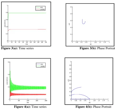
=0.613.In this case time series and phase

portrait of the system in Fig 3(a) and 3(b).If we take d=1.55,e=1.32,c=2.5,in this case prey and predator population shows periodic solutions see Fig 4(a) and phase portrait as shown in Fig 4(b).

0 20 40 60 80 100 120 140 160 180 200 0

0.2 0.4 0.6 0.8 1 1.2 1.4 1.6

time

p

o

p

u

la

ti

o

n

s

prey predator

0 0.25 0.5 0.75 1 1.25 1.5 1.75 2 0

0.1 0.2 0.3 0.4 0.5 0.6 0.7 0.8 0.9 1

x(t)

y

(t

)

Figure 1(a): Time series Figure 1(b): Phase Portrait

0 50 100 150 200 250 300 350 400 0

0.2 0.4 0.6 0.8 1

time

p

o

p

u

la

ti

o

n

s

prey predator

0 5 10 15 20 25 30 35 40 45 50 0

5 10 15 20

x(t)

y

(t

)

(11)

Response

69

0 20 40 60 80 100 120 140 160 180 200 0

0.2 0.4 0.6 0.8 1

time

p

o

p

u

la

ti

o

n

s

prey predator

0 0.25 0.5 0.75 1 1.25 1.5 1.75 2 0

0.1 0.2 0.3 0.4 0.5

x(t)

y

(t

)

0 500 1000 1500 2000 0

0.2 0.4 0.6

time

p

o

p

u

la

ti

o

n

s

prey predator

0 0.25 0.5 0.75 1 1.25 1.5 1.75 2 0

0.1 0.2 0.3 0.4 0.5 0.6 0.7 0.8 0.9 1

x(t)

y

(t

)

8. Conclusion

In this work, the local stability condition for various equilibrium points and the boundedness of the system with ratio-dependent III functional response is investigated in the absence of gestational delay. And the stability condition for the interior equilibrium points is analyzed in the presence of discrete time delay. It has been evident that the system undergoes Hopf bifurcation while choosing delay as bifurcation parameter. Also increasing the delay has caused bifurcation into periodic solution. Finally, numerical simulations have substantiated the analytical findings.

REFERENCES

1. A.F.Nindjin and M.A.Aziz Alauoui, Analysis of a predator–prey model with modified Leslie-Gower and Holling type II scheme, Non Linear Analysis: Real and World Application, 7 (2006) 1104-1118.

(12)

70

3. C.Jost, O.Arino and R.Arditi, About deterministic extinctionin ratio-dependent predator-prey models, Bull. Math. Biol., 61(1) (1999) 19-32.

4. D.Xiao and S.Ruan, Global dynamics of a ratio dependent predator-prey system, J. Math. Biol., 43(3) (2001) 268-290.

5. D.Kesh, A.K.Sarkar and A.B.Roy, Persistence of two prey-one predator system with ratio-dependent predator influence, Math. Appl. Sci., 23 (2000) 347-356.

6. G.Birkoff and G.C.Rota, Ordinary differential equations, Ginn (1982).

7. H.R.Akcakaya, R.Arditi and L.R.Ginzburg, Ratio-dependent predition: an abstraction that works, Ecology, 76 (1995) 995-1004.

8. J..F.Zhang and F.Huang, Non-linear dynamics of a delayed Leslie predator-prey model, Non linear Dynamics, 77 (2014) 1577-1588.

9. K.Gopalsamy, Stability and Oscilations in Delay Differential Equations of Population Dynamics, Kluwer Academic Publishers, Netherlands, 1992.

10. K.Wang and Y.L.Zhu, Permanence and Global asymptotic stability of delayed predator-prey model with Hassell-Varley type functional response, Bulletin of Iranian Mathematical Society, 37 (2011) 197-215.

11. P.Abrams, The fallacies of ratio-dependent predation, Ecology, 75(6) (1994) 1842-1850 .

12. P.J.Pal, P.K.Mandal and K.K.Hahiri, A delayed ratio dependent predator-prey model of interacting populations with Holling type III functional response, Nonlinear Dynamics, 76 (2014) 201-220.

13. R.Arditi and L.R.Ginzburg, Coupling in predator-prey dynamics: ratio dependence, J. Theor.Biol., 139 (1989) 311-326.

14. S.Gakkar and R.K.Naji, Chaos in three species ratio dependent food chain, Chaos, Solitons and Fractals,14 (2002) 771-778.

15. S.B.Hsu, T.W.Hwang and Y.Kuang, Rich dynamics of a ratio-dependent one prey- two predators model, J. Math. Biol., 43 (2001) 377-396.

16. S.Baek, W.Ko and I.Ahn, Coexistence of a one-prey two-predators model with ratio-dependent functional responses, Appl. Comput. Math., 219 (2012) 1897-1908. 17. S.L.Yuan and Y.L.Song, Stability and Hopfbifurcation in a delayed Leslie-Gower

predator-prey system, Journal of Mathematical Analysis and Applications, 259 (2001) 8-17.

18. Wenzhang, Haihong Liu, Bifurcating analysis for a leslie-Gower Predator-Prey System with time delay, International Journal of Non Linear Science, 15 (2013) 35-44.