http://www.sciencepublishinggroup.com/j/ajrs doi: 10.11648/j.ajrs.20180601.16
ISSN: 2328-5788 (Print); ISSN: 2328-580X (Online)
Study the Effect of New Egypt Wet Mapping Function on
Space Geodetic Measurements
Sobhy Abd Elmonam Younes
Department of Public Works Engineering, Faculty of Engineering, Tanta University, Tanta, Egypt
Email address:
To cite this article:
Sobhy Abd Elmonam Younes. Study the Effect of New Egypt Wet Mapping Function on Space Geodetic Measurements. American Journal of Remote Sensing. Vol. 6, No. 1, 2018, pp. 29-38. doi: 10.11648/j.ajrs.20180601.16
Received: January 28, 2018; Accepted: March 7, 2018; Published: March 27, 2018
Abstract:
Atmospheric water vapour degrades the accuracy of the results of space geodetic observations due to permanent electric dipole moments. It creates excess path lengths by retarding (slowing and bending) the propagation of the electromagnetic waves that are used in global positioning system (GPS) and very long baseline interferometry (VLBI) observations. It is known that the excess path lengths are less than 30~40 cm at the most, and are the primary obstacles of space geodesy because of the highly variable distribution of water vapour in the atmosphere. In this study, we compared modern five wet mapping functions by evaluating their effects on the tropospheric signal delay and position estimates in GPS data processing, and precise Egypt wet mapping function model is derived based on eight stations of radiosonde data well-distributed over and around Egypt (five stations used to estimate new model and other three as check points). To derive the new Egypt wet mapping function, the troposphere is divided into regular small layers. Ray tracing technique of actual signal path traveled in the troposphere is used to estimate tropospheric slant delay. Real GPS data of five stations (RTK-Network methods) were used for the assessment of new model against the available international models. These international models include Niell (NMF), Black & Eisner (B&EMF), Ifidas (IFMF), Hearing (HMF), and UNBabc MF. The data were processed using Bernese software version 5.0. The results indicate that the new Egypt wet MF model is the best model at Egypt region and has improved the wet tropospheric delay estimation up to 23.3 percent at five degree elevation angles.Keywords:
Radiosonde Data, Troposphere Models, GPS Data, Egyptian Meteorological Authority (EMA), Wet Mapping Function1. Introduction
GPS (Global Positioning System) has become an important tool for any endeavor where a quick measurement of geodetic position is required. However GPS observations contains both systematic and random errors. To reduce or eliminate the effect of some these biases and errors, GPS observable differencing technique, and/or linear combination between observables are formed. In addition, GPS-biases models can also be used.
The troposphere is the electrical neutral atmospheric region that extends up to 50 km from the surface of the earth. The troposphere is a non-dispersive medium for radio frequencies below 15 GHz. As a result, it delays the GPS carrier and codes identically. Unlike the ionospheric delay, the tropospheric delay can't be removed by combining GPS waves L1&L2
observations. This is mainly because the tropospheric delay is frequency independent. Tropospheric delay depends on: Pressure, Temperature, Humidity and Signal path through troposphere, the tropospheric delay is minimized at the user's zenith and maximized at horizon. The tropospheric delay results in values about 2.30 m at zenith, 9.30 m for a 15°
elevation angle, and 20-28 m for a 50 elevation angle in [1].
Tropospheric delay is a function of the satellite elevation angle and the altitude of the receiver. However, a good starting point is to define it in terms of the refractive index, integrated along the signal ray path:
1 , (1)
or in terms of the refractivity of the troposphere
The tropospheric refractivity can be partitioned into the two components, one for the dry part of the atmosphere and the other for the wet part,
, (3)
and the total tropospheric delay can be calculated according the following equation:
(4)
The total tropospheric delay (dtrop) can then be estimated
by separately considering its two constituents dry component
(ddry) and wet component (dwet). About 90% of the magnitude
of the tropospheric delay arises from the dry component, and the remaining 10% from the wet component.
The dry delay has a smooth, slowly time-varying characteristic due to its dependence on the variation of surface pressure; it can be modeled and range corrections applied for more accurate positioning results using measurements of surface temperature and pressure. However, the wet delay is dependent on water vapour pressure and is a few centimeters or less in arid regions and as large as 35 centimeters in humid regions. The wet delay parameter is highly variable with space and time, and cannot be modeled precisely with surface measurements in [2]. The zenith delay can be related to the delay that the signal would experience at different elevation angles through the use of a mapping function; the mapping function is the ratio of the excess path delay at elevation angle ( ) to the path delay in the zenith direction, so the tropospheric delay at different elevation angles (mapped tropospheric delay) can be expressed as in [3]:
∗ ∗ , (5)
where:
dzdry is zenith dry delay (m)
dzwet is zenith wet delay (m)
md(ε) is the dry mapping function (no unit)
mw (ε) is the wet mapping function (no unit)
(ε) is the non-refracted elevation angle.
Most of the geodetic-quality mapping functions use the continued fraction form. This functional form for the mapping function was first proposed by in [4] and later on further developed by [5 - 9].
The general form can be written as:
! "
#$% &' ( #$% &'#$% &'⋯.)
(6)
where:
is the elevation angle and a, b, c etc. are the mapping function parameters and may be constants or functions of other variables. All the parameters in the mapping function can be estimated by least-squares fitting with ray-tracing delay values at various elevation angles as in reference [10].
In this paper, we report on an investigation to determine the error of several wet mapping functions, including the Niell (NMF) in [9], Black & Eisner (B&EMF) in [11], Ifidas (IFMF)
in [7], Hearing (HMF) in [8], and UNBabc MF in [12], at low elevation angles as low as 5° and present a new Egypt model of wet mapping functions has a good performance in Egypt and nearly countries and also to investigate its effectiveness by calculating the wet tropospheric delay to get the improvement for stations coordinates.
This model is derived by solving the integration equation (2) in slant direction using radiosonde data of eight stations well-distributed all over geographic regions of Egypt (five stations used to estimate new model and other three stations used to check new models). Radiosonde is the balloon-borne instrument package that sends temperature, humidity, and pressure data to the ground by radio signal as in reference [13]. Radiosonde data are one of the most used and precise techniques to derive the atmospheric vertical profile. The mathematical equation of Snell’s law, in spherical coordinates for a spherical earth with a spherically layered atmosphere, used in solving the integration. It may be derived by eq: as in reference [14]:
, -, sin 1, ,-, sin 1, 2-2sin 12, (7)
where r in meters is the radius of curvature, n is group
refractive index and z is the zenith angle.
2. New Egypt Wet Mapping Function
Model Estimation
The estimation of the new Egypt wet MF is implemented in four main steps. In the first step, the available radiosonde data from the eight stations are collected and used to calculate the refractivity as a function of height.
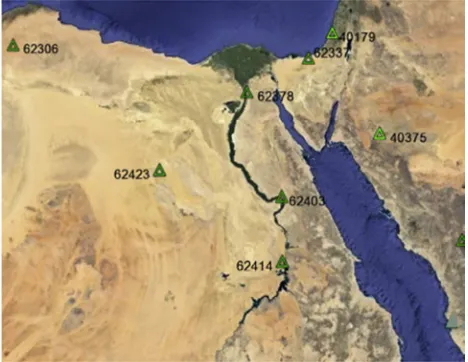
Egyptian Meteorological Authority (EMA) has 8 Upper Air stations of RDF M2K2_DC distributed in and around Egypt (see Figure 1). Code of stations and their coordinates are given also (see Table 1). Five stations used to estimate new model and other three stations used as check points. The needed data for modeling the new Egypt model are height
(H) in meter, pressure (P) in mbar, temperature (t) in C° and
humidity (e) in mbar.
Table 1. Code and approximate coordinates of the radiosonde stations.
Radiosonde station Latitude (°) Longitude (°)
40179 32.00 34.81
40375 28.38 36.60
62306 31.33 27.21
62337 31.08 33.81
62378 29.86 31.33
62423 27.05 27.96
62403 26.20 32.75
62414 23.96 32.78
In the second step, we make height regularization by assuming that the atmosphere consists of co-centric layers with the earth center as the common center. Each layer is of 20 m thickness, and the values of atmospheric modeling must be calculated at each layer. The most widely equation which represents temperature variation with height can be expressed as:
3 32 4, (8)
Where T0 is surface temperature in K°, β is temperature
lapse rate and T is temperature at each geometric height. The
vertical profile of humidity in Egypt is accurately presented as in (equation 13, in [15]):
6 62 exp 0.3838 < − 0.01919<>), (9)
where e,e0are the water vapour pressure at each layer and at
sea level respectively and H is geometric height.
Values of water vapour content at different atmospheric layers can be calculated by this formula with a mean error of 0.252 mbar and an rms of 0.067 mbar by comparing with the actual values as in reference [12].
In the third step, surfaces are fitted to provide the refractivity at any location (Φ, λ) at any specified atmospheric layer. We calculated wet refractivity with greater accuracy by Thayer in [16].
= ?> @+ ?A @B, (10)
where K2 = 64.8 K/mbar, K3 = 3.776*105 K2/mbar, e is the
water vapour pressure in mbar and T is the temperature in K.
In the fourth step we used the Simpson equation for numerical integration to calculate wet tropospheric delay at zenith angles and different elevation angles in eight radiosonde stations in different times (January, April, August, October and too average data over the year) for each stations.
2.1. Slant Delays
Slant delay is tropospheric delay at any elevation angle. We calculated wet tropospheric delay by developing Numerical Integration Model. Numerical integration model is derived for five stations (Aswan, Helwan, Mersa Matrouh, Al-arish and Qena) in (January, April, August, October and average data for one year) as follow:
Firstly, we calculated refractivity as it given by Smith and Weintraub and with greater accuracy by Thayer (as in equation 10).
Secondly, we used the Simpson's equation for numerical integration model: , ) )( ( 6 1 2 1 2 1 2 2 2 2 2 2 0
∑
∫
= = − − − + + − = n i i i i i i i i i i x x y C y B y A x x ydx n (11)where,
A
i= −
2
Q
i ;i i
i Q Q
B =2+ + 1 ;
i
i Q
C =2− 1 ;
2 2 1 2 1 2 2 − − − − − = i i i i i x x x x Q ; . 6 = +
+ i i
i B C
A
as special case of this equation, at equal intervals, then Ai = 1,
Bi = 4 and Ci =1.
At zenith the refracted path length (S) equal geometric
distance between receiver and satellite (H) and the wet
tropospheric delay can be expressed as:-
= ∑ (<>,− <>, >)( >, >+ 4 >, + >,).
,E F
B
,E (12)
At different zenith angles (z) the wet tropospheric delay is expressed as:-
∫
⇒
=
⋅
=
− s h s wetwet
N
ds
d
d
z
d
10
6sec
∫
−
=
s wet
wet
N
zdh
d
10
6sec
= ∑,E (<>,− <>, >)( >, >sec 1>, >+ 4 >, sec 1>, + >,sec 1>,).
F B
,E (13)
We used the Eq. (12) and (13) to determine wet tropospheric delay and integration nodes are distributed equally from earth surface to 14-15 Km height as below:
1-From surface to 3 Km we calculate delay every 20 m (refractivity every 10 m).
2-From 3 Km to 7 Km we calculate delay every 50 m (refractivity every 25 m).
3-From 7 Km to 10 Km we calculate delay every 100 m (refractivity every 50 m).
(refractivity every 100 m).
2.2. Mapping Function
We calculated the mapping function for each of five stations in different times of the year and average data over the year for zenith angles from 5° to 85°using the following formula:
HIJ K HIJ.
Considering the generally good performance of the mapping functions based on the continued fraction form, we adopted equation (6) as our base model and focused on the
form of the three parameters a, b, and c. In order to estimate
them, we ray-traced the refractivity profiles computed from the pressure, temperature and humidity profiles from balloon flights launched from 5 radiosonde stations in Egypt over a period of 5 years (2000- 2005). Most of the stations launched radiosondes twice daily, every day of the year.
There are total of 1815 radiosonde profiles for the selected data set. For each profile, the ray tracing was done at elevation angles of 5, 6, 7, 8, 9, 10, 11, 13, 15, 17, 20, 25, 30, 35, 40, 45, 50, 55, 60, 65, 70, 75, 80, 85 and 90° to generate wet slant delays.
From the ray tracing delay values, we produced new Egypt wet MF has a 3-term continued fraction form. From a series
of analyses, we concluded that parameter a is sensitive to the
orthometric height (H) and latitude (Φ) of the station where
as parameters b and c could be represented by constants as in
reference [10]. The least-squares estimated parameters for wet MF are:
L 10 A [0.1045 + 0.0254 < + 0.2056 cos R], (14)
b and c as in Table 2.
Table 2. Constant parameters b and c of a new model.
Mean value Min. Max. RMS
b 0.000213 -0.000367 0.000815
0.00013945
c -0.019746 - 0.173 0.1298
3. Assessment of New Mapping Function
Three steps were investigated in order to assess the performance of the new Egypt wet mapping function. In the first step, statistics of new model were tested. For wet delay values determined by the new model, relative error and average relative error were determined with wet delay by ray-traced model as standard at one of check stations that didn’t use in estimating this new model. Also, standard deviation (SD) and mean values for wet delay values were calculated for low elevation angles 20°, 15°, 10° and 5°. Regression with zero interception was also applied, slope of the regression was used to illustrate the consistency of wet delay determined with the new Egypt model to those determined by ray-traced model and also it’s coefficient of correlation (C. C.) were determined.
In the second step, we have compared it with various
modern wet mapping functions. The performance was determined by comparing the wet tropospheric delay predicted by the various mapping functions with those obtained from a highly accurate ray-traced model at different elevation angles at atmospheric conditions of Egypt (as average of eight stations data and average different five times of the year). Table 3 show the modern wet MF used in this study.
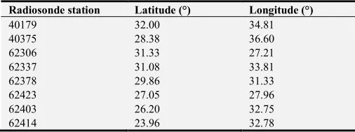
In the third step, to test the new Egypt wet model, five stations OZ95, A6, OZ97, OZ88 and E7 from Egypt network will be taken. The distances between these stations are approximately 30-40 km interval, these stations are selected from a High Accuracy Reference Network (HARN), the coordinates of these stations are shown in Table 4, GPS (Trimble 4000SSE dual frequency) is used to observe station’s coordinates and Leica Geostationary Office programme (LGO) was used for analysis the data.
Table 3. List of mapping functions.
Code Mapping functions Input parameters εmin°
NIMF Niell (1996) ε, Φ 3°
B&EMF Black & Eisner (1984) Ε 7°
IFMF Ifidas (1986) ε, t, e, P 2°
HEMF Hearing (1992) ε, t, Φ, H 3°
UNBabc Gue J. and Langley R. (2003) ε, Φ, H 2°
--- New Egypt wet MF Ε 5°
Table 4. The HARN network station’s coordinates.
Station East (m) North (m) Height (m)
OZ88 309898.5549 3303157.7225 137.729
A6 (control point) 340016.9413 3304353.5077 134.981
E7 268216.4468 3302823.793 230.875
OZ97 333921.048 3323219.2644 219.776
OZ95 350276.5655 332842.0164 230.5272
4. Results and Discussions
We calculate wet tropospheric delay using new Egypt wet MF model and compare the results with resulted wet delay from ray-traced model at low elevation angles. The statistics of the differences are investigated, see Table 5.
By analyzing data in table 5, it can be seen that the new wet MF model performs quiet well, show high consistency with ray-traced model. Relative error of the new wet MF is about from 7.37% to 10.92% and average relative error is less than 9% for all elevation angles. Regression zero interception indicates that the slope is very close to 1 from 0.95053 to 0.9535 and also coefficient correlation is very close to 1 that means the new wet MF model gives acceptable result and shows high consistency with ray-traced model in determining wet delay value in Egypt.
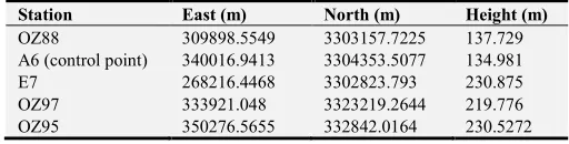
a good geographical representation for Egypt as well as a range of station heights. The overall mean biases and RMS for each mapping function at law elevation angles of 5, 7, 9,
10, 13, 15, 20, 25 and 30° are shown in Figures (2-4) and Tables (6-14).
Figure 2. Mean difference of the wet tropospheric delay mapping functions compared the ray-traced model for elevation angles from 5° to 30°.
Figure 4. Root Mean Square errors of the wet tropospheric delay mapping functions for elevation angles from 5°, 7°, 9° and 10°.
Table 5. Statistics of new Egypt wet MF comparing with ray-tracing model at one of check stations.
ε° Difference (mm) Relative error (%) slope C. C.
min max mean SD Min. Max. average
5° 115.14 173.93 140.28 71.003 7.48 10.85 8.960 0.95053 0.999979
10° 59.67 88.32 72.048 36.44 738 10.90 8.956 0.95304 0.999980
15° 40.32 59.46 48.64 24.58 7.37 10.92 8.964 0.95346 0.99998
20° 30.56 45.06 36.87 18.63 7.37 10.92 8.96358 0.953519 0.99998
Table 6. Mean difference values and RMS at 30 degree elevation angle.
M F Min. (mm) Max. (mm) Mean (mm) RMS (mm)
NMF 9.91 33.97 22.57 6.65
BE 9.92 34.02 22.51 6.62
IF 9.76 33.58 22.19 6.53
HE 9.76 33.59 22.19 6.53
UNB 9.78 33.59 22.21 6.54
New Egypt
wet 9.68 33.38 22.05 6.49
Table 7. Mean difference values and RMS at 25 degree elevation angle.
M F Min. (mm) Max. (mm) Mean (mm) RMS (mm)
NMF 11.78 40.34 26.82 7.90
BE 11.96 40.70 26.94 7.93
IF 11.61 39.89 26.37 7.76
HE 11.61 39.92 26.37 7.76
UNB 11.69 39.92 26.40 7.77
New Egypt
wet 11.45 39.40 26.07 7.68
Table 8. Mean difference values and RMS at 20 degree elevation angle.
M F Min. (mm) Max. (mm) Mean (mm) RMS (mm)
NMF 14.66 50.22 33.39 9.83
BE 15.04 51.32 33.99 10.00
IF 14.44 49.69 32.84 9.67
HE 14.45 49.74 32.84 9.67
UNB 14.48 49.74 32.89 9.68
New Egypt
wet 14.40 48.74 32.18 9.48
Table 9. Mean difference values and RMS at 15 degree elevation angle.
M F Min. (mm) Max. (mm) Mean (mm) RMS (mm)
NMF 19.71 67.40 44.82 13.20
BE 20.86 70.69 46.91 13.79
IF 19.40 66.75 44.12 12.98
HE 19.42 66.87 44.12 12.98
UNB 19.51 66.87 44.23 13.02
New Egypt
wet 18.58 64.31 42.44 12.50
Table 10. Mean difference values and RMS at 13 degree elevation angle.
M F Min. (mm) Max. (mm) Mean (mm) RMS (mm)
NMF 22.94 78.42 51.89 15.27
BE 24.83 83.79 55.41 16.28
IF 22.58 77.72 51.09 15.03
HE 22.61 77.92 51.11 15.04
UNB 22.73 77.91 51.28 15.09
New Egypt
wet 21.32 73.91 48.75 14.36
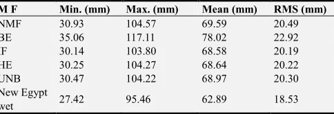
Table 11. Mean difference values and RMS at 10 degree elevation angle.
M F Min. (mm) Max. (mm) Mean (mm) RMS (mm)
NMF 30.93 104.57 69.59 20.49
BE 35.06 117.11 78.02 22.92
IF 30.14 103.80 68.58 20.19
HE 30.25 104.27 68.64 20.22
UNB 30.47 104.22 68.97 20.30
New Egypt
Table 12. Mean difference values and RMS at 9 degree elevation angle.
M F Min. (mm) Max. (mm) Mean (mm) RMS (mm)
NMF 34.61 117.88 78.46 23.10
BE 40.68 135.25 90.24 26.50
IF 33.98 117.10 77.36 22.78
HE 34.12 117.76 77.47 22.82
UNB 34.44 117.66 77.89 22.92
New Egypt
wet 30.31 105.79 69.66 20.53
Table 13. Mean difference values and RMS at 7 degree elevation angle.
M F Min. (mm) Max. (mm) Mean (mm) RMS (mm)
NMF 46.72 158.67 105.68 31.40
BE 59.62 196.13 130.95 38.44
IF 45.77 148.93 104.32 30.72
HE 46.11 159.48 104.66 30.84
UNB 46.68 159.08 105.38 31.01
New Egypt
wet 38.39 135.13 88.79 26.19
Table 14. Mean difference values and RMS at 5 degree elevation angle.
M F Min. (mm) Max. (mm) Mean (mm) RMS (mm)
NMF 71.78 246.97 161.75 47.63
BE 105.09 359.11 227.53 66.79
IF 69.97 242.27 159.87 47.13
HE 71.05 246.85 161.27 47.58
UNB 72.17 245.07 162.48 47.83
New Egypt
wet 52.25 187.2 122.46 36.17
By analyzing these results, it can be seen that for elevation angles more than 30° (zenith angles lower than 60°) the new Egypt wet MF no different more than the other MF and almost give the same results. For elevation angles low than 30° the new wet mapping function represents high accuracy in wet tropospheric delay prediction, followed by NIMF, IFMF, HEMF and UNB MF which gave nearly results. It is interesting to note that the mean accuracy of new Egypt wet MF is about 6.97 cm with rms 2.053 cm at an elevation angle of 9° and about 12.246 cm with rms 3.617 cm at 5° whereas IFMF have a 7.74 cm mean error with 2.28 cm rms at an elevation angle of 9° and 15.99 cm mean error with 4.713 cm rms even at an elevation angle of 5°. But B&EMF gave the lowest accuracy by comparing the ray-traced model since the mean error is 9.02 cm with rms 2.65 cm at an elevation angle 9° and 22.75 cm mean error with 6.68 cm rms at an elevation angle 5°.
From figures (2 to 4), we draw the following conclusions: 1) The rank by accuracy (bias – smallest to largest) is: new Egypt wet MF, IFMF, HEMF, NIMF, UNB (the differences between last four MF are small) and B&EMF.
2) At very low elevation angles (from 5° to 10°), due to the neglect of ray bending and water vapour influence, the B&E mapping function has large biases.
3) The Ifadis mapping function is the second best in accuracy, but new Egypt wet MF has improved calculating wet tropospheric delay. The improvement of the error of measurements wet tropospheric delay are presented, see
Table 15.
Results of table 15 show the improvements at elevation angles start from 5 degree until 90 degree. For the elevation angles of more than 20 degree, the different wet tropospheric delay between both models is too small and not significant. Results show that the difference between the two wet MF can be seen when the elevation angle is low up to 5 degree. New mapping function contributes 23.34 percent to estimate the wet tropospheric delay improvement percentage at five degree elevation angle.
Table 15. Percentage improvement of the error measurement for new wet delay model.
Elevation angles
New Egypt wet
MF (cm) Ifadis MF (cm) Improvement%
5° 12.25 15.98 23.34
6° 10.29 12.64 18.59
7° 8.88 10.43 14.86
8° 7.80 8.88 12.16
9° 6.97 7.74 9.94
10° 6.29 6.86 8.30
20° 3.22 3.28 1.80
90° 1.10 1.10 0.0
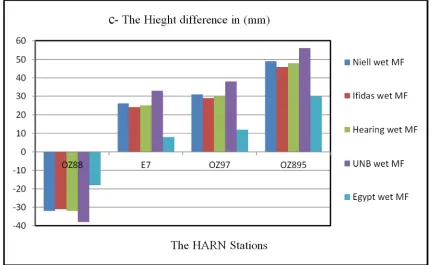
5. Effects of New Egypt Wet Mapping
Function on GPS Positioning
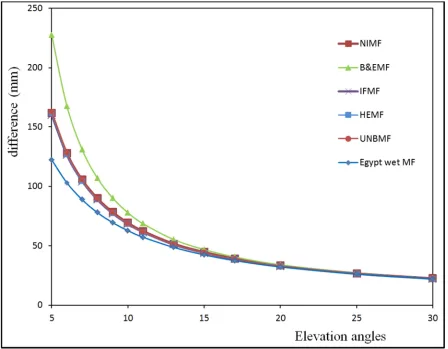
This step is used to show the differences between using the different wet mapping functions and select the model which gives the best solution where all other factors are constant. Five stations from Egypt network will be observed. These stations are selected from a High Accuracy Reference Network (HARN) have known coordinates and used GPS to measured its coordinates by RTK-network methods, under different wet tropospheric model. In this case, NMF, IFMF, HEMF, UNBMF and new Egypt wet MF models were used. In this case used new dry mapping function for Egypt to determine dry tropospheric delay as in reference [17] and for zenith wet delay used saastamoinen model with all wet MF. The results are presented in Figure 5.
Figure 5. The difference from the HARN coordinates and the observation with changing the troposphere model.
6. Conclusion
In the present research, a new precise wet tropospheric delay mapping function model is introduced. The new Egypt wet MF is based on a height and latitude of the station and elevation angles for estimating the wet component of tropospheric delay using radiosonde records. Eight stations distributed in and around Egypt are used as the input and check radiosonde data for the model calculation. The new model takes into account geometric delays as well as atmospheric asymmetry.
For the elevation angles less than 30 degrees, the reduction percentage of the new Egypt wet MF is very obvious, especially for low elevation angles. On the other hand, the reduction shows the significant improvement of the mapping function, new Egypt wet mapping function contributes 23.3 percent to the wet tropospheric delay improvement percentage at five degree elevation angle.
The test results indicate that the new Egypt wet MF model shows the best performance, compared to NMF, IFMF, B & EMF, HEMF, and UNBMF models. Five GPS stations are used to test the new model performance and results show a very significant improvement in the GPS height component can be achieved by using the new wet mapping function. This mapping function reduces errors in height determination to about 2.6 cm especially for the atmospheric conditions of Egypt and improvements in GPS horizontal component can be neglected.
Acknowledgements
The author are grateful to the staff of geodynamic
department of the National Research Institute of Astronomy and Geophysics, Helwan, Cairo, who participated in the GPS data used in this study and for allowing me to use their licensed Bernese GPS software version 5. The author thanks all members of the Egyptian Meteorological Authority for preparing, realizing and analysing the measurements of Temperature, Pressure and Humidity with different heights within their authority. The support of the department is gratefully acknowledged.
References
[1] Zarzoura F., R. Ehigiator and B. Mazurov, (2013). “Accuracy Improvement of GNSS and Real Time Kinematic Using Egyptian Network as a Case Study”, Computer Engineering and Intelligent Systems, ISSN 1719 (Paper) ISSN 2222-2863 (Online), Vol.4, No.12, 2013.
[2] Sudhir Man Shrestha, (2003). “Investigations into the Estimation of Tropospheric Delay and Wet Refractivity Using GPS Measurements”, Department of Geomatics Engineering, University of Calgary, Alberta, Canada, July, 2003.
[3] Mendes V. B. and R. B. Langely., (1994), “A comprehensive Analysis of Mapping Functions Used in Modeling Tropospheric Propagation Delay in Space Geodetic Data”. Geodetic Research Laboratory, Department of Geodesy and Geomatics Engineering, University of New Brunswick. [4] Marini, J. W., 1972. “Correction of Satellite Tracking Data for
an Arbitrary Tropospheric Profile”. Radio Science, Vol. 7, No. 2, pp. 223-231.
[6] Davis, J, L., Herring, T, A., Shapiro, I, I., Rogers, A, E, E., and Elgered, G., 1985. “Geodesy by Radio Interferometry: Effects of Atmospheric Modeling Errors on Estimates of Baseline Length”. Radio Science, Vol. 20, No. 6, pp. 1593-1607, Nov.-Dec, 1985.
[7] Ifadis, I. M., 1986. The Atmospheric Delay of Radio Waves: Modeling the Elevation Dependence on a Global Scale. School of Electrical and Computer Engineering, Chalmers University of Technology, Goteborg, Sweden, Technical Report No. 38L, pp. 115.
[8] Herring, T. A., 1992. Modeling Atmospheric Delays in the Analysis of Space Geodetic Data. Proceedings of the Symposium on Refraction of Trans-Atmospheric Signals in Geodesy, Eds. J. C. De Munck and T. A. Th. Spoelstra, Netherlands Geodetic Commission, Publications on Geodesy, No. 36, pp. 157-164.
[9] Niell, A. E., 1996. “Global Mapping Functions for the Atmosphere Delay at Radio Wavelengths”. Journal of Geophysical Research, Vol. 101, No. B2, pp. 3227-3246. [10] Guo J., and Richard B. L., (2003). “A New Tropospheric
Propagation Delay Mapping Function for Elevation Angles Down to 2. Department of Geodesy and Geomatics Engineering, University of New Brunswick, Canada.
[11] Black, H. D. and A. Eisner, 1984. “Correcting Satellite Doppler Data for Tropospheric Effects”. Journal of Geophysical Research, Vol. 89, No. D2, pp. 2616-2626.
[12] Langely, R, B., and Guo, J., 2003. A New Tropospheric Propagation Delay Mapping Function for Elevation Angles to 2°". Proceeding of ION GPS/GNSS 2003, 16th International Technical Meeting of the satellite Division of the Institute of Navigation, Portland, OR, 9-12 sep., 2003, pp 386-396. [13] Abdelfatah, M. A., Mousa, A. E., Salama, I. M. and El-Fiky,
G. S., 2009. “Assessment of tropospheric delay models in GPS baseline data analysis: a case study of a regional network at upper Egypt”. J. Civil Eng. Res. Mag. AL-Azhar Univ. 31 (4), 1143–1156.
[14] Kleijer, F., (2004). “Troposphere Modeling and Filtering for Precise GPS Leveling”. Department of Mathematical Geodesy and Positioning, Faculty of Aerospace Engineering, Delft University of Technology, Netherlands.
[15] Younes, S. A., 2016. “Modeling Investigation of Wet Tropospheric Delay Error and Precipitable Water Vapor Content in Egypt”. Egypt, J. Remote Sensing Space Sci. (2016), http://dx.doi.org/10.1016/j.ejrs.2016.05.002.
[16] Thayer, G. D., (1974), “An Improved Equation for the Radio Refractive Index of Air”, Radio Science, Vol. 9. No. 10, pp. 803-807.