Action Elimination and Stopping Conditions for the
Multi-Armed Bandit and Reinforcement Learning Problems
∗Eyal Even-Dar [email protected]
Department of Information and Computer Science University of Pennsylvania
Philadelphia, PA 19104
Shie Mannor [email protected]
Department of Electrical & Computer Engineering McGill University
H3A-2A7 Qu´ebec, Canada
Yishay Mansour [email protected]
School of Computer Science Tel-Aviv University
Tel-Aviv, 69978, Israel
Editor: Sridhar Mahadevan
Abstract
We incorporate statistical confidence intervals in both the multi-armed bandit and the reinforcement learning problems. In the bandit problem we show that given n arms, it suffices to pull the arms a total of O (n/ε2)log(1/δ)
times to find anε-optimal arm with probability of at least 1−δ. This bound matches the lower bound of Mannor and Tsitsiklis (2004) up to constants. We also devise action elimination procedures in reinforcement learning algorithms. We describe a framework that is based on learning the confidence interval around the value function or the Q-function and eliminating actions that are not optimal (with high probability). We provide a model-based and a model-free variants of the elimination method. We further derive stopping conditions guaranteeing that the learned policy is approximately optimal with high probability. Simulations demonstrate a considerable speedup and added robustness overε-greedy Q-learning.
1. Introduction
Two of the most studied problems in control, decision theory, and learning in unknown environment are the multi-armed bandit (MAB) and reinforcement learning (RL). In this paper we consider both models under the probably approximately correct (PAC) settings and study several important questions arising in this model. The first question is when can an agent stop learning and start exploiting using the knowledge it obtained. The second question is which strategy leads to minimal learning time. Since the multi-armed bandit setup is simpler, we start by introducing it and later describe the reinforcement learning problem.
The Multi-armed bandit problem is one of the classical problems in decision theory and control. There is a number of alternative arms, each with a stochastic reward whose probability distribution is initially unknown. We try these arms in some order, which may depend on the sequence of rewards
that have been observed so far. A common objective in this context is to find a policy for choosing the next arm to be tried, under which the sum of the expected rewards comes as close as possible to the ideal reward, i.e., the expected reward that would be obtained if we were to try the “best” arm at all times. One of the attractive features of the multi-armed bandit problem is that despite its simplicity, it encompasses many important decision theoretic issues, such as the tradeoff between exploration and exploitation.
The multi-armed bandit problem has been widely studied in a variety of setups. The problem was first considered in the 50’s in the seminal work of Robbins (1952) that derives strategies that asymptotically attain an average reward that converges in the limit to the reward of the best arm. The multi-armed bandit problem was later studied in discounted, Bayesian, Markovian, expected reward, and adversarial setups. (See Berry and Fristedt, 1985, for a review of the classical results on the multi-armed bandit problem.) Most of the research so far has considered the expected regret, and devised strategies for minimizing it. The seminal work of Lai and Robbins (1985) provides tight bounds as a function of the Kullback-Leibler divergence between the arms reward distribution, and a logarithmic growth with the number of steps. The bounds of Lai and Robbins (1985) were shown to be efficient, in the sense that the convergence rates are optimal. The adversarial multi-armed bandit problem was considered in Auer et al. (1995, 2002), where it was shown that the expected regret grows proportionally to the square root of the number of steps.
We consider the classical multi-armed bandit problem, but rather than looking at the expected regret, we develop PAC style bounds. The agent’s goal is to find, with high probability, a near
optimal arm, namely, with probability at least 1−δoutput anε-optimal arm. This naturally abstracts
the case where the agent needs to choose one specific arm, and it is given only limited exploration initially. Our main complexity criterion, in addition to correctness, is the number of steps taken by the algorithm, which can be viewed as pure exploration steps. This is in contrast to most of the results for the multi-armed bandit problem, where the main aim is to maximize the expected cumulative reward while both exploring and exploiting. Therefore, methods which balance between
exploration and exploitation such as softmax, and ε-greedy are not comparable to our methods.
Following our initial conference publication, a lower bound on the number of steps needed to obtain a PAC solution was developed in Mannor and Tsitsiklis (2004); it matches the upper bound we develop in this paper.
is: When is enough information gathered? When can the learning agent declare with reasonable confidence that the policy discovered is optimal, or at least approximately optimal? To summarize the differences, we are not concerned in the generic convergence rate (which must be slow), but we are rather interested in supplying rates which will be adjusted to the specific MDP parameters and as a result are much better for certain problems.
The problem of obtaining stopping conditions for learning in MDPs is a fundamental problem in RL. As opposed to supervised learning problems where typically a data set is given to the learner who has to commit to a classifier (or regressor in regression problem), in RL the decision maker can continue its interaction with the environment and obtain additional samples. The stopping rules that are currently employed in practice are based on ad-hoc rules, and may lead to premature stopping or to overly long trajectories.
When an action in a certain state can be determined to not belong to the optimal policy in an MDP, it can be discarded and disregarded in both planning and learning. This idea, commonly known as action elimination (AE), was proposed by MacQueen (1966) in the context of planning when the MDP parameters are known. In the planning case AE serves two purposes: reduce the size of the action sets to be searched at every iteration; identify optimal policies when there is a unique
optimal policy. (In value iteration this is the only way to reach optimal policy rather thanε-optimal
policy.) AE procedures are standard practice in solving large practical MDPs and are considered state-of-the-art; see Puterman (1994) for more details. We consider AE in the learning context when the model is not known a-priori.
In many applications the computational power is available but sampling of the environment is expensive. By eliminating sub-optimal actions early in the learning process, the total amount of sampling is reduced, leading to spending less time on estimating the parameters of sub-optimal actions. The main motivation for applying AE in RL is reducing the amount of samples needed from the environment. In addition to that, AE in RL enjoys the same advantages as in MDPs
-convergence rate speedup and possibility to find an optimal policy (rather thanε-optimal).
Overview of the paper
After defining the settings in Section 2, we consider the MAB problem in Section 3. We start from a naive algorithm for the MAB problem, and present two improved algorithms. The first algorithm in the bandit settings, Successive Elimination, has the potential to exhibit an improved behavior in cases where the differences between the expected rewards of the optimal arm and sub-optimal arms
are much larger thanε. The second algorithm, Median Elimination, achieves a better dependence
on the number of arms. Namely, the total number of arm trials is O(n/ε2log(1/δ)), which improves
the naive bound by a factor of log n, and matches the lower bounds given in Mannor and Tsitsiklis (2004).
In Section 4 we consider AE in RL. The underlying idea is to maintain upper and lower estimates of the value (or Q) function. When the expected upper estimate of the return of a certain action falls below the expected lower estimate of another action, the obviously inferior action is eliminated. We suggest both, a model-based and a Q-learning style AE algorithms. The upper and lower bounds are based on a large deviations inequality, so that when an action is eliminated, it is not optimal with high probability.
be-tween the upper and lower bounds of the value (or Q) function. We show that if the difference is small, then the greedy policy with respect to the lower estimate is almost optimal.
In Section 5 we present the results of several experiments with AE in toy problems as well as in non-trivial problems. Significant speedup with negligible computational overhead is observed as
compared toε-greedy Q-learning.
2. Model and Preliminaries
In this section we define the models considered in this paper. We start from the MAB model in Section 2.1. We then describe the MDP model in Section 2.2. While both models are well studied we prefer to recapitulate them in the PAC setup, to avoid confusion. We finally recall Hoeffding’s inequality which is a central tool in this work in Section 2.3.
2.1 Multi-Armed Bandit
The model is comprised of a set of arms A with n=|A|. When sampling arm a∈A a reward which
is a random variable R(a)is received. We assume that the reward is binary, i.e., for every arm a∈A
the reward R(a)∈ {0,1}(all the results apply without change if the reward is bounded in[0,1]and
in general as long as the reward is bounded with appropriate modifications). Denote the arms by
a1,···,anand pi=IE[R(ai)]. For simplicity of notations we enumerate the arms according to their
expected reward p1>p2> ... >pn.
An arm with the highest expected reward is called the best arm, and denoted by a∗, and its
expected reward r∗is the optimal reward. An arm whose expected reward is strictly less than r∗,
the expected reward of the best arm, is called a non-best arm. An arm a is called anε-optimal arm
if its expected reward is at mostεfrom the optimal reward, i.e., IE[R(a)]≥r∗−ε.
An algorithm for the MAB problem, at each time step t, samples an arm at and receives a
reward rt (distributed according to R(at)). When making its selection the algorithm may depend on
the history (i.e., the actions and rewards) up to time t−1. Eventually the algorithm must commit to
a single arm and select it.
Next we define the desired properties of an algorithm formally.
Definition 1 An algorithm is a(ε,δ)-PAC algorithm for the multi armed bandit with sample
com-plexity T , if it outputs anε-optimal arm, a′, with probability at least 1−δ, when it terminates, and
the number of time steps the algorithm performs until it terminates is bounded by T .
Remark 2 The MAB algorithm may terminate before T steps passed. The sample complexity we
consider is the complexity of the worst trajectory. The expected sample complexity (where the expectation is taken with respect to both the model and the algorithm) was considered in Mannor
and Tsitsiklis (2004). The expected sample complexity behaves likeΩ((n+log(1/δ))/ε2), which
is different than the complexity we prove below in Theorem 10. We note that the running time of the algorithm from Mannor and Tsitsiklis (2004) is not bounded in the worst case.
2.2 Markov Decision Processes
Definition 3 A Markov Decision process (MDP) M is a 4-tuple(S,A,P,R), where S is a set of the
states, A is a set of actions, Psa,s′ is the transition probability from state s to state s′when performing
action a∈A in state s, and R(s,a)is the reward received when performing action a in state s.
A strategy for an MDP assigns, at each time t, for each state s a probability for performing
action a∈A, given a history Ft−1={s1,a1,r1, ...,st−1,at−1,rt−1}which includes the states, actions
and rewards observed until time t−1. While executing a strategyπ we perform at time t action
at in state st and observe a reward rt (distributed according to R(st,at)), and the next state st+1
distributed according to Pat
st,·. We combine the sequence of rewards into a single value called the
return. Our goal is to maximize the return. In this work we focus on the discounted return, which
has a parameterγ∈(0,1), and the discounted return of policyπis Vπ=∑∞t=0γtrt, where r
t is the
reward observed at time t. We also consider the finite horizon return, Vπ=∑Ht=0rt for a given
horizon H.
We assume that R(s,a)is non-negative and bounded by Rmax, i.e., for every s,a : 0≤R(s,a)≤
Rmax. This implies that the discounted return is bounded by Vmax=Rmax/(1−γ); for the finite
horizon the return is bounded by HRmax. We define a value function for each state s, under policy
π, as Vπ(s) =IEπ[∑i∞=0riγi], where the expectation is over a run of policyπstarting at state s. We
further denote the state-action value function as using action a in state s and then followingπas:
Qπ(s,a) =R(s,a) +γ
∑
s′Psa,s′Vπ(s′).
Similarly, we define the value functions for the finite horizon model.
Letπ∗ be an optimal policy which maximizes the return from any start state. For discounted
return criterion, there exists such a policy which is deterministic and stationary (see, e.g.,
Put-erman, 1994). This implies that for any policy π and any state s we have Vπ∗(s) ≥Vπ(s), and
π∗(s) =argmax
a(R(s,a) +γ(∑s′Psa,s′Vπ ∗
(s′)). We use V∗ and Q∗ for Vπ∗ and Qπ∗, respectively.
We say that a policyπis ε-optimal ifkV∗−Vπk∞≤ε. We also define the policy Greedy(Q)as
the policy that prescribes in each state the action that maximizes the Q-function in the state, i.e.,
π(s) =argmaxaQ(s,a).
For a given trajectory let: Ts,abe the set of times in which we perform action a in state s and
Ts,a,s′ be a subset of Ts,ain which we reached state s′. Also, #(s,a,t)is the number of times action
a is performed in state s up to time t, i.e.,|Ts,a∩ {1,2,3, . . . ,t}|. We similarly define #(s,a,s′,t)as
|Ts,a,s′∩ {1,2,3, . . . ,t}|. Next we define the empirical model at time t. Given that #(s,a,t)>0 we define the empirical next state distribution at time t as
ˆ
Psa,s′ =
#(s,a,s′,t)
#(s,a,t) and R(sˆ ,a) =
∑t∈Ts,art
#(s,a,t).
If #(s,a,t) =0 the empirical model and the reward can be chosen arbitrarily. We define the
expec-tation of the empirical model as ˆIEs,s′,a[V(s′)] =∑s′∈SPˆsa,s′V(s′). To simplify the notations we omit
s,a in the notations ˆIEs′ whenever evident.
2.3 A Concentration Bound
Lemma 4 (Hoeffding, 1963) Let X be a set, D be a probability distribution on X , and f1, ...,fmbe
real-valued functions defined on X with fi : X →[ai,bi]for i=1, ...,m, where ai and bi are real
numbers satisfying ai<bi. Let x1, . . . ,xmbe independent identically distributed samples from D.
Then we have the following inequality
P " 1 m m
∑
i=1fi(xi)−
1
m m
∑
i=1Z bi
ai
fi(x)D(x) !
≥ε
#
≤ e−
2ε2m2
∑m
i=1(bi−ai)2
P " 1 m m
∑
i=1fi(xi)−
1
m m
∑
i=1Z bi
ai
fi(x)D(x) !
≤ −ε
#
≤ e−
2ε2m2
∑m
i=1(bi−ai)2.
Remark 5 We note that the boundedness assumption is not essential and can be relaxed in certain
situations. We also note that sometimes tighter bounds can be obtained using the relative Chernoff bound (Angluin and Valiant, 1979).
3. PAC Bounds for the Multi-Armed Bandit Problem
In this section we investigate an (ε,δ)-PAC algorithms for the MAB problem. Such algorithms
are required to output with probability 1−δanε-optimal arm. We start with a naive solution that
samples each arm 1/(ε/2)2ln(2n/δ) and picks the arm with the highest empirical reward. The
sample complexity of this naive algorithm is O(n/ε2log(n/δ)). The naive algorithm is described
in Algorithm 1. In Section 3.1 we consider an algorithm that eliminates one arm after the other. In Section 3.2 we finally describe the Median Elimination algorithm whose sample complexity is optimal in the worst case.
Input :ε>0,δ>0
Output : An arm foreach Arm a∈A do
Sample itℓ= 4
ε2ln(2nδ)times;
Let ˆpabe the average reward of arm a;
end
Output a′=arg maxa∈A{paˆ };
Algorithm 1: Naive Algorithm
Theorem 6 The algorithm Naive(ε,δ) is an (ε,δ)-PAC algorithm with arm sample complexity O (n/ε2)log(n/δ)
.
Proof The sample complexity is immediate from the definition of the algorithm. We now prove it
is an(ε,δ)-PAC algorithm. Let a′ be an arm for which IE(R(a′))<r∗−ε. We want to bound the
probability of the event ˆpa′ >pˆa∗.
P(pˆa′ >paˆ ∗) ≤ P ˆpa′ >IE[R(a′)] +ε/2 or ˆpa∗<r∗−ε/2
≤ P ˆpa′ >IE[R(a′)] +ε/2+P(paˆ ∗<r∗−ε/2)
where the last inequality uses the Hoeffding inequality. Choosingℓ= (2/ε2)ln(2n/δ)assures that
P(pˆa′>paˆ ∗)≤δ/n. Summing over all possible a′ we have that the failure probability is at most
(n−1)(δ/n)<δ.
3.1 Successive Elimination
The successive elimination algorithm attempts to sample each arm a minimal number of times and eliminate the arms one after the other. To motivate the successive elimination algorithm, we first assume that the expected rewards of the arms are known, but the matching of the arms to the
expected rewards is unknown. Let∆i=p1−pi>0. Our aim is to sample arm aifor(1/∆2i)ln(n/δ)
times, and then eliminate it. This is done in phases. Initially, we sample each arm(1/∆2
n)ln(n/δ)
times. Then we eliminate the arm which has the lowest empirical reward (and never sample it again).
At the i-th phase we sample each of the n−i surviving arms
O
1
∆2
n−i
−∆21
n−i+1
!
log(n
δ) !
times and then eliminate the empirically worst arm. The algorithm described as Algorithm 2 below.
In Theorem 7 we prove that the algorithm is(0,δ)-PAC and compute its sample complexity.
Input :δ>0, bias of arms p1,p2, . . . ,pn Output : An arm
Set S=A; ti= (8/∆2i)ln(2n/δ); and tn+1=0, for every arm a: ˆpa=0, i=0;
while i<n−1 do
Sample every arm a∈S for tn−i−tn−i+1times;
Let ˆpabe the average reward of arm a (in all rounds);
Set S=S\ {amin}, where amin=arg mina∈S{paˆ }, i=i+1;
end
Output S;
Algorithm 2: Successive Elimination with Known Biases
Theorem 7 Suppose that∆i>0 for i=2,3, . . . ,n. Then the Successive Elimination with Known
Biases algorithm is an(0,δ)-PAC algorithm and its arm sample complexity is
O log(n
δ) n
∑
i=21
∆2
i !
. (1)
Proof The sample complexity of the algorithm is as follows. In the first round we sample n arms
tn times. In the second round we sample n−1 arms tn−1−tn times. In the kth round (1≤k<n)
we sample n−k+1 arms for tn−k−tn−k+1 times. The total number of arms samples is therefore
t2+∑ni=2tiwhich is of the form (1).
algorithm which is similar to the naive algorithm, suppose that each arm is pulled 8/(∆2
2)ln(2n/δ)
times. For every 2≤i≤n−1 we define the event
Ei=
ˆ
p1tj ≥piˆtj|∀tjs.t.j≥i ,
where ˆpitj is the empirical value the ith arm at time t
j. If the events Eihold for all i>1 the algorithm
is successful.
P[not(Ei)] ≤ n
∑
j=iP[pnˆ tj <piˆtj]
≤
n
∑
j=i2 exp(−2(∆i/2)2tj)≤ n
∑
j=i2 exp(−2(∆i/2)28/∆2jln(2n/δ))
≤
n
∑
j=i2 exp(−ln(4n2/δ2))
≤ (n−i+1)δ2/n2≤δ
n.
Using the union bound over all Ei’s we obtain that the simplified algorithm satisfies all Ei with
probability at least 1−δ. Consider the original setup. If arm 1 is eliminated at time tj for some is
implies that some arm i< j has higher empirical value at time tj. The probability of failure of the
algorithm is bounded by the probability of failure in the simplified setting.
Next, we relax the requirement that the expected rewards of the arms are known in advance, and introduce the Successive Elimination algorithm that works with any set of biases. The algorithm we
present as Algorithm 3 finds the best arm (rather thanε-best) with high probability. We later explain
in Remark 9 how to modify it to be an(ε,δ)-PAC algorithm.
Input :δ>0
Output : An arm
Set t=1 and S=A;
Set for every arm a: ˆp1a=0;
Sample every arm a∈S once and let ˆptabe the average reward of arm a by time t;
repeat
Let ˆptmax=maxa∈Spˆtaandαt= p
ln(cnt2/δ)/t, where c is a constant; foreach arm a∈S such that ˆptmax−pˆta≥2αt do
set S=S\ {a};
end
t=t+1;
until|S|>1;
Algorithm 3: Successive elimination with unknown biases
Theorem 8 Suppose that ∆i >0 for i=2,3, . . . ,n. Then the Successive Elimination algorithm
is bounded by
O n
∑
i=2ln( n
δ∆i) ∆2
i !
.
Proof Our main argument is that, at any time t and for any action a, the observed probability ˆptais
withinαt of the true probability pa. For any time t and action a∈St we have that,
P[|pˆta−pa| ≥αt]≤2e−2α
2
tt≤ 2δ
cnt2.
By taking the constant c to be greater than 4 and from the union bound we have that with probability
at least 1−δ/n for any time t and any action a∈St,|pˆta−pa| ≤αt. Therefore, with probability
1−δ, the best arm is never eliminated. Furthermore, sinceαtgoes to zero as t increases, eventually
every non-best arm is eliminated. This completes the proof that the algorithm is(0,δ)-PAC.
It remains to compute the arm sample complexity. To eliminate a non-best arm ai we need to
reach a time tisuch that,
ˆ
∆ti=pˆ ti a1−pˆ
ti
ai≥2αti.
The definition ofαt combined with the assumption that|pˆta−pa| ≤αt yields that
∆i−2αt= (p1−αt)−(pi+αt)≥pˆ1−piˆ ≥2αt,
which holds with probability at least 1−δn for
ti=O
ln(n/δ∆i) ∆2
i
.
To conclude, with probability of at least 1−δ the number of arm samples is 2t2+∑ni=3ti, which
completes the proof.
Remark 9 One can easily modify the successive elimination algorithm so that it is (ε,δ)-PAC. Instead of stopping when only one arm survives the elimination, it is possible to settle for stopping
when either only one arm remains or when each of the k surviving arms were sampled O(1
ε2log(
k
δ)). In the latter case the algorithm returns the best arm so far. In this case it is not hard to show that the
algorithm finds anε-optimal arm with probability at least 1−δafter
O
∑
i:∆i>ε
log(δ∆n
i)
∆2
i
+N(∆,ε) ε2 log
N(∆,ε)
δ
!
,
where N(∆,ε) =|{i|∆i<ε}|is the number of arms which areε-optimal.
3.2 Median Elimination
The following algorithm substitutes the term O(log(1/δ))for O(log(n/δ))of the naive bound. The
idea is to eliminate the worst half of the arms at each iteration. We do not expect the best arm to be
Input :ε>0,δ>0
Output : An arm
Set S1=A,ε1=ε/4,δ1=δ/2,ℓ=1. repeat
Sample every arm a∈Sℓfor 1/(εℓ/2)2log(3/δℓ)times, and let ˆpℓadenote its empirical
value;
Find the median of ˆpℓa, denoted by mℓ;
Sℓ+1=Sℓ\ {a : ˆpℓa<mℓ};
εℓ+1=34εℓ;δℓ+1=δℓ/2;ℓ=ℓ+1; until|Sℓ|=1;
Algorithm 4: Median Elimination
Theorem 10 The Median Elimination(ε,δ) algorithm is an (ε,δ)-PAC algorithm and its sample complexity is
O
n ε2log
1
δ
.
First we show that in theℓ-th phase the expected reward of the best arm in Sℓdrops by at most
εℓ.
Lemma 11 For the Median Elimination(ε,δ)algorithm we have that for every phaseℓ:
P[max
j∈Sℓ
pj≤ max
i∈Sℓ+1
pi+εℓ]≥1−δℓ.
Proof Without loss of generality we look at the first round and assume that p1is the reward of the
best arm. We bound the failure probability by looking at the event E1={pˆ1<p1−ε1/2}, which is
the case that the empirical estimate of the best arm is pessimistic. Since we sample sufficiently, we
have that P[E1]≤δ1/3.
In case E1does not hold, we calculate the probability that an arm j which is not anε1-optimal
arm is empirically better than the best arm.
P[pˆj≥pˆ1|pˆ1≥p1−ε1/2]≤P[pjˆ ≥pj+ε1/2|pˆ1≥p1−ε1/2]≤δ1/3
Let #bad be the number of arms which are notε1-optimal but are empirically better than the best
arm. We have that IE[#bad|pˆ1≥p1−ε1/2]≤nδ1/3. Next we apply Markov inequality to obtain,
P[#bad≥n/2|pˆ1≥p1−ε1/2]≤
nδ1/3
n/2 =2δ1/3.
Using the union bound gives us that the probability of failure is bounded byδ1.
Next we prove that arm sample complexity is bounded by O((n/ε2)log(1/δ)).
Lemma 12 The sample complexity of the Median Elimination(ε,δ)is O (n/ε2)log(1/δ) .
1. δ1=δ/2 ; δℓ=δℓ−1/2=δ/2ℓ
2. n1=n ; nℓ=nℓ−1/2=n/2ℓ−1
3. ε1=ε/4 ; εℓ=34εℓ−1= 34
ℓ−1ε
/4
Therefore we have
log2(n)
∑
ℓ=1
nℓlog(3/δℓ)
(εℓ/2)2
= 4
log2(n)
∑
ℓ=1
n/2ℓ−1log(2ℓ3/δ) ((3
4)ℓ−1ε/4)2
= 64
log2(n)
∑
ℓ=1
n(8
9)
ℓ−1(log(1/δ)
ε2 +
log(3) ε2 +
ℓlog(2) ε2 ) ≤ 64n log(ε21/δ)
∞
∑
ℓ=1
(8
9)
ℓ−1(ℓC′+C) =O(n log(1/δ) ε2 )
Now we can prove Theorem 10.
Proof From Lemma 12 we have that the sample complexity is bounded by O n log(1/δ)/ε2
. By
Lemma 11 we have that the algorithm fails with probabilityδiin each round so that over all rounds
the probability of failure is bounded by∑log2(n)
i=1 δi≤δ. In each round we reduce the optimal reward
of the surviving arms by at mostεiso that the total error is bounded by∑ilog=12(n)εi≤ε.
4. Learning in MDPs
In this section we consider algorithms for the RL problem, which are based on the MAB algorithms presented above. We start from model-based learning in Section 4.1, where the parameters of the models are learned. We describe algorithms which are based on the successive elimination algo-rithm and provide stopping conditions for these algoalgo-rithms. In Section 4.2 we consider model-free learning and suggest a version of the Q-learning algorithm that incorporates action elimination and stopping conditions. In Section 4.3 we analyze the batched sampling setting of Kearns and Singh
(2002) and provide a mechanism that can use any(ε,δ)-MAB algorithm to enhance the performance
of the Phased Q-learning introduced in Kearns and Singh (2002). We also provide a matching lower bound.
4.1 Model-Based Learning
4.1.1 FINITE HORIZON
Let us first recall the classical optimality equations for finite horizon:
VH(s) = max
a {R(s,a) +IEs′[V
H−1(s′)]}, H>0 V0(s) = max
a R(s,a),
where VH(s) is the optimal value function for horizon H. We often abuse notation by using IEs′
instead of IEs′,a. Given the empirical model by time t we define the upper estimate Vδ, which will
be shown to satisfy for every horizon k and every state s, Vkδ(s)≥Vk(s)with high probability. For
horizon H we define:
VHδ(s) = max
a n
ˆ
R(s,a) +IEˆs′[VδH−1(s′)] +HRmax s
ln(c|S||δA|H2)
|Ts,a| o
, H>0 (2)
V0δ(s) = max
a n
ˆ
R(s,a) +Rmax
s
ln(c|Sδ||A|)
|Ts,a| o
, (3)
for some constant c≥4. Similarly to the upper bound VHδ, a lower bound may be defined where
the Rmaxis replaces by−Rmax. We call this estimate the lower estimate VHδ. The following Lemma
proves that VHδ is an upper estimation for any horizon and that VHδ is a lower estimation.
Theorem 13 We have that Vkδ(s)≥Vk(s)≥Vkδ(s)for all states s and horizons k, with probability at least 1−δ.
Proof We prove the claim by induction. For the base of the induction, by a simple use of Hoeffding
inequality we have that for every state s V0δ(s)≥maxaR(sˆ ,a)with probability 1−δ/(c|S||A|). Next
we assume that the claim holds for i≤k and prove for k+1 and for every action a. By definition
Vkδ+1(s)satisfies for every a that
Vkδ+1(s) ≥ R(sˆ ,a) +IEˆs′[Vk
δ(s′)] + (k+1)Rmax s
ln(c|S||A|δ(k+1)2)
|Ts,a|
≥ R(sˆ ,a) +IEˆs′[Vk(s′)] + (k+1)Rmax s
ln(c|S||A|δ(k+1)2)
|Ts,a| ,
where the second inequality follows from the inductive hypothesis. Note that Vk is not a random
variable, so we can bound the last expression using Hoeffding’s inequality. We arrive at:
P
ˆ
R(s,a) +IEˆs′[Vk(s′)] + (k+1)Rmax s
ln(c|S||A|δ(k+1)2)
|Ts,a| <R(s,a) +IEs′[V k(s′)]
≤e
−ln(c|S||A|δ(k+1)2)|T s,a| (k√+1)Rmax |T s,a|
!2
((k+1)Rmax)2
= δ
Therefore, we have that with high probability the following holds
Vkδ+1(s) ≥ max
a {R(s,a) +
ˆ
IEs′[Vk(s′)] +kRmax s
ln(c|S||δA|k2)
|Ts,a| }
≥ max
a {R(s,a) +IEs′[V k(s′)]} = Vk+1(s).
Using the union bound over all state-action pairs and all finite horizons k, we obtain that the
failure probability is bounded byδ/2 for c≥4. Repeating the same argument for the lower estimate
and applying the union bound completes the proof.
Consequently, a natural early stopping condition is to stop sampling whenkVH−VHk∞<ε. We do
not provide an algorithm here, however a detailed algorithm will be given in the following subsec-tion.
4.1.2 DISCOUNTEDRETURN- INFINITEHORIZON
In this subsection, we provide upper and lower estimates of the value function V for the infinite horizon case. The optimal value is the solution of the set of the equations:
V∗(s) =max
a {R(s,a) +γIEs′[V
∗(s′)]}, s∈S.
As in Subsection 4.1.1, we provide an upper value function Vδ, which satisfies with high probability
Vδ(s)≥V∗(s). We define Vtδat time t as the solution of the set of equations:
Vtδ(s) =max
a n
ˆ
R(s,a) +γIEˆs′[Vtδ(s′)] +Vmax s
ln(ct2|Sδ| |A|)
|Ts,a|) o
for some positive constant c and Qtδas:
Qtδ(s,a) =R(sˆ ,a) +γIEˆs′[Vδ(s′)] +Vmax s
ln(ct2|Sδ| |A|)
|Ts,a| .
Similarly, we define Vtδand Qtδas:
Vtδ(s) =max
a n
ˆ
R(s,a) +γIEˆs′Vδ(s′)−Vmax s
ln(ct2|Sδ| |A|)
|Ts,a|) o
Qtδ(s,a) =R(sˆ ,a) +γIEˆs′[Vtδ(s′)]−Vmax s
ln(ct2|Sδ| |A|)
|Ts,a| .
The next lemma shows that with high probability the upper and lower estimations are indeed correct.
Proof Suppose we run a value iteration algorithm on the empirical model at time t. Let Vtδ,kbe the
kth iteration of the value function algorithm at time t, and let Qtδ,kbe the associated Q-function, that
is
Qδt,k(s,a) =R(sˆ ,a) +γIEˆs′[Vtδ,k(s′)] +Vmax s
ln(ct2|Sδ||A|)
|Ts,a| .
Assume that we start with Vtδ,0=V∗. (The use of V∗ is restricted to the proof and not used in the
algorithm.) We need to prove that Qtδ(s,a)≥Q∗(s,a)for every s and a. Note that since the value
iteration converges, Qtδ,k converges to Qtδ. We prove by induction on the number of the iterations
that by taking Vtδ,0=V∗, with high probability for every k we have that Qtδ,k≥Qtδ,k−1, i.e., P[∀k Qkδ≥
Qkδ−1]≥1−ctδ2. For the basis, since V∗is not a random variable we can apply Hoeffding’s inequality
and obtain that for every state action pair(s,a)
P
n
ˆ
R(s,a) +γIEˆs′[V∗(s′)] +Vmax s
ln(ct2|Sδ||A|)
|Ts,a| <R(s,a) +γIEs′[V∗(s′)] o
≤e−ln(ct2|δS||A|)= δ
ct2|S||A|.
Since Vtδ,0(s) =V∗ we have that Qtδ,1(s,a) =R(sˆ ,a) +γIEˆs′[Vtδ,0(s′)] +Vmax r
ln(ct2|δS||A|)
|Ts,a| . Therefore,
Qδt,1≥Qδt,0with probability 1−ctδ2. For the induction step, we assume that the claim holds for i<k
and prove for k.
Qδt,k(s,a)−Qδt,k−1(s,a) = γIEˆs′[Vtδ,k−1(s′)−Vtδ,k−2(s′)].
Since Vtδ,k−1(s′) =maxaQt,k−1
δ (s′,a)we have by the induction that for every s,
Vδt,k−1(s) =max
a Q t,k−1
δ (s,a)≥maxa Qtδ,k−2(s,a) =Vδt,k−2(s).
So that Qtδ,k−Qtδ,k−1≥0. We conclude that P[Qδ≥Q∗]≥1−ctδ2. Repeating the same argument
for the lower estimate, Qδ, and applying the union bound over both and over all times completes the
proof for the appropriate c.
Input : MDP M,ε>0,δ>0
Output : A policy for M
Choose arbitrarily an initial state s0, let t=0,
and let U0={(s,a)|s∈S,a∈A}
repeat
At state st perform any action a s.t.(st,a)∈Ut
Receive a reward rt, and a next state st+1
Compute, Qδ,Qδfrom all the samples
t=t+1
Ut ={(s,a)|Qδ(s,a)≥Vδ(s)}
until∀(s,a)∈U |Qδ(s,a)−Qδ(s,a)|<ε(12−γ);
return Greedy(Qδ)
Algorithm 5: Model-Based AE Algorithm
A direct corollary from Lemma 14, is a stopping time condition to the Model-Based algorithm using the following Corollary.
Corollary 15 [ Singh and Yee (1994)] If ˜Q is a function such that|Q(s˜ ,a)−Q∗(s,a)| ≤εfor all
s∈S and a∈A. Then for all s
V∗(s)−Vπ˜(s)≤ 2ε
1−γ,
where ˜π=Greedy(Q).˜
Theorem 16 Supposed the Model-Based AE Algorithm terminates. Then the policy,π, the
algo-rithm returns isε-optimal with probability at least 1−δ.
Proof By Lemma 14 we know that with probability at least 1−δfor every s, a and time t we have
that Qδ(s,a)≤Q∗(s,a)≤Qδ(s,a). Therefore, with probability of at least 1−δthe optimal action
has not been eliminated in any state in any time t. Furthermore, any action b in state s that has not
been eliminated satisfies Q∗(s,b)−Qδ(s,b)≤Qδ(s,b)−Qδ(s,b)≤ε(1−γ)/2. The result follows
by Corollary 15.
4.2 Model-Free Learning
In this section we describe a model-free algorithm. We use two functions Qt and Qt, which provide
lower and upper estimations on Q∗, respectively. We use these functions to derive an asynchronous
algorithm, which eliminates actions and supplies stopping condition. This algorithm requires space which is proportional to the space used by Q-learning and converges under the same conditions. Let us first recall the Q-learning algorithm (Watkins, 1989). The Q-learning algorithm estimates the state-action value function (for discounted return) as follows:
Q0(s,a) = 0,
where s′is the state reached from state s when performing action a at time t, and Vt(s) =maxaQt(s,a).
Setαt(s,a) =1/#(s,a,t)for t∈Ts
′,a′
and 0 otherwise.1We define the upper estimation process as:
Q0δ(s,a) = Vmaxln(c|S||A| δ ), Qtδ+1(s,a) = (1−αt(s,a))Q
t
δ(s,a) +αt(s,a)
R(s,a) +γVtδ(s′) +β(#(s,a,t)),
where c>4 and s′ is the state reached from state s when performing action a at time t, Vtδ(s) =
maxaQ
t
δ(s,a)and the functionβ, which maintains the upper estimate interval is defined as:
β(k) =k q
k ln(ck2|S||A|/δ)−(1−1/k)q(k−1)ln(c(k−1)2|S||A|/δ)
Vmax.
Analogously, we define the lower estimate Qδas :
Q0δ(s,a) = −Vmaxln(c|S||A| δ ),
Qtδ+1(s,a) = (1−αt(s,a))Qtδ(s,a) +αt(s,a)
R(s,a) +γVtδ(s′)−β(#(s,a,t)),
where Vδ(s) =maxaQδ(s,a). We claim that these processes converge almost surely to Q∗. (The
proof appears in Appendix A.)
Proposition 17 If every state-action pair is performed infinitely often then the upper (lower)
esti-mation process, Qtδ(Qtδ), converges to Q∗with probability one.
The following Proposition claims that Qtδ upper bounds Q∗ and Qtδ lower bounds Q∗ with high
probability.
Proposition 18 With probability at least 1−δwe have that for every state action pair (s,a)and time t:
Qtδ(s,a)≥Q∗(s,a)≥Qtδ(s,a).
Proof We start by defining disjoints events such that their union is the event of Q not always being
an upper bound of Q∗. Let
Ek,s,a = {The first time for which Q is not an upper bound of
Q∗is when a is performed at state s at the kth time}.
Note that if Q does not upper bound Q∗it implies that one of the events Ek,s,aoccurred. Next we
bound the probability that an event Ek,s,a happens. Note that the only Q value that has changed
where a was performed art the kth time at state s is Q(s,a). We let t′ be the time of Ek,s,a and note
that Qt(s′,a′)≥Q∗(s,a)for any t<t′.
P(Ek,s,a) = P
Qt′(s,a)−Q∗(s,a)<0
Input : MDP M,ε>0,δ>0
Output : A policy for M
For every state action(s,a):
Q(s,a) = Vmaxln(c|Sδ||A|) Q(s,a) =−Vmaxln(c|Sδ||A|)
#(s,a) = 1
Choose an arbitrary initial state s
repeat
Let U(s) ={a|Q(s,a)≥V(s)}
choose arbitrarily action a∈U(s), perform it and observe the next state s′
Q(s,a):= (1− 1
#(s,a))Q(s,a) + 1 #(s,a)
R(s,a) +γV(s′) +β(#(s,a))
Q(s,a):= (1−#(s1,a))Q(s,a) + 1 #(s,a)
R(s,a) +γV(s′)−β(#(s,a))
#(s,a):=#(s,a) +1; s=s′
until∀s∈S ∀a∈U(s) |Q(s,a)−Q(s,a)|<ε(12−γ);
return Greedy(Q)
Algorithm 6: Model-Free AE Algorithm
= P 1
k k
∑
i=1(ri+γV ti
(si) +β(i))−Q∗(s,a)<0 !
≤ P 1
k k
∑
i=1(ri+γV∗(si) +β(i))−Q∗(s,a)<0
!
≤ c δ
|S||A|k2,
where we could apply Hoeffding’s inequality since V∗ is not a random variable. Now taking the
union bound over all pairs(s,a)and times k completes the proof for the upper estimate. A similar
argument for the lower estimate completes the proof.
We combine the upper and lower estimates to an algorithm, which eliminates sub-optimal ac-tions whenever possible. Furthermore, the algorithm supplies a stopping condition that assures a near optimal policy. The model free AE algorithm is described in Algorithm 6.
A direct corollary from Proposition 18 is a stopping condition to the model free AE algorithm. The following corollary follows from Corollary 15 and its proof is similar to the proof of Theorem 16.
Corollary 19 Suppose the Model-Free AE Algorithm terminates. Then the policy, it returns isε
-optimal with probability at least 1−δ.
4.3 MAB Phased Q-learning Algorithm
in MDPs. The setup is that of parallel sampling where the decision maker can sample every state and action pair, as opposed to the typical Q-learning setup where a single trajectory is followed. We will focus on the phased Q-learning algorithm Kearns and Singh (2002) which partitions the learning to phases. We will use a MAB black-box to perform the updates for each state and phase of the phased Q-learning algorithm. Although the parallel sampling model is not a realistic model it is often considered in theory as a relaxation of the MDP model which still captures many important aspects of the original problem; see Kearns and Singh (2002), Szepesvri and Munos (2005). The parallel sampling model can represent a situation where sampling from different states is very cheap (for example, when a simulator is available), so there is no real need to follow a single trajectory. In this case, reducing the number of samples needed for finding an optimal (or approximately optimal) policy is the main concern.
In phased Q-learning the value of Vk(s) is fixed during the kth phased and updated only at the
end of the phase. This implies that for every state and action(s,a)we can define a random variable
Ys(a)whose value is R(s,a) +γVk(s′), where R(s,a)is the random variable representing the reward
and s′is distributed using Psa,s′.
Our aim is to find, at each state, the action that maximizes the expected reward, and estimate
its expected reward, where the rewards are Ys(a). The phased Q-Learning can now be viewed
as using the naive algorithm for the MAB problem (Algorithm 1) in order to find the best arm. In the following we show how, using more sophisticated MAB algorithms, one can improve the convergence rate of the Phased Q-Learning.
Our algorithm uses any (ε,δ)-PAC Multi-armed bandit algorithm as a black box in the learning
process. In order to use the MAB algorithm B as, a black box, we define a simple interface, which requires the following procedures:
• InitB(ε,δ)- Initialize the parameters of B.
• GetArmB()- returns the arm a that B wants to sample next.
• U pdateB(a,r)- informs B the latest reward r of arm a.
• StopB(a,v)- returns TRUE if B terminates, and in such a case a is the output of B and v is its
estimated value. (We assume that on termination, with probability at least 1−δ, the arm a is
anε-optimal arm and|r∗−v| ≤ε.)
The MAB Phased Q-learning algorithm uses as a black box, an algorithm B for the MAB
prob-lem. It receives as input(ε,δ) and returns a policyπwhich is ε-optimal with probability at least
1−δ.
Suppose that we have some (ε,δ)-PAC MAB algorithm B, and assume B has arm sample
com-plexity TB(ε,δ). Namely, with probability 1−δ, algorithm B terminates after at most TB(ε,δ)and
outputs a policyπwhich isε-optimal. The following theorem computes the sample complexity of
MAB Phased Q-Learning algorithm as a function of TB.
Theorem 20 Assume B is an (ˆε,δˆ)-PAC multi-armed bandit algorithm. Then the MAB Phased
Q-Learning(ε,δ)algorithm outputs a policyπwhich isε-optimal policy with probability at least 1−δ,
and has sample complexity of
T(ε,δ) =|S|TB(εˆ,δˆ)logγ( εˆ
2Vmax
) =O
|S|
1−γln(
Vmax
(1−γ)ε)TB
ε
(1−γ)2
2 ,
δ(1−γ)
|S|ln(Vmax/ε)
Input :ε,δ>0 and B a multi-armed bandit algorithm
Output : A policy
Let ˆε=ε(1−2γ)2; n=logγ(εˆ/2Vmax) =O(ln( Vmax
(1−γ)ε)/(1−γ)); ˆδ=|Sδ|n;
Initialize for every s∈S: V0(s) =0;
for i=1 : n do
foreach s∈S do InitB(εˆ,δˆ);
repeat
a=GetArmB();
(s′,r) =sample(s,a); r′=r+γVi(s′);
U pdateB(a,r′);
until Stop(a,v) =TRUE; Vi+1(s) =v;π(s) =a; end
end
Algorithm 7: MAB Phased Q-Learning algorithm
First we show that in each phase the normkV∗−Vk∞decreases.
Lemma 21 Assume B is an (ˆε,δˆ)-PAC multi-armed bandit algorithm, and consider the MAB Phased
Q-Learning(ε,δ)algorithm using B. Then with probability at least 1−δ, for all k≤n,kV∗−Vkk∞
is bounded by 1−εˆγ+Vmaxγk.
Proof First we bound the probability that B outputs an arm which is notε-optimal. We bound the failure probability by using the union bound on all the invocations of B. There are
|S|n=|S|logγ(εˆ/Vmax) =O |S|ln ( Vmax
(1−γ)ε)
1−γ
!
initializations of algorithm B and for each invocation the failure probability is bounded byδ/|S|n.
Thus, the failure probability is at mostδ.
Next, we show that the error contracts in every phase. We compare the value vector, Vk, with the
standard value iteration value vector ˆVk for the case of a known model (at the end of the k-th step).
Formally,
ˆ
Vk+1(s) =max
u {IE[R(s,u)] +γIEs′[
ˆ
Vk(s′)]},
where s′ is distributed according to Psu,s′ and ˆV0=0.
We show by induction on the number of phases, that dk=kVk−Vˆkk∞≤ 1−εˆγ. The base of the
induction, t=0, for every state s we have d0=|V0(s)−Vˆ0(s)|=0. We assume that the induction
assumption holds for t<k and prove for k. Let ms,adenote the number of times the state action pair
(s,a)was sampled in the k-th iteration.
|Vk(s)−Vk(s)ˆ | =
maxu [
1
ms,u ms,u
∑
i=1−max
a [IE[R(s,a)] +γ
∑
s′Psa,s′Vkˆ−1(s′)]
≤ max
ρ∈{−ε,ˆˆε}
maxu [IE[R(s,u)] +γ
∑
s′Psu,s′Vk−1(s′)] +ρ −max
a [IE[R(s,a)] +γ
∑
s′Psa,s′Vˆk−1(s′)]
≤ εˆ+max
a γ
∑
s′
Psa,s′(Vk−1(s′)−Vˆk−1(s′))
≤ εˆ+γdk−1 ≤ εˆ+γ( εˆ
1−γ) =
ˆ
ε
1−γ.
To conclude the proof note that for the value iteration we have thatkVˆk−V∗k∞≤γkVmax, where
ˆ
V0=0 (see, e.g., Bertsekas and Tsitsiklis, 1995).
Lemma 22 When the MAB Phased Q-Learning algorithm terminates, the policy π it returns is
ε-optimal with probability at least 1−δ.
Proof By Lemma 21 we have that with probability at least 1−δ the difference kVk−V∗k∞≤
ˆ
ε
1−γ+Vmaxγk. Since ˆε=ε(1−γ)2/2, we have thatkVk−V∗k∞≤ε(1−γ)/2+Vmaxγk. The lemma
follows from our choice of n=logγ(ε(1−γ)/2Vmax).
We can now complete the proof Theorem 20.
Proof The correctness follows from Lemma 22. We bound the sample complexity as follows. By
definition, the MAB Phased Q-Learning algorithm samples at each state and action during every
phase TB(εˆ,δˆ). By definition of the algorithm, the number of phases is n=O(ln(Vmax/εˆ)/(1−γ)),
and each phase is composed from|S|MAB instances. This completes the bound on the sample
complexity.
Applying the multi-armed bandit algorithms described in the previous sections we derive the following corollary. We show that by using the median elimination algorithm, the arm sample
complexity can be reduced by a factor of log(|A|).
Corollary 23 Let B be the median elimination algorithm. MAB Phased Q-Learning algorithm has
sample complexity
T(ε,δ) =O
|S| |A|Vmax2 (1−γ)5ε2 ln(
Vmax (1−γ)ε)ln(
|S|ln(Vmax/ε) δ(1−γ) )
.
Next we introduce an almost matching lower bound. Let us introduce some more notation before we proceed. Let T denote the time until an RL algorithm stops (this may be in general a random
number). For a given RL algorithm L and a given MDP L we denote by IEL,M the expectation with
Theorem 24 Let L be a learning algorithm for MDPs under the parallel sampling model. There
are constants C1,C2,ε0,δ0,γ0such that for everyε∈(0,ε0),δ∈(0,δ0), andγ∈(0,γ0)if L returns
an ε-optimal policy with probability of at least 1−δfor every MDP with discount factor γthere
exist an MDP M for which:
IEL,M[T]≥C1 |
S| |A| (1−γ)2ε2log
C2
δ
=Ω
|S| |A| (1−γ)2ε2log(
1
δ)
.
Proof Consider the following construction which was used in Theorem 1 of Mannor and Tsitsiklis
(2004) for the MAB problem. A MAB problem with |A|arms is given. We enumerate the arms
from 0 to|A| −1, and fix ˆε>0. In each of the states one of the following hypotheses is true:
H0: r(0) =1/2+εˆ; r(i) =1/2 (i=1,2, . . . ,|A−1|),
and forℓ=1,2, . . . ,|A| −1:
Hℓ: r(0) =1/2+εˆ; r(i) =1/2 (i=1,2, . . . ,|A−1|,i6=ℓ); r(ℓ) =1/2+2ˆε.
Let IEℓbe the expectation given than hypothesis Hℓis true, and A(s)the event that the algorithm errs
in state s. In Lemma 4 in Mannor and Tsitsiklis (2004) it was proved that there are constants c1and
c2 such that for ˆε<εˆ0every algorithm that can identify the true hypothesis with probability 1−δˆ
for all the hypotheses must satisfy that:
IE0[T]≥c1|
A| −1 ˆ
ε2 log(
c2
ˆ
δ). (4)
We create the following set of MDPs. In each possible MDP there are|S|states and|A|actions in
each state. All the states are absorbing and have one of the above A hypotheses per state. The reward
in each state behaves according to H0 or one of the Hℓ. (There are|A||S| possible MDPs.) We set
ˆ
ε=2(1−γ)ε. We run algorithm L until termination. When L terminates it returns a policy which is
ε-optimal with probability of at least 1−δ. Since every state is absorbing, and by our choice of ˆε,
it implies that the right hypothesis was found in all states. Note that even if L returns a randomized policy, we will determine that the action with the highest reward is the best one (this is the reason
for the factor of 2 in determining ˆε). By taking the sum of Eq. (4) over all states we obtain that
IEL,M[T]≥c1|
A| −1 ˆ
ε2 |S|log(
c2
δ).
The result follows by an appropriate choice of constants.
5. Experiments
In this section we show four types of MDPs in which the number of samples used by AE procedures
is significantly smaller than the number of samples used by standard Q-learning andε-greedy
Q-learning. Both model free AE algorithm and standard Q-learning choose the action in each state
uniformly at random. In our experiments we focused on the steady state norm (L1 weighted by
steady state probabilities) rather than the L∞norm to emphasize the average behavior. We note that
1. A queueing system. The MDP represents a queueing problem that appears in Differentiated Services (Aiello et al., 2000, Kesselman et al., 2004). The basic settings are that the arriving packets have different values and they are buffered in a FIFO queue before being sent. The major constraints are that we reject or accept a packet upon its arrival (no preemption) and that the buffer has limited capacity. We have analyzed a queue of size five and three different
packets values, 1,20,150. In each time unit we either receive a packet or send a packet
according to some distribution. We modeled the queueing problem via a discounted MDP
with discount factorγ=0.99. The AE model-free algorithm2was compared withε-greedy
Q-learning with epsilon varying from 0.05 to 0.2. In Figure 1 we present the results forεwhich
was empirically best,ε=0.1. In this experiment we used a fixed step size. We focused here
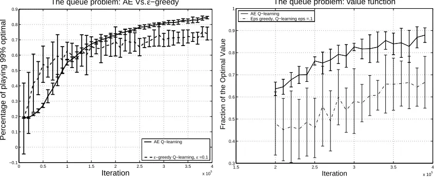
on the fraction of times in which optimal actions were performed and on the value function criterion. The results are demonstrated in Figure 1, in which we see that not only AE has better results but the variance in the results is much smaller in both the fraction of times that almost optimal actions were performed and in the value function. Figure 2 demonstrates the elimination rate of the AE procedure.
0 0.5 1 1.5 2 2.5 3 3.5 4
x 105 −0.1
0 0.1 0.2 0.3 0.4 0.5 0.6 0.7 0.8 0.9
Iteration
Percentage of playing 99% optimal
The queue problem: AE Vs. ε−greedy
AE Q−learning
ε−greedy Q−learning, ε =0.1
1.5 2 2.5 3 3.5 4
x 105 0.3
0.4 0.5 0.6 0.7 0.8 0.9 1
The queue problem: value function
Iteration
Fraction of the Optimal Value
AE Q−learning Eps greedy, Q−learning eps =.1
Figure 1: Example of a Queue of size 5 with three types of packets with values 1,20,150. The
discount factor is set to 0.99. We disregard the full queue state in which every action is
optimal. We repeated each experiment 15 times and the error bars represent 1 standard deviation.
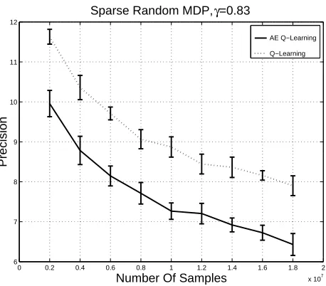
2. Random MDPs. Two types of random MDPs were randomly generated. In both types there were 20 states and 50 actions in each state. The first type is due to Puterman (1994) and is a sparse MDP, such that each action can reach only three states. The second type of random MDPs is dense, such that the next state distribution is randomly chosen for each state-action pair and might include all states. For both MDPs the immediate reward expectation is
ran-domly chosen in the interval [0,10]. Results of ten runs are presented by Figure 3 for the
0 0.5 1 1.5 2 2.5 3 3.5 4 x 10⁵ 0.1
0.2 0.3 0.4 0.5 0.6 0.7 0.8 0.9 1
The queue problem: Elimination Progress
Number of Samples
Fraction of valid actions
Figure 2: Example of a Queue of size 5 with three types of packets with values 1,20,150. The
discount factor is set to 0.99. This figure demonstrates the elimination rate. We repeated
each experiment 15 times and the error bars represent 1 standard deviation.
0 0.2 0.4 0.6 0.8 1 1.2 1.4 1.6 1.8 2
x 107 6
7 8 9 10 11 12
Number Of Samples
Precision
Sparse Random MDP, γ=0.83
AE Q−Learning
Q−Learning
Figure 3: Example of a 20 state sparse randomly generated MDPs with 50 actions in each state,
whereγ=0.833 (as in Puterman (1994).) The precision is the distance of the Q-function
from the optimal Q-function. We repeated each experiment 10 times and the error bars represent 1 standard deviation.
0 0.2 0.4 0.6 0.8 1 1.2 1.4 1.6 1.8 2 x 10⁷ 28
29 30 31 32 33 34 35 36 37 38
Number Of Samples
Precision
Dense Random MDP, γ =0.9
AE Q−Learning
Q−Learning
Figure 4: Example of a 20 state dense randomly generated MDPs with 50 actions in each state,
γ=0.9. The error bars represent 1 standard deviation.
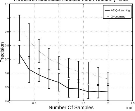
3. Howard’s automobile replacement problem. This MDP represents another realistic problem— Howard’s automobile replacement problem Howard (1960). This problem contains 40 states, in each state there are 41 actions. See Howard (1960) for a detailed description. This problem was considered as a benchmark by several authors in the optimization community. We used
the model free AE algorithm for this problem with discount factorγ=0.833 against standard
Q-learning and the results appear in Figure 5. A significant improvement is evident.
0 0.5 1 1.5 2 2.5
x 107 0.4
0.5 0.6 0.7 0.8 0.9 1 1.1
Number Of Samples
Precision
Howard’s Automobile Replacement Problem, γ=0.83
AE Q−Learning
Q−Learning
Figure 5: Example of Howard’s Automobile Replacement Problem, where the discount factor,γ, is