Optimising Kernel Parameters and Regularisation Coefficients for
Non-linear Discriminant Analysis
Tonatiuh Peña Centeno [email protected]
Neil D. Lawrence [email protected]
Department of Computer Science The University of Sheffield
Regent Court, 211 Portobello Street Sheffield, S1 4DP, U.K.
Editor: Greg Ridgeway
Abstract
In this paper we consider a novel Bayesian interpretation of Fisher’s discriminant analysis. We re-late Rayleigh’s coefficient to a noise model that minimises a cost based on the most probable class centres and that abandons the ‘regression to the labels’ assumption used by other algorithms. Opti-misation of the noise model yields a direction of discrimination equivalent to Fisher’s discriminant, and with the incorporation of a prior we can apply Bayes’ rule to infer the posterior distribution of the direction of discrimination. Nonetheless, we argue that an additional constraining distribution has to be included if sensible results are to be obtained. Going further, with the use of a Gaussian process prior we show the equivalence of our model to a regularised kernel Fisher’s discriminant. A key advantage of our approach is the facility to determine kernel parameters and the regularisation coefficient through the optimisation of the marginal log-likelihood of the data. An added bonus of the new formulation is that it enables us to link the regularisation coefficient with the generalisation error.
1. Introduction
Data analysis typically requires a preprocessing stage to give a more parsimonious representation of data, such preprocessing consists of selecting a group of characteristic features according to an optimality criterion. Tasks such as data description or discrimination commonly rely on this prepro-cessing stage. For example, Principal Component Analysis (PCA) describes data more efficiently by projecting it onto the principal components and then by minimising the reconstruction error, see e.g. (Jolliffe, 1986). In contrast, Fisher’s linear discriminant (Fisher, 1936) separates classes of data by selecting the features1 that maximise the ratio of projected class means to projected intraclass variances.
The intuition behind Fisher’s linear discriminant (FLD) consists of looking for a vector of com-pounds w such that, when a set of training samples are projected on to it, the class centres are far apart while the spread within each class is small, consequently producing a small overlap between classes (Schölkopf and Smola, 2002). This is done by maximising a cost function known in some contexts as Rayleigh’s coefficient, J(w). Kernel Fisher’s discriminant (KFD) is a nonlinearisation
that follows the same principle but in a typically high-dimensional feature space
F
. In this case, the algorithm is reformulated in terms of J(α), whereαis the new direction of discrimination. The theory of reproducing kernels in Hilbert spaces (Aronszajn, 1950) gives the relation between vectors w andα, see Section 5.1. In either case, the objective is to determine the most ‘plausible’ direction according to the statistic J.Mika et al. (1999) demonstrated that KFD can be applied to classification problems with com-petitive results. KFD shares many of the virtues of other kernel based algorithms: the appealing interpretation of a kernel as a mapping of an input to a high dimensional space and good perfor-mance in real life applications, among the most important. However, it also suffers from some of the deficiencies of kernelised algorithms: the solution will typically include a regularisation coefficient to limit model complexity and parameter estimation will rely on some form of cross validation. Unfortunately, there is no principled approach to set the former, while the latter precludes the use of richer models.
In this paper we introduce a novel probabilistic interpretation of Fisher’s discriminant. Classical FLD is revised in Section 2 while an alternative noise model is outlined in Section 3. We build on the model in Section 4 by first applying priors over the direction of discrimination to develop a
Bayesian Fisher discriminant and later we use a Gaussian process prior to reformulate the problem.
In Section 5, we compare our model to other approaches. We explore the connections of our model to the expected generalisation error in Section 6. Section 7 details an EM-based algorithm for estimating the parameters of the model (kernel and regularisation coefficients) by optimising the marginal log likelihood. We present the results of our approach by applying it on toy data and by classifying benchmark data sets, in Section 8. Finally we address future directions of our work in Section 9.
2. Fisher’s Discriminant Analysis
As mentioned above, discriminant analysis involves finding a vector of compounds w∈Rd×1 for which class separation will be maximised according to some defined statistic. Considering a set of training data and labels,
D
= (X,y) =x(n),y(n) N
n=1∈R
N×(d+1), the discriminant reduces the
dimensionality of the data through a linear combination, such that a set of single variates µ1,σ21
, µ0,σ20 is produced; where we define µq,σ2q
as the sample mean and variance of each projected group. The hope is that both groups will be distinguished from one another by using this new set. Fisher was the first to conclude that the compounds should be given by maximising the ratio of between to within class variances,
J=(µ1−µ0) 2 σ2
1+σ20
. (1)
We will use the following definitions. A vector of projections is generated by taking the product f=Xw∈RN×1and the sample means for each class are m
q=Nq−1∑n∈Nqx
(n)
q , hence the projected
mean and variance are given by
µq = Nq−1wTmq
and
σ2
q =
∑
n∈Nq
wTx(qn)−µq
2
=
∑
n∈Nq
f(n)−µq
2
, (3)
respectively. Abusing the notation, we have split the training data into two disjoint groups(X,y) = (X0,y0)∪(X1,y1), with y(
n)
q ∈ {0,1}. The coefficient Nqis the cardinality of each group, q∈ {0,1}.
Modern texts on pattern recognition and machine learning (Fukunaga, 1990; Duda and Hart, 1973; Bishop, 1995; Ripley, 1996) prefer to make explicit the dependence of this statistic on the vector of compounds. Hence, with some manipulation and the introduction of a couple of matrices we arrive at
J(w) = w
TΣ Bw
wTΣ ww
, (4)
whereΣB= (m1−m0) (m1−m0)TandΣw=∑q∈{0,1}∑
Nq
n=1
x(qn)−mq x(qn)−mq
T
,are between and within covariance matrices respectively. Matrix ΣB measures the separation between class
means whileΣwgives an estimation of the spread around them. A solution for this problem consists
of taking the derivative of Equation 4 w.r.t. w and solving. This leads to a generalised eigenvalue problem of the formΣ−w1ΣBw=λw, withλbeing the eigenvalues. A solution for the discriminant
can also be derived from geometric arguments. Given a test point x?, the discriminant is a hyper-plane D(x?) =wTx?+b, that outputs a number according to the class membership of the test point, where b is a bias term. In this context w is a vector that represents the direction of discrimina-tion. Following this line, the solution w∝ Σ−w1(m0−m1)is sometimes easier to interpret than the eigenvalue problem.
As it was demonstrated by Mika (2001), a more detailed analysis of FLD allows it to be cast as a quadratic programming problem. In order to do so, we observe that the magnitude of the solution is not relevant, so for example, the numerator of Equation 1 can be fixed to an arbitrary scalar while the denominator is minimised. In other words, the variance of the projections is minimised while the distance between projected means is kept at, say d=µ0−µ1. Rayleigh’s statistic can then be written as J=d2 σ21+σ2
0
. The subsequent discussion will make use of this ‘average distance’ constraint to reformulate the discriminant problem.
3. Probabilistic Interpretation
We introduce some notation that will be used throughout the rest of the paper. The set of variables
D
= (X,y)∈RN×(d+1)is observed or instantiated, f∈RN×1 is a dependent or latent variable and t∈RN×1 is a vector of targets that have been observed as well. The random variables will follow some probability law and in this model, in particular, we study the relationship between observed and latent variables: the noise model. From Section 2, we know that every observation inD
is projected into a single variate that ideally can take only two values which are the projected class centres, where the variance around the projections tries to be minimised. We define the parametersprocess, it is convenient to define some auxiliary variables as well, t1 is a vector filled with c1’s whenever y(n)=1 and filled with zeros otherwise; t0 is a vector filled with c0’s whenever y(n)=0 and with zeros otherwise. We also take y1=y and y0 =1−y and denote by ˆv the maximum likelihood estimate of a vector/scalar v.
3.1 The Noise Model
Figure 1 models the causal relationship between the observations
D
and the variables f and t, such that the distribution p(f,t|D
,)can be decomposed into noise model p(t|y,f) and prior p(f|X), disregarding the parameterβ. For the moment, we will ignore the prior and consider only the noise model. In graphical notation every fully shaded circle corresponds to an observed variable and a blank circle indicates a latent variable. We make use as well of partially shaded circles to indicate the binary nature of the discriminant, that is, that targets should only take one of two different values. In Figure 1 the variable t1(n)is observed whenever y(n)=1; and t0(n), whenever y(n)=0. Both variables t0and t1are discrete, with each of their elements being given by the class centres c0and c1, nevertheless, we will make a Gaussian2approximation such that every element tq(n)∼N
f(n),β−1
. From this approximation the noise model can be defined as
p(t|y,f,β) = β
N 2 (2π)N
2 exp
(
−β
2q∈{
∑
0,1}(tq−f)T
diag(yq) (tq−f)
)
. (5)
t f
X
y
0 1
1 0
y
t β
Figure 1: The proposed graphical model for discriminant analysis. The graph models the joint distribution over the latent variables f and the targets t=t0∪t1, which have been decomposed into their two
possible types. Disregarding the parameterβ, the joint probability is factorised as p(f,t|D) = p(t|y,f)p(f|X), where the noise model is given by p(t|y,f)and the prior by p(f|X). Note that we express the labels into two different groups y0 and y1. Shaded nodes indicate instantiated
variables, blank ones correspond to latent variables and partially shaded (t0 and t1) nodes are
only observed according to the values of the labels (y0 and y1, respectively). We assume that
every observed target is distributed according to tq(n)∼N
f(n),β−1, whereβis the precision
parameter.
As it can be observed from both the figure and Equation 5, there is a conditional independence assumption on the observed targets given y and f; in other words, the noise model can be further
2. We use the notationN(x|m,Σ)to indicate a multivariate Gaussian distribution over x with mean m and covariance
decomposed as p(t|y,f) = p(t0|y0,f)p(t1|y1,f), where we have disregarded the dependence on β.
We can substitute every element tq(n)by its class centre cqand take the log of (5) to obtain
L
(f,β) = −β2
N
∑
n=1
y(n)
c1−f(n)
2
+1−y(n) c0−f(n)
2
+C, (6)
where C=N 2log
β 2π.
Note that the class centres can be made to coincide with the labels. In such a ‘regression to the labels’ scheme, FLD can be recovered in a straightforward manner.
3.1.1 MAXIMUMLIKELIHOOD
Parameter estimates can be found by zeroing the gradient of
L
with respect to each f(n)andβand solving the resulting expressions for each parameter. This leads to the fixed point equationsˆ
f(n)=1−y(n)
c0+y(n)c1 (7)
and
ˆ
β= N
∑N
n=1yn c1−f(n)
2
+∑N
n=1(1−yn) c0−f(n)
2. (8)
However, the values of the class centres c0and c1are not known, so
L
can also be maximised w.r.t. them to obtainˆ
cq= 1
Nq Nq
∑
n=1y(qn)f(n)for q∈ {0,1}. (9)
The results ˆf(n)and ˆcqsuggest applying an iterative scheme to find the maximum. This can be done by substituting ˆf(n)and ˆcqon the right hand sides of Equations 9 and 7, respectively, initialising one
of the variables to an arbitrary value and updating all of them until convergence.
3.2 Model Equivalence
We now turn to the connections between Rayleigh’s statistic and the proposed noise model. In particular, we want to show that maximum likelihood learning in our framework is equivalent to maximisation of Rayleigh’s coefficient. In order to do so, we back substitute the values ˆcq into
L
(Equation 6) compute the gradient w.r.tβand solve the resulting expression forβ. The substitution of each class centre by their most probable values is indispensable and central to our framework. As a result of this substitution we can create a cost function that reduces the error around the most probable class centres. The solution forβleads to an expression of the form
ˆ
β= N σ2
1+σ20
,
quotient mentioned before, J=d2 σ21+σ2 0
, hence we can write
J(f) =d 2βˆ
N . (10)
It is clear that this quantity monotonically increases over the domainR+ because ˆβcan only take positive values. Meanwhile the likelihood, the exponential of Equation 6, expressed in terms of the estimate ˆβtakes the form
L(f) = βˆ
N/2
(2π)N/2exp
−N
2
, (11)
which is monotonic as well on this estimate.
Therefore, as Equations 10 and 11 are monotonic in ˆβ, their maximisation with respect to this parameter must yield equivalent results.
3.3 Parametric Noise Model
In this section we make two modifications to Equations 5 and 6 in order to parameterise the noise model. First, the vector of targets t is replaced by a new vector filled with the estimates ˆcqsuch that
ˆt=ˆt0∪ˆt1is generated. Second, every latent variable is related to the observations via a vector of parameters w. In a linear relation this is expressed by the inner product f(n)=wTx(n). Therefore after making these changes the log-likelihood becomes
L
= −β2
N
∑
n=1
y(n)
ˆ
c1−wTx(n)
2
+1−y(n) cˆ0−wTx(n)
2
+C. (12)
Thus a new probabilistic model is obtained, which is depicted in Figure 2.
0
y y1
0
^t ^t1
X w β
Figure 2: Partially modified graphical model for discriminant analysis. In comparison with Figure 1, the latent variable f has been replaced by a vector of parameters w. Ignoring the parameterβ, the graph factorises the joint distribution p ˆt,wD
with the product p ˆtD,w
×p(w), whereD= (X,y)
is the training data; ˆt=ˆt1∪ˆt0, the modified targets and y0and y1are the class labels. The log
of the noise model p ˆtD,w
is expressed in Equation 12 while the prior p(w)is specified in Section 4.
Furthermore, we look not only to parameterise the latent variables, but the class centres as well. Equation 9 can be used to this purpose, substituting every f(n) in it with their parametric versions wTx(n) leads to ˆcq= 1
Nq∑
Nq
n=1y
(n)
the summation and leave a quantity that we recognise to be the sample mean for class q, which we express as mq. Hence we can write ˆcq=wTmq. Therefore the log of the new noise model can be
expressed as
L
= −β2
N
∑
n=1
y(n)wTm1−wTx(n)
2
+1−y(n) wTm0−wTx(n)
2
+C. (13)
As it will be seen in Section 5, most models make the assumption that class centres and class labels coincide, that is cq=yq; including the least squares support vector machine of Suykens and
Vandewalle (1999). However this approach is suboptimal because there is no guarantee that class centres should map perfectly with the labels. Instead of following this ‘regression to the labels’ assumption, we have preferred to make use of the maximum likelihood estimates of the class centres. As we saw above, by taking this step, the class centres can be parameterised as well.
3.3.1 MAXIMUMLIKELIHOOD
Maximisation of this new form of
L
(Equation 13) has to be carried out in a slightly different way to the one presented in Section 3.1.1. Previously, the class centres were parameters which we knew beforehand were separated by some given distance. However, their parameterisation implies that the separation constraint must be considered explicitly. We therefore introduce a Lagrange multiplier to force the projected class centres to lie at a distance d, leading to the following functionΛ(w,λ) =
−β2 N
∑
n=1
y(n)
wTm1−wTx(n)
2
+1−y(n) wTm0−wTx(n)
2
+λ
wT(m0−m1)−d+C.
A solution for this constrained optimisation problem is given by
ˆ w=λ
βΣ−w1(m0−m1), with
λ=dβh(m0−m1)TΣ−w1(m0−m1)
i−1
.
Therefore, by letting∆m=m0−m1, we can express the solution as ˆ
w= dΣ− 1
w ∆m
∆mTΣ−w1∆m, (14)
which is equivalent to that produced by FLD up to a constant of proportionality (see Section 2). This completes the discussion of an alternative noise model for FLD. The new probabilistic formulation is based on a noise model that reduces the error around the class centres, instead of the class labels. Furthermore, we were interested on parameterising not only the latent variables in the model but also the centres themselves. Through the introduction of a Lagrange multiplier we saw that a constrained maximisation of the new likelihood was equivalent to standard FLD.
unattended. First we complete the study of Figure 2 by incorporating a prior over the parameters,
p(w), and later study the model of Figure 1 under the assumption that the prior, p(f|X), is a Gaussian process.
4. Bayesian Formulation
One of the aims of discriminant analysis is to determine the group membership of an input x?outside the training set. From a probabilistic perspective this process is only possible if a noise model and a prior distribution have been identified. Then the posterior over the parameters p(w|
D
)can be found as well as the corresponding predictive distribution. The posterior distribution is important because it summarises the knowledge gained after having observed the training set. The application of a Bayesian probabilistic approach offers some intrinsic advantages over other methods, for example the ability to compute ‘error bars’ and, in the context of our model, the possibility to introduce Gaussian process priors in a natural way.This section will show that the introduction of a separable Gaussian prior over w leads to a posterior distribution that is not enough to recover FLD’s solution. Later on, it will be argued that an additional step is required to ensure the equivalence is achieved. This additional step will also include the distance constraint previously implemented through a Lagrange multiplier.
4.1 Weight Space Formulation
So far we have found a maximum likelihood estimate of the parameters’ vector (see Equation 14). Now what we seek is a distribution over this vector which is obtained by combining the noise model with a prior distribution through Bayes’ rule,
p w|ˆt,
D
= p ˆt
D
,w
p(w)
p ˆt
D
,
where we have used
D
to indicate the training set(X,y)and have omitted the dependence onβ. A common choice of prior is a separable Gaussian, p(w) =N
w|0,A−1, whith zero mean and diagonal covariance A−1. The combination of this prior with the parametric noise model of Equation 13 gives a posterior of the formp(w|ˆt,
D
) ∝ exp(
−β2 N
∑
n=1
y(n)
wTm1−wTx(n)
2
+. . .
1−y(n) wTm0−wTx(n)
2
−12wTAw
. (15)
In order to obtain a complete expression for p(w|
D
) it is necessary to define the normalisation constant. As the expression is quadratic in w we know the posterior distribution will be Gaussian. However, it is still necessary to specify the mean and covariance of the distribution. In order to do so, Bayesian methods take advantage of an important property of Gaussians: if two sets of variables are Gaussian, like ˆt and w, then the conditional distribution of one set conditioned on the other is Gaussian as well. On the RHS of (15), we look to condition variable w on ˆt. The process simply consists of considering the variable ˆt as being given and on grouping terms in w. This leads to a Gaussian posterior of the formwith zero mean and covariance matrix B=βXTLX+A, where
L=I−N1−1y1y1T−N0−1y0yT0. (16) The posterior obtained is not equivalent to FLD because the mean of w is zero. In consequence, the posterior mean projection of any x? will collapse to the origin. Nonetheless, this formulation yields a consistent result if we consider that standard discriminant analysis exhibits a sign symmetry for the vector w, hence the average is zero. What our new model is missing is the incorporation of the distance constraint. In Section 3.3.1, knowledge about the variable d was incorporated to the noise model in the form of a Lagrange multiplier. We look to do the same again but in a Bayesian approach this requires that we deal with every variable in terms of probability distributions.
We propose to use the posterior p(w|
D
)as the prior for a new model that is depicted in Figure 3. In the new formulation, d is considered an extra random variable that has been observed and that depends on the distribution over w|D
. From the figure we can deduce that the joint factorises asp(d,w|
D
,γ) =p(d|D
,w,γ)p(w|D
), withγbeing a positive parameter. Note that this time we have madeD
= ˆt,X,y.d
D
γ
w
Figure 3: Graphical model to constrain the projected distance d. The graph specifies the distribution
p(d,w|D,γ)which is composed by the distributions p(w|D) and p(d|D,w,γ). The former is the posterior over the direction of discrimination, described in Section 4.1, and the latter is the constraining distribution, defined in Equation 17.
One of our main concerns is to keep the model tractable at all stages, but we are also interested in having a realistic representation of the discriminant. In order to guarantee both conditions we assume d is Gaussian with infinite precisionγ,
p(d|
D
,w,γ) =limγ→∞ γ1
2
√2πexp
−γ
2 d−w
T∆m2
. (17)
We can see that this distribution introduces the same effect as the Lagrangian of Section 3.3.1 by placing all its mass at the point d=µ0−µ1when the limitγ→∞is taken.
The process to determine a posterior p(w|
D
,d)is based on combining p(w|D
)with p(d|D
,w,γ)and then conditioning w on d. However, a final step needs to be added to work out the limit to elim-inate the dependence overγ. As a partial result, the conditional distribution p(w|
D
,d,γ) will beN
(w|w¯,Σ)with mean¯ w=lim
γ→∞γdΣ∆m, and covariance
Σ=lim
γ→∞ B+γ∆m∆m
T−1
With some algebraic manipulations and the application of the Morrison-Woodbury formula (Golub and Van Loan, 1996) we can arrive to the desired result. See Appendix A for the detailed derivation. After taking the limit, the resulting distribution will be a Gaussian
p(w|
D
,d) =N
(w|w¯ ,Σ)with parameters
¯
w = dB− 1∆m ∆mTB−1∆m and
Σ = B−1−B
−1∆m∆mTB−1 ∆mTB−1∆m .
Noticing that B=βXTLX+A, the mean of the new posterior coincides with the maximum
likeli-hood solution of Section 3.3 when an improper prior is used (i.e. A=limα→∞αI). Note that the matrixΣis positive semidefinite and therefore not invertible, this is a consequence of the fact that any vector w which does not satisfy the constraint imposed by the distribution p(d|
D
,w,γ)has a posterior probability of zero. Nevertheless, variances associated with the posterior projections can still be computed by applyingvar wTx
=xTB−1x−x
TB−1∆m∆mTB−1x ∆mTB−1∆m , which will be zero if the point x is on the direction of∆m.
The Bayesian approach we have outlined leads to a posterior distribution over the direction of discrimination which can be used to compute expected outputs and their associated variances for any given input x. However, the limitation imposed by applying a linear model is a strong one. There is an extensive amount of literature explaining why linear models are not always convenient. A common solution is to use a set of nonlinear basis functionsφsuch that the new function is linear in the parameters but nonlinear in the input space f =wTφ(x), see for example (Ruppert et al., 2003) and (Bishop, 1995). However the problem is shifted to that of specifying which and what number of basis functions to use. In the next section we shall consider the alternative approach of placing a prior directly over the vector of projections f, such that we will be working with a possibly infinite amount of basis functions. This approach will lead to a regularised version of kernel Fisher’s discriminant and ultimately to an alternative strategy to select model parameters.
4.2 Gaussian Process Formulation
The choice of a Gaussian probability measure over functions has been justified by the study of the limiting prior distribution in the neural network case when the number of hidden units ‘reaches’ infinity, (Neal, 1996). A Gaussian process (GP) is a type of stochastic process that is defined by a mean and a covariance function. By stochastic process we understand that a countable infinite set of observations{f1, . . . , fN}has been sampled from a common probability distribution.
this regard, a covariance function (or kernel) measures a priori the expected correlation between any two pair of points x(n)and x(m)in the training set. For example, in a function parameterised as
f(n)=wTφ
x(n)
,
with a prior over w specified by a spherical Gaussian with zero mean, p(w) =
N
w|0,α−1I, the implied correlation between two points is
E
h
f(n),f(m)
w
i
=α−1φx(n)
T
φ
x(m)
.
In other words, provided that the product is positive and symmetric, the correlation between the two points will lead to a Mercer kernel; see (Schölkopf and Smola, 2002). However, under these circumstances it no longer makes sense to talk about a prior over the vector w, but rather a prior over instantiations of the functions is considered.
4.2.1 PREDICTIONOVER ATESTPOINT
In order to adopt GP’s we need to go back to the formulation of the discriminant presented in Figure 1. In this figure the graph models the joint distribution p(f,t|
D
)with the product of noise modelp(t|y,f)and prior p(f|X). In this section we need to make two assumptions before doing any kind of prediction. First of all, the joint distribution over every instance f belonging to the training set or not will be a multivariate Gaussian, that is a GP. Secondly, we will continue to work with the maximum likelihood estimates of the class centres, which were denoted ˆcq. In other words, if we
use Equation 9 to form a vector ˆt and substitute it into Equation 5 we will obtain the distribution
p ˆty,f
.
Following the steps of the previous section, we could work out the posterior distribution p f|ˆt,
D
.
However, this is not what we are looking for because what we truly want is to make predictions out of new test data. Therefore, what we seek ultimately is the distribution p(f?|
D
,d), where the dis-tance variable d has been included. In order to do so, first we propose to compute the joint distribu-tion p ˆt,d,f+y,γ
, where the variable f+is given by an extended vector of the form f+=fT,f?T,
with f? being a point outside the training set. Second, the distribution p(f?|
D
,d) can be found from p ˆt,d,f+y,γ
by marginalising out the variables f and conditioning the resulting distribution on the variables ˆt and d. Lastly, the dependence on the parameterγcan be eliminated by taking the limitγ→∞.
This process is facilitated if the joint distribution is factorised into well known factors. For example, p ˆt,d,f+
y,γ
, can be given by the product of noise model, p ˆt|y,f
; Gaussian process prior p(f+); and constraining distribution p(d|y,f,γ). Firstly, the modified noise model is defined
in terms of f by applying the values of ˆcqand rearranging, (see Appendix B). The result is
p ˆt|y,f ∝
exp
−β
2f
TLf
, (18)
with L defined in Equation 16. Secondly, let the augmented vector f+be correlated with a covariance
matrix K+∈R(n+1)×(n+1), then the prior is a GP of the form
p(f+)∝exp
−12fT+K−+1f+
For future reference, the inverse of K+is partitioned as
K−+1 =
C c cT c?
,
with
c? = k?−kTK−1k−1, c = −c?K−1k,
C = K−1+c?K−1kkTK−1.
Note that the vector k∈RN×1is filled with scalars k(n)=K x(n),x
for x∈
X
.Finally, the model still needs to consider that projected class means must be separated by the dis-tance d. The introduction of a constraining distribution of the form of Equation 17 is what is needed. We can express this distribution in terms of f by replacing the term wT∆m inside the exponential by fT∆ˆy, where∆ˆy=N0−1y0−N1−1y1. Therefore the constraint becomes
p(d|y,f,γ) =lim
γ→∞ γ1
2
√2πexp−γ 2 d−f
T∆ˆy2
. (20)
Hence we can write the marginal distribution (after marginalisation of f)as
p f?,ˆt,d y,γ
=
Z
p ˆty,f
p(d|y,f,γ)p(f+)∂f.
This is a Gaussian integral that can be solved straightforwardly by applying (for example) the ma-terial on exponential integrals (Bishop, 1995) that we present in Appendix C. After conditioning f? on both ˆt and d, the solution is a Gaussian of the form
p(f?|
D
,d,γ)∝exp(
− 1
2(σ?)2 f
?−f¯?2 )
with mean
¯
f?=lim
γ→∞−γd(σ ?)2
cTQ−1∆ˆy.
and variance
(σ?)2 =lim
γ→∞ c?−c
TQ−1c−1
,
where we have defined the matrix Q=βL+C+γ∆ˆy∆ˆyT.
Just as in Section 4.1, the dependence onγis eliminated by taking the limit asγ→∞. This procedure is detailed in Appendix C. The parameters of the distribution are
¯
f?= dk
TA−1K∆ˆy
and
(σ?)2
=k?−kT K−1−D−1
k, (22)
with the matrices
D=A−1−A−1K∆ˆy ∆ˆyTKA−1K∆ˆy−1∆ˆyT
KA−1−1 and
A=βKLK+K. (23)
The predictive mean is given by a linear combination of the observed labels, in this case ex-pressed by∆ˆy. Additionally, the predictive variance is composed by two terms, one representing the test point and the other representing the observed data. These results are similar to those of typical GP regression, described in (Williams, 1999). The scheme proposed above will be termed Bayesian Fisher’s discriminant (BFD) to facilitate its referencing.
5. Relationship with Other Models
There are several well known connections between discriminant analysis and other techniques. In the statistics community, FLD is equivalent to a t-test or F-test for significant difference between the mean of discriminants for two sampled classes, in fact, the statistic is designed to have the largest possible value (Michie et al., 1994). In this section, however, we prefer to explore the connections of our approach to some algorithms that have been applied to machine learning problems, namely kernel Fisher’s discriminant and the least-squares and proximal support vector machines.
5.1 Kernel Fisher’s Discriminant
The algorithm known as kernel Fisher’s discriminant consists of a two stage procedure. The first consists of embedding the data space
X
into a possibly infinite dimensional reproducing kernel Hilbert spaceF
via a kernel function k. The second simply consists of applying FLD in this new data space. As the second stage is exactly the same as standard linear discriminant, many of the properties for FLD observed inX
will hold also inF
; for example, some form of regularisation needs to be included. However there is an extra effort involved in preparing the original data for a new data representation in the induced space, namely in terms of the kernel function.Data embedding is carried out by applying a non-linear transformationφ:
X
→F
that induces a positive definite kernel function. From the theory of reproducing kernels (Aronszajn, 1950) it is well known that the vector of compounds is a weighted combination of the training samples, such that w=∑Ni=1α(i)φ x(i). The application of this property plus the decomposition of the kernel into its spectrum:
k(x,x0) =
d
∑
i=1λiφi(x)φi x0
leads to the formulation of the Rayleigh coefficient in the feature space. Following the path of other kernel methods, the novelty in (Mika et al., 1999) resides in defining the kernel function directly and working without any reference to the spectral-based formulation.
as the rule D(x?) =∑N
i=1α(i)k x?,x(i)
+b with the coefficientsα(i)’s being obtained as the solution of maximizing a new form of the statistic
J(α) =α TMα
αTNα.
Where M=mF0 −mF1 mF0 −mF1
T
, N=KLK and mFq =Nq−1Kyq. Just as in FLD, in KFD the ‘within scatter’ matrix is not full rank. This implies that some form of regularisation will need to be applied when inverting N and this will generally be done by applying Nδ=N+δC, with C being the identity or the kernel matrices. Therefore the solution can be computed by either solving a generalised eigenproblem or by taking
αKFD∝(N+δC)−1
mF0 −mF1
. (24)
We are now in position to show the equivalence of KFD and our scheme, BFD.
Demonstration Disregarding the bias term, the projection of a new test point under KFD will be
¯
f?=αT
KFDk. (25)
Our claim is that Equation 21 is equivalent to Equation 25. In other words, that the projection of a new test point in KFD is equal to the mean of the predictive distribution for a test point under BFD. As in both equations the vector k is the same, we can write Equation 21 as
¯
f?=αTBFDk,
with the vector
αBFD∝dA−1K∆ˆy (26)
and the constant of proportionality being given by the denominator of (21). Then our proof reduces to showing that the coefficientsαKFDandαBFDare the same.
On one hand, we start by analysing KFD’s main result which is given by Equation 24. From the definition of mFq, the difference
mF0 −mF1
can be written as K∆ˆy, with∆ˆy= N0−1y0−N1−1y1, and by regularising N with a multiple of the kernel matrix we obtain
αKFD∝ KLK+β−1K
−1K∆ˆy
,
where β−1 is the regularisation coefficient.
On the other hand, substituting the value of A (Equation 23) into Equation 26, premultiplying byβ and ignoring d we get
αBFD∝ KLK+β−1K
−1K∆
ˆy,
which clearly is the regularised version of KFD that we were talking about.
As an additional insight, we observe that the coefficientsαBFDhave an equivalentαKFDif and
5.2 Least Squares Support Vector Machines
A least squares support vector machine (LS-SVM) implements a two-norm cost function3and uses equality constraints instead of the inequalities present in the standard SVM (Vapnik, 1995). This greatly simplifies the way to obtain the solution as the resulting system of equations is linear. Un-fortunately the sparseness which is characteristic of the SVM is lost. LS-SVM’s have been related to ridge regression with modified targets, discriminant analysis in the feature space (KFD) and, as many other kernelised algorithms, to GP’s.
Given a set of training data
D
= (X,y) with labels y(i)∈ {−1,1}∀i, the primal optimisationproblem for an LS-SVM is expressed as
min C=µ 2w
Tw+ζ
2
N
∑
n=1
e(n)
2
s.t. e(n)= y(n)−wTx(n) ∀n,
with µ andζbeing positive coefficients. This formulation in particular was given by Van Gestel et al. (2002) to elaborate the Bayesian framework of the LS-SVM. Such framework is nothing else but the recognition that the primal problem implements a regularised least squares cost function with regression to the labels. This cost function arises from the model depicted in Figure 4. In this figure, the joint distribution over labels and parameters factorises as p(y,w|X) =p(y|X,w)×p(w), with noise model p(y|X,w) =
N
Xw,ζ−1Iand prior p(w) =
N
0|µ−1I.y
X µ w
ζ
Figure 4: LS-SVM noise model assumes a regularised least squares cost function. The model depicted can be interpreted as the joint distribution p(y,w) =p(y|X,w)p(w), whereby the noise is Gaussian,
p(y|X,w) =N Xw,ζ−1I
, as is the prior p(w) =N 0|µ−1I
. In this model the targets and the labels are the same t≡y.
It is clear from the figure that LS-SVM employs a different noise model than BFD. In practice, the regression to the labels assumption can work well. However, it suffers from the fundamental missconception that the class labels±1 have to coincide with the projected class centres cq. The
main difference with our algorithm is that the LS-SVM assumes that targets and labels are the same, t≡y, but we do not.
Van Gestel et al. (2002) were aware of this limitation4 and relaxed the assumption t≡y by modelling the distribution p ˆtq
X,w
by application of Bayes’ rule. In other words, they computed
p ˆtqX,w
∝
p X|ˆtq,w
p ˆtq. This is in marked contrast with the strategy adopted in this paper. As is shown by Equation 12, in BFD we model directly the distribution p ˆtq
X,y,w
. Hence it can
be seen that in our approach y is used as a conditioning value whereas in Van Gestel’s paper it is not.
5.2.1 PROXIMALSUPPORTVECTORMACHINES
Another related approach is known as the proximal support vector machine or P-SVM, proposed by Fung and Mangasarian (2001). A P-SVM is very close to LS-SVM in the sense that both of them consider equality constraints and implement regularised least squares cost functions. However, P-SVM’s have been interpreted from the point of view of classifying points by clustering data around two parallel hyperplanes; whereas LS-SVM’s have been interpreted from the more classical point of view of maximising the margin around a single hyperplane. P-SVM’s have also been approached from a probabilistic point of view by Agarwal (2002). Indeed, by following Agarwal’s work it is possible to see that they also implement the graphical model depicted in Figure 4, except for a few changes in parameters. Ignoring the bias term, in P-SVM’s the joint distribution p(y,w|X)is factorised according to the noise model p(y|X,w) =
N
Xw,σ2Iand the prior distribution p(w) =
N
0,νσ2I. The parameterσ2is the variance of the residuals5whileνis known as ridge parameter. In many applications, such as data mining, the ridge parameter is chosen by cross-validation. It is clear that this task becomes unfeasible if the ridge parameter is taken to the extreme of considering one parameter for every ‘predictor’, in other words, if we take as rigde parameter a matrix of the form diag(ν1, . . . ,νd).
In (Agarwal, 2002) the problem of tuning the ridge parameter is addressed by studying its effects on ridge regression. This can be observed by writing up the regularised P-SVM cost function
C
PSV M=1 σ2
(y−Xw)T(y−Xw) +1 νwTw
.
Wheneverνbecomes small, the ridge part takes over, but if it becomes large the ‘noise’ part will dominate. Nevertheless, it is clear that BFD implements a different type of noise model when compared to LS-SVM’s and P-SVM’s.
6. Connections with the Generalisation Error
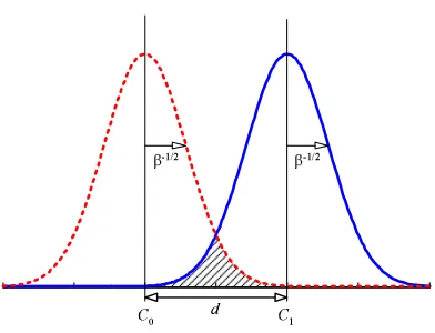
In Section 3.1.1 we saw that optimisation of the proposed noise model and that of Rayleigh’s coef-ficient give equivalent results. In both cases the solution to the discriminant problem was given by adjusting the level ofβ. In order to understand better the physical significance that this represents, it is useful to analyse the problem from the point of view of classification of two populations. Specif-ically, during this section we will refer to the plot in Figure 5 and always assume that both classes have the same cost of misclassification.
In Figure 5, it can be observed that both mapping distributions share the same precision. Under this assumption, for fixed d, we can see that the generalisation error will decrease asβincreases,
i.e. as β−1/2 decreases. From the point of view of projected data, the problem has shifted from computing the direction of discrimination to that of minimising the generalisation error through the adjustment of the variableβ.
The likelihood function L(f)defined in Equation 11 allows us to think ofβas an extra random variable. Hence placing a prior over it not only places a prior over the generalisation error but on
Figure 5: Generalisation error as it relates toβand d. The shaded area gives the generalisation error if the true densities conform to those given by two Gaussians with equal precisionβ. The class centres have been denoted by cqwith q∈ {1,0}.
Rayleigh’s coefficient as well. Consider, for example, the case where d=2 and the class priors are equal: if the data does truly map to the mixture distribution, then the generalisation error will be
Eeq= 1 2−
1 2erf
r
β 2
!
.
Let Equation 11 be a ‘likelihood function’, then by considering a gamma distribution
G
(β|a,b)as a prior,p(β) = b a
Γ(a)β
a−1exp(
−bβ),
the MAP solution forβwill be (see Appendix D)
ˆ
βMAP= N+2a−2 σ2
1+σ20+2b
. (27)
By setting a=b=0.5 we indirectly obtain a uniform distribution over Eeq, which is also a chi-square distribution with one degree of freedom. This special case leads to a new expression of the form
ˆ
βMAP= N−1 σ2
1+σ20+1
, (28)
which can be viewed as a regularised version of Equation 8. The prior could also be used to biasβ towards low or high generalisation errors if this is thought appropriate.
OTHERSPECIALCASES
Taking the limit asβ→0 causes the mean prediction for f? and its variance to take on a much simpler form,
¯
f?=αTβk where
αβ= d∆ˆy ∆ˆyTK∆ˆy,
and
(σ?)2
=k?−kT
∆ˆyT∆ˆy ∆ˆyTK∆ˆyk.
This result is remarkable for the absence of any requirement to invert the kernel matrix, which greatly reduces the computational requirements of this algorithm. In fact, drivingβto zero leads to the well known Parzen windows classifier, sometimes known as probabilistic neural network, (Duda and Hart, 1973). See the work of Schölkopf and Smola (2002) or Roth (2005) for some related studies in limiting cases.
7. Optimising Kernel Parameters
One key advantage of our formulation is that it leads to a principled approach for determining all the model parameters. In the Bayesian formalism it is quite common to make use of the marginal likelihood to reach this purpose, therefore we look to optimise
L
(Θt) =log p(t|D
,Θt),with respect to the model parametersΘt. Recall in Section 3.1 that we optimised the likelihood with
respect to the parameters c0and c1leading to a new encoding of the targets ˆtq=
fTyq Nq
yq.
We back substituted these values into the likelihood in order to demonstrate the equivalence with maximisation of Rayleigh’s coefficient. Unfortunately, one side effect of this process is that it makes the new targets ˆt dependent on the inputs. As a consequence, the targets will shift when-ever the kernel parameters are changed. As expressed in Section 3.1.1, one solution could be to iterate between determining t0, t1and optimising the rest of the parameters. This approach is sim-ple, but it may be difficult to prove convergence properties. We therefore prefer to rely on an expectation-maximisation (EM) algorithm (Dempster et al., 1977) which finesses this issue and for which convergence is proved.
7.1 EM Algorithm
We denote the parameters of the prior as Θk and the complete set of model parameters as Θt = {Θk,β}. Then the goal is to solve the problem arg maxΘtlog p ˆt
X,Θt
, where we have made use again of the modified targets ˆt. In order to solve the problem, a variational lower bound on the marginal log-likelihood is imposed
L
(Θt)≥ Zq(f)logp ˆt
y,f,β
p(f|X,Θk)
where q(f) is a distribution over the latent variables that is independent on the current value Θt.
EM consists of the alternation of the maximisation of
L
with respect to q(f)andΘt, respectively,by holding the other fixed. This procedure repeated iteratively guarantees a local maxima for the marginal likelihood will be found. Thus our algorithm will be composed of the alternation of the following steps:
E-step Given the current parametersΘitt, approximate the posterior with
qit(f)∝exp
−12fTΣ−p1f
,
where
Σp= K−1+βL
−1
. (30)
M-step Fix qit(f)to its current value and make the update Θit+1
t =arg maxΘ
t
L
, (31)where the evidence is computed as
L
=log p ˆty,f,β
p(f|X,Θk)
q(f). We have used the notation
h·ip(x)to indicate an expectation under the distribution p(x).
Maximisation with respect to Θk, the kernel parameters, cannot be done in closed form and
has to rely on some optimisation routine, for example gradient descent, therefore it is necessary to specify the gradients of Equation 29 w.r.t. Θk. An update forβcan be worked out quite easily
because the maximisation of
L
with respect to this parameter has a closed form solution. The expression obtained is of the formˆ
βit = N
¯ σ2
1+σ¯20
,
where ¯σ21=∑yn
D
(fn−µ1)2
E
and the expectationh·iis computed under the predictive distribution
for the nth training point, see Equation 21. An expression for ¯σ20is given in a similar way. 7.2 Updatingβ
Following our discussion in Section 6, we propose (and in fact used) Equation 28 to update the value ofβat every iteration. We repeat the expression here
ˆ βit
MAP=
N−1 ¯ σ2
1+σ¯20+1
. (32)
The resulting optimisation framework is outlined in Algorithm 1.
8. Experiments
Algorithm 1 A possible ordering of the updates. Select Convergence tolerancesηβandηΘk. Set Initial valuesΘ(k0)and ˆβ(0).
Require Data-set
D
= (X,y).while change in ˆβ(it)<ηβand change inΘ(kit)<ηΘk do
• Compute kernel matrix K usingΘ(kit).
• UpdateΣpwith Equation 30
• Use scale conjugate gradients to maximise
L
with respect toΘ(kit). Apply Equation 31• Update ˆβ(it), use Equation 32. end
8.1 Toy Data
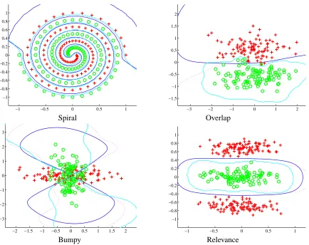
As a first experiment, we compared the KFD, LS-SVM and BFD algorithms on four synthetic data sets using an RBF kernel. Additionally, as a second experiment, we used BFD with an ARD prior on the same data sets to observe some of the capabilities of our approach. In order to facilitate further reference, each data set will be named according to its characteristics. Firstly, Spiral6can only be separated by highly non-linear decision boundaries. Overlap comes from two Gaussian distributions with equal covariance, and is expected to be separated by a linear plane. Bumpy comes from two Gaussians but by being rotated at 90 degrees, quadratic boundaries are called for. Finally, Relevance is a case where only one dimension of the data is relevant to separate the data.
We hypothesized BFD would perform better than LS-SVM and KFD in all the cases because it models directly the class conditional densities. In order to compare the three approaches, we trained KFD, LS-SVM and BFD classifiers with a standard RBF kernel, as specified in Appendix E. Model parameters for KFD and LS-SVM were selected by 10-fold cross-validation whereas BFD was trained by maximising the evidence, using Algorithm 1.
In Figure 6 we present a comparison of the three algorithms. We can observe a similar perfor-mance in the case of Spiral; however it is encouraging to observe that BFD gives more accurate results in the rest of the cases. Despite not producing a straight line, KFD and BFD give accu-rate results in Overlap, whereas LS-SVM overfits. If none of the algorithms sepaaccu-rates this data set with a line it is because obtaining a linear boundary from an RBF kernel is extremely difficult (see Gramacy and Lee, 2005). In Bumpy, the three algorithms give arguably the same solution, with BFD having the smoothest boundary. Lastly, in Relevance all the algorithms provide accurate results, with BFD giving the smoothest solution. In all these experiments we set the initialΘt =1
for BFD and furthermore, observed that BFD did not present any initialisation problems. In all our simulations, we let the algorithm stop wheneverηβ<1×10⁻⁶or the change inηΘk <1×10⁻⁶.
As a second experiment, we were interested in training BFD to test the different facets of the following kernel
k xi,xj=θ1exp
−θ22 xi−xjTΘard xi−xj
+θ3 xiTΘardxj+θ4+θ5δi j, (33)
−1 −0.5 0 0.5 1 −1
−0.8 −0.6 −0.4 −0.2 0 0.2 0.4 0.6 0.8 1
−3 −2 −1 0 1 2 −1.5
−1 −0.5 0 0.5 1 1.5 2
Spiral Overlap
−2 −1.5 −1 −0.5 0 0.5 1 1.5 2 −3
−2 −1 0 1 2 3
−1 −0.5 0 0.5 1 −1
−0.8 −0.6 −0.4 −0.2 0 0.2 0.4 0.6 0.8 1
Bumpy Relevance
Figure 6: Comparison of classification of synthetic data sets using an RBF kernel. Two classes are shown as pluses and circles. The separating lines were obtained by projecting test data over a grid. The lines in blue (dark), magenta (dashed) and cyan (gray) were obtained with BFD, KFD and LS-SVM respectively. Kernel and regularisation parameters for KFD and LS-SVM were obtained by 10-fold cross validation, whereas BFD related parameters were obtained by evidence maximisation. We trained BFD using Algorithm 1; details of our implementations are given in Appendix E.
whereδi j is the Kronecker delta and the matrixΘard =diag(θ6, . . . ,θ6+d−1)with d being the di-mension of X. This kernel has four components: an RBF part composed of(θ1,θ2,Θard); a linear
part, composed of (θ3,Θard); a bias term given by θ4 and the so-called ‘nugget’ termθ5 which,
for a large enough valueθ5, ensures that K is positive definite and therefore invertible at all times. Therefore, the parameters of the model areΘt = (Θk,β), withΘk= (θ1, . . . ,θ6+d−1).
On this occassion, BFD got stuck into local minima so we resorted to do model selection to choose the best solution. This process was carried out by training each data set with three different initial values forθ2while the remainingθi6=2were always initialised to 1. In the cases of Bumpy and Relevance we made the initialθ2=
10−2,10−1,1
stop whenever ηβ <1×10⁻⁶ or the change in ηΘk <1×10−
6. The parameter β was always initialised to 1. The selected models for each set are summarised in Figure 7.
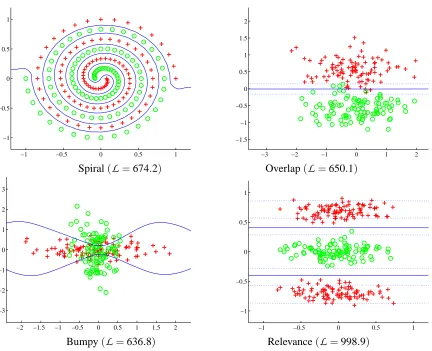
The results are promising. In Spiral, the separating plane is highly non-linear as expected. Meanwhile, we observe in Overlap that the predominating decision boundary in the solution is linear. In Bumpy, the boundary starts to resemble a quadratic and, finally, for Relevance, only one dimension of the data is used to classify the data. Note that the values forΘk, summarised in Table 1,
go in accordance with these observations. For example, in Overlap and Relevance, the value of θ6is significantly lower thanθ7, indicating that only one dimension of the data is relevant for the solution. This is markedly different to the cases of Spiral and Bumpy, where both dimensions (θ6 andθ7) have been given relatively the same weights. Hence, for every case we have obtained sensible solutions. All the kernel parameters determined by the algorithm, for the four experiments, are given in Table 1.
−1 −0.5 0 0.5 1 −1
−0.5 0 0.5 1
−3 −2 −1 0 1 2 −1.5
−1 −0.5 0 0.5 1 1.5 2
Spiral(
L
=674.2) Overlap(L
=650.1)−2 −1.5 −1 −0.5 0 0.5 1 1.5 2 −3
−2 −1 0 1 2 3
−1 −0.5 0 0.5 1 −1
−0.5 0 0.5 1
Bumpy(
L
=636.8) Relevance(L
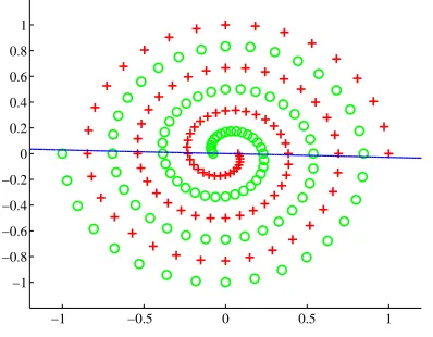
=998.9)Figure 8 shows an example of the result of training Spiral with a poor initialisation. It can be seen that the value of the marginal likelihood in this case is smaller to the one presented in Figure 7. However, this behaviour is not exclusive of BFD, indeed we observed a very similar situation with a poorly initialised Bayesian LS-SVM and with KFD cross-validated with a badly selected grid.
−1 −0.5 0 0.5 1 −1
−0.8 −0.6 −0.4 −0.2 0 0.2 0.4 0.6 0.8 1
Figure 8: The solution for the spiral data with a poor initialisationθ2=1. Associated log-likelihoodL=
562.7.
Experiment lnθ1 lnθ2 lnθ3 lnθ4 lnθ5 lnθ6 lnθ7 Spiral 8.5015 −9.5588 1.0139 −4.9759 −10.6373 −2.78 −2.9609 Overlap 0.5011 −7.9801 1.1455 −4.8319 −8.5990 −6.9953 −0.1026 Bumpy 4.9836 −10.8222 1.1660 −4.7495 −13.5996 −3.9131 −3.7030 Relevance 4.6004 −9.5036 1.2734 −4.9351 −13.8155 −6.9968 −1.5386
Table 1: log-values of the parameters learnt with BFD for the different toy experiments. In Overlap and
Relevance, the weights of the featureθ6are low if compared with the featureθ7. This is in contrast
with Spiral and Bumpy, where both features have been given relatively the same weights.
8.2 Benchmark Data Sets
In order to evaluate the performance of our approach, we tested five different algorithms on well known problems. The algorithms used were: linear and quadratic discriminants (LDA and QDA), KFD, LS-SVM and BFD. The last two algorithms provided the opportunity to use ARD priors so they were reported as well. We used a synthetic set (banana) along with 12 other real world data sets coming from the UCI, DELVE and STATLOG repositories.7 In particular, we used instances of these data that had been preprocessed an organised by Rätsch et al. (1998) to do binary classification tests. The main difference between the original data and Rätsch’s is that he converted every problem
into binary classes and randomly partitioned every data set into 100 training and testing instances.8 In addition, every instance was normalised to have zero mean and unit standard deviation. More details can be found at (Rätsch et al., 1998).
Mika et al. (1999) and Van Gestel et al. (2002) have given two of the most in depth comparisons of algorithms related to FLD. Unfortunately, the reported performance in both cases is given in terms of test-set accuracy (or error rates), which implied not only the adjustment of the bias term but also the implicit assumption that the misclassification costs of each class were known. Given that discriminant methods operate independently of the method of bias choice, we felt it more appropriate to use a bias independent measure like the area under the ROC curve (AUC).
The LDA and QDA classifiers were provided by the Matlab functionclassifywith the options ‘linear’ and ‘quadratic’, respectively. In both cases, no training phase was required, as described by Michie et al. (1994). The output probabilities were used as latent values to trace the curves. Meanwhile, for KFD’s parameter selection we made use of the parameters obtained previously by Mika et al. (1999) and which are available at http://mlg.anu.edu.au/˜raetsch. The ROC curves for KFD were thus generated by projecting every instance of the test set over the direction of discrimination.
Mika trained a KFD on the first five training partitions of a given data set and selected the model parameters to be the median over those five estimates. A detailed explanation of the experimental setup for KFD and related approaches can be found in Rätsch et al. (1998) and Mika et al. (1999). In the case of LS-SVM, we tried to follow a similar process to estimate the parameters, hence we trained LS-SVM’s on the first five realisations of the training data and then selected the median of the resulting parameters as estimates. In the same way, projections of test data were used to generate the ROC curves.
Finally, for BFD we also tried to follow the same procedure. We trained a BFD model with Nx=8
different initialisations over the first five training instances of each data set. Hence we obtained an array of parameters of dimensions 8×5 where the rows were the initialisations, the columns were the partitions and each element a vectorΘt. For each column, we selected the results that gave the
highest marginal likelihood, so that the array reduced from 40 to only 5 elements. Then we followed the KFD procedure of selecting the median over those parameters. In these experiments, we used the tolerancesηβandηΘk to be less than 1×10⁻⁶. More details of the experimental setup are given in Appendix E.
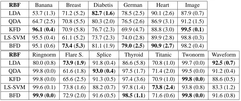
In Table 2 we report the averages of the AUC’s over all the testing instances of a given data set. In the cases of KFD, LS-SVM and BFD we used the RBF kernel of Appendix E. Computation of the ROC curves were done with the functionROCprovided by Pelckmans et al. (2003) and Suykens et al. (2002) and no further processing of the curves was required, for instance removing convexities was unnecessary.
It can be observed that BFD outperforms all the other methods in 613 data sets, comes second in 3 cases and third in the remaining 4. In particular, it is remarkable to see BFD performing consistently better than KFD across most of the problem domains. It seems that leaving the ‘regression to the labels’ assumption pays-off in terms of areas under the ROC curves. It is also interesting to observe that LDA performs well in almost all the problems (except banana) and it thus indicates that most of these data sets could be separated with a linear hyperplane with acceptable results. From these results we can conclude that the better designed noise model in BFD allows it to outperform ‘similar’