A Classification Framework for Anomaly Detection

A Classification Framework for Anomaly Detection

Ingo Steinwart [email protected]

Don Hush [email protected]

Clint Scovel [email protected]

Modeling, Algorithms and Informatics Group, CCS-3 Los Alamos National Laboratory

Los Alamos, NM 87545, USA

Editor: Bernhard Sch¨olkopf

Abstract

One way to describe anomalies is by saying that anomalies are not concentrated. This leads to the problem of finding level sets for the data generating density. We interpret this learning problem as a binary classification problem and compare the corresponding classification risk with the standard performance measure for the density level problem. In particular it turns out that the empirical classification risk can serve as an empirical performance measure for the anomaly detection prob-lem. This allows us to compare different anomaly detection algorithms empirically, i.e. with the help of a test set. Furthermore, by the above interpretation we can give a strong justification for the well-known heuristic of artificially sampling “labeled” samples, provided that the sampling plan is well chosen. In particular this enables us to propose a support vector machine (SVM) for anomaly detection for which we can easily establish universal consistency. Finally, we report some experi-ments which compare our SVM to other commonly used methods including the standard one-class SVM.

Keywords: unsupervised learning, anomaly detection, density levels, classification, SVMs

1. Introduction

Anomaly (or novelty) detection aims to detect anomalous observations from a system. In the ma-chine learning version of this problem we cannot directly model the normal behaviour of the system since it is either unknown or too complex. Instead, we have some sample observations from which the normal behaviour is to be learned. This anomaly detection learning problem has many important applications including the detection of e.g. anomalous jet engine vibrations (see Nairac et al., 1999; Hayton et al., 2001; King et al., 2002), abnormalities in medical data (see Tarassenko et al., 1995; Campbell and Bennett, 2001), unexpected conditions in engineering (see Desforges et al., 1998) and network intrusions (see Manikopoulos and Papavassiliou, 2002; Yeung and Chow, 2002; Fan et al., 2001). For more information on these and other areas of applications as well as many methods for solving the corresponding learning problems we refer to the recent survey of Markou and Singh (2003a,b).

Sch¨olkopf and Smola, 2002). To make this precise let Q be our unknown data-generating distribu-tion on the input space X which has a density h with respect to a known reference distribudistribu-tion µ on X . Obviously, the density level sets{h>ρ},ρ>0, describe the concentration of Q. Therefore to

define anomalies in terms of the concentration one only has to fix a threshold levelρ>0 so that a

sample x∈X is considered to be anomalous whenever h(x)≤ρ. Consequently, our aim is to find

the set{h≤ρ}to detect anomalous observations, or equivalently, theρ-level set{h>ρ}to describe normal observations.

We emphasize that given the data-generating distribution Q the choice of µ determines the

den-sity h, and consequently anomalies are actually modeled by both µ andρ. Unfortunately, many

pop-ular algorithms are based on density estimation methods that implicitly assume µ to be the uniform distribution (e.g. Gaussian mixtures, Parzen windows and k-nearest neighbors density estimates)

and therefore for these algorithms defining anomalies is restricted to the choice ofρ. With the lack

of any further knowledge one might feel that the uniform distribution is a reasonable choice for µ, however there are situations in which a different µ is more appropriate. In particular, this is true if we consider a modification of the anomaly detection problem where µ is not known but can be sampled from. We will see that unlike many others our proposed method can handle both problems. Finding level sets of an unknown density is also a well known problem in statistics which has some important applications different from anomaly detection. For example, it can be used for the problem of cluster analysis as described in by Hartigan (1975) and Cuevas et al. (2001), and for testing of multimodality (see e.g. M¨uller and Sawitzki, 1991; Sawitzki, 1996). Some other appli-cations including estimation of non-linear functionals of densities, density estimation, regression analysis and spectral analysis are briefly described by Polonik (1995). Unfortunately, the algo-rithms considered in these articles cannot be used for the anomaly detection problem since the imposed assumptions on h are often tailored to the above applications and are in general unrealistic for anomalies.

One of the main problems of anomaly detection—or more precisely density level detection—is the lack of an empirical performance measure which allows us to compare the generalization perfor-mance of different algorithms by test samples. By interpreting the density level detection problem as binary classification with respect to an appropriate measure, we show that the corresponding empir-ical classification risk can serve as such an empirempir-ical performance measure for anomaly detection. Furthermore, we compare the excess classification risk with the standard performance measure for the density level detection problem. In particular, we show that both quantities are asymptotically equivalent and that simple inequalities between them are possible under mild conditions on the density h.

2. Detecting Density Levels is a Classification Problem

We begin with rigorously defining the density level detection (DLD) problem. To this end let(X,

A

)

be a measurable space and µ a known distribution on(X,

A

). Furthermore, let Q be an unknown

distribution on(X,

A

)which has an unknown density h with respect to µ, i.e. dQ=hdµ. Given a

ρ>0 the set{h>ρ}is called theρ-level set of the density h. Throughout this work we assume that

{h=ρ}is a µ-zero set and hence it is also a Q-zero set. For the density level detection problem and

related tasks this is a common assumption (see e.g. Polonik, 1995; Tsybakov, 1997).

Now, the goal of the DLD problem is to find an estimate of the ρ-level set of h. To this end

we need some information which in our case is given to us by a training set T = (x1, . . . ,xn)∈

Xn. We will assume in the following that T is i.i.d. drawn from Q. With the help of T a DLD

algorithm constructs a function fT: X →Rfor which the set{fT>0}is an estimate of theρ-level

set{h>ρ}of interest. Since in general{fT>0}does not excactly coincide with{h>ρ}we need

a performance measure which describes how well{fT>0}approximates the set{h>ρ}. Probably

the best known performance measure (see e.g. Tsybakov, 1997; Ben-David and Lindenbaum, 1997,

and the references therein) for measurable functions f : X→Ris

S

_µ,h,ρ(f) := µ

{f>0}M_{h>ρ_}

,

whereM_{denotes the symmetric difference. Obviously, the smaller}

S

_µ,h,ρ(f)is, the more{f >0}

coincides with theρ-level set of h and a function f minimizes

S

µ,h,ρif and only if{f>0}is µ-almost surely identical to{h>ρ}. Furthermore, for a sequence of functions fn: X→Rwith

S

µ,h,ρ(fn)→0

we easily see that sign fn(x)→1{h>ρ}(x)for µ-almost all x∈X , and since Q is absolutely continuous

with respect to µ the same convergence holds Q-almost surely. Finally, it is important to note, that the performance measure

S

_µ,h,ρis insensitive to µ-zero sets. Since we cannot detect µ-zero sets using

a training set T drawn from Qnthis feature is somehow natural for our model.

Although

S

_µ,h,ρseems to be well-adapted to our model, it has a crucial disadvantage in that we

cannot compute

S

_µ,h,ρ(f) since{h>ρ} is unknown to us. Therefore, we have to estimate it. In

our model the only information we can use for such an estimation is a test set W = (x1, . . . ,ˆ xˆm)

which is i.i.d. drawn from Q. Unfortunately, there is no method known to estimate

S

µ,h,ρ(f)from

W with guaranteed accuracy in terms of m, f , µ andρ, and we strongly believe that such a method cannot exist. Because of this lack, we cannot empirically compare different algorithms in terms of the performance measure

S

µ,h,ρ.

Let us now describe another performance measure which has merits similar to

S

_µ,h,ρbut

addi-tionally has an empirical counterpart, i.e. a method to estimate its value with guaranteed accuracy by only using a test set. This performance measure is based on interpreting the DLD problem as a binary classification problem in which T is assumed to be positively labeled and infinitely many negatively labeled samples are available by the knowledge of µ. To make this precise we write

Y :={−1,1}and define

Definition 1 Let µ and Q be probability measures on X and s∈(0,1). Then the probability measure Q sµ on X×Y is defined by

Q sµ(A) := sEx∼Q1A(x,1) + (1−s)Ex∼µ1A(x,−1)

Roughly speaking, the distribution Q sµ measures the “1-slice” of A⊂X×Y by sQ and the

“−1-slice” by (1−s)µ. Moreover, the measure P :=Q sµ can obviously be associated with a

binary classification problem in which positive samples are drawn from sQ and negative samples

are drawn from(1−s)µ. Inspired by this interpretation let us recall that the binary classification

risk for a measurable function f : X→Rand a distribution P on X×Y is defined by

R

_P(f) = P {(x,y): sign f(x)6=y}

,

where we define signt :=1 if t>0 and signt=−1 otherwise. Furthermore, the Bayes risk

R

_Pof P

is the smallest possible classification risk with respect to P, i.e.

R

_P := inf

n

R

_P(f)

f : X→Rmeasurable o

.

We will show in the following that learning with respect to

S

µ,h,ρ is equivalent to learning with

respect to

R

_P(.). To this end we begin by computing the marginal distribution PX and the supervisor

η(x):=P(y=1|x), x∈X , of P :=Q sµ:

Proposition 2 Let µ and Q be probability measures on X such that Q has a density h with respect to µ, and let s∈(0,1). Then the marginal distribution of P :=Q sµ on X is PX =sQ+ (1−s)µ.

Furthermore, we PX-a.s. have

P(y=1|x) = sh(x)

sh(x) +1−s.

Proof As recalled in the appendix, P(y=1|x), x∈X , is a regular conditional probability and hence we only have to check the condition of Corollary 19. To this end we first observe by the definition

of P :=Q sµ that for all non-negative, measurable functions f : X×Y →Rwe have

Z

X×Y f dP = s Z

X

f(x,1)Q(dx) + (1−s)

Z

X

f(x,−1)µ(dx).

Therefore, for A∈

A

we obtain

Z

A×Y

sh(x)

sh(x) +1−sP(dx,dy)

= s

Z

A

sh(x)

sh(x) +1−sh(x)µ(dx) + (1−s)

Z

A

sh(x)

sh(x) +1−sµ(dx)

=

Z

A

sh(x)µ(dx)

= s

Z

A

1_X×{1}(x,1)Q(dx) + (1−s)

Z

A

1_X×{1}(x,−1)µ(dx) =

Z

A×Y1X×{1}dP.

Note that the formula for the marginal distribution PX in particular shows that the µ-zero sets

of X are exactly the PX-zero sets of X . As an immediate consequence of the above proposition we

additionally obtain the following corollary which describes theρ-level set of h with the help of the

Corollary 3 Let µ and Q be probability measures on X such that Q has a density h with respect to µ. Forρ>0 we write s :=_1+ρ1 and define P :=Q sµ. Then forη(x):=P(y=1|x), x∈X , we have

µ{η>1/2}M{_h>ρ}

= 0,

i.e.{η>1/2}µ-almost surely coincides with{h>ρ}.

Proof By Proposition 2 we see thatη(x)>1₂ is µ-almost surely equivalent to _sh(sh_x)+1(x)_−s >1₂ which is equivalent to h(x)>1−s_s =ρ.

The above results in particular show that every distribution P :=Q sµ with dQ :=hdµ and

s∈(0,1) determines a triple (µ,h,ρ) with ρ:= (1−s)/s and vice-versa. In the following we

therefore use the shorthand

S

_P(f):=

S

_µ,h,ρ(f).

Let us now compare

R

P(.) with

S

P(.). To this end recall, that binary classification aims to

discriminate{η>1/2}from{η<1/2}. In view of the above corollary it is hence no surprise that

R

_P(.)can serve as a surrogate for

S

_P(.)as the following theorem shows:

Theorem 4 Let µ and Q be probability measures on X such that Q has a density h with respect to µ. Letρ>0 be a real number which satisfies µ({h=ρ}) =0. We write s := 1

1+ρ and define P :=Q sµ. Then for all sequences (fn) of measurable functions fn: X →R the following are

equivalent:

i)

S

P(fn)→0.

ii)

R

_P(fn)→

R

P.

In particular, for a measurable function f : X→Rwe have

S

_P(f) =0 if and only if

R

_P(f) =

R

_P.

Proof For n∈Nwe define En:={fn>0}M{h>ρ}. Since by Corollary 3 we know µ({h>ρ}M

{η>1

2}) =0 it is easy to see that the classification risk of fncan be computed by

R

_P(fn) =

R

P+ Z

En

|2η−1|dPX. (1)

Now, {|2η−1|=0}is a µ-zero set and hence a PX-zero set. The latter implies that the measures

|2η−1|dPX and PX are absolutely continuous with respect to each other, and hence we have

|2η−1|dPX(En)→0 if and only if PX(En)→0.

Furthermore, we have already observed after Proposition 2 that PX and µ are absolutely continuous

with respect to each other, i.e. we also have

PX(En)→0 if and only if µ(En)→0.

Therefore, the assertion follows from

S

_P(fn) =µ(En).

Theorem 4 shows that instead of using

S

P as a performance measure for the density level

de-tection problem one can alternatively use the classification risk

R

_P(.). Therefore, we will

Proposition 5 Let µ and Q be probability measures on X . Forρ>0 we write s := 1

1+ρ and define P :=Q sµ. Then for all measurable f : X→Rwe have

R

_P(f) = 1

1+ρEQI(1,sign f) +

ρ

1+ρEµI(−1,sign f).

Furthermore, for the Bayes risk we have

R

_P ≤ min

n 1

1+ρ,

ρ

1+ρ

o

and

R

_P = 1

1+ρEQ1{h≤ρ}+

ρ

1+ρEµ1{h>ρ}.

Proof The first assertion directly follows from

R

P(f) = P {(x,y): sign f(x)6=y}

= P {(x,1): sign f(x) =−1}

+P {(x,−1): sign f(x) =1}

= sQ {sign f =−1}

+ (1−s)µ {sign f =1}

= sE_QI(1,sign f) + (1−s)E_µI(−1,sign f).

The second assertion directly follows from

R

P≤

R

P(1X)≤s and

R

P≤

R

P(−1X)≤1−s. Finally,

for the third assertion recall that f =1_{h>ρ}−1_{h≤ρ}is a function which realizes the Bayes risk.

As described at the beginning of this section our main goal is to find a performance measure for the density level detection problem which has an empirical counterpart. In view of Proposition 5 the choice of an empirical counterpart for

R

_P(.)is rather obvious:

Definition 6 Let µ be a probability measure on X andρ>0. Then for T= (x1, . . . ,xn)∈Xnand a

measurable function f : X→Rwe define

R

_T(f) := 1 (1+ρ)n

n

∑

i=1

I(1,sign f(xi)) +

ρ

1+ρEµI(−1,sign f).

If we identify T with the corresponding empirical measure it is easy to see that

R

_T(f) is the

classification risk with respect to the measure T sµ for s := _1+ρ1 . Then for measurable functions

f : X →R, e.g. Hoeffding’s inequality shows that

R

T(f)approximates the true classification risk

R

_P(f)in a fast and controllable way.

It is highly interesting that the classification risk

R

_P(.)is strongly connected with another

ap-proach for the density level detection problem which is based on the so-called excess mass (see e.g. Hartigan, 1987; M¨uller and Sawitzki, 1991; Polonik, 1995; Tsybakov, 1997, and the refer-ences therein). To be more precise let us first recall that the excess mass of a measurable function

f : X→Ris defined by

E

_P(f) := Q({f >0})−ρµ({f >0}),

where Q,ρand µ have the usual meaning. The following proposition shows that

R

P(.)and

E

P(.)

Proposition 7 Let µ and Q be probability measures on X . Forρ>0 we write s := 1

1+ρ and define P :=Q sµ. Then for all measurable f : X→Rwe have

E

_P(f) = 1−(1+ρ)

R

_P(f).

Proof We obtain the assertion by the following simple calculation:

E

P(f) = Q({f>0})−ρµ({f≥0})

= 1−Q({f ≤0})−ρµ({f >0})

= 1−Q {sign f =−1}

−ρµ {sign f =1}

= 1−(1+ρ)

R

_P(f).

If Q is an empirical measure based on a training set T in the definition of

E

P(.)then we obtain

am empirical performance measure which we denote by

E

_T(.). By the above proposition we have

E

_T(f) =1−1

n

n

∑

i=1

I(1,sign f(xi))−ρEµI(−1,sign f) =1−(1+ρ)

R

T(f) (2)

for all measurable f : X →R. Now, given a class

F

of measurable functions from X to R the

(empirical) excess mass approach considered e.g. by Hartigan (1987); M¨uller and Sawitzki (1991);

Polonik (1995); Tsybakov (1997), chooses a function fT ∈

F

which maximizes

E

T(.)within

F

.

By equation (2) we see that this approach is actually a type of empirical risk minimization (ERM). Surprisingly, this connection has not been observed, yet. In particular, the excess mass has only been considered as an algorithmic tool, but not as a performance measure. Instead, the papers dealing

with the excess mass approach measures the performance by

S

P(.). In their analysis an additional

assumption on the behaviour of h around the levelρis required. Since this condition can also be

used to establish a quantified version of Theorem 4 we will recall it now:

Definition 8 Let µ be a distribution on X and h : X→[0,∞)be a measurable function withR

hdµ=

1, i.e. h is a density with respect to µ. Forρ>0 and 0≤q≤∞we say that h hasρ-exponent q if

there exists a constant C>0 such that for all sufficiently small t>0 we have

µ {|h−ρ| ≤t}

≤ Ctq. (3)

Condition (3) was first considered by Polonik (1995, Thm. 3.6). This paper also provides an

example of a class of densities onRd, d≥2, which has exponent q=1. Later, Tsybakov (1997,

p. 956) used (3) for the analysis of a density level detection method which is based on a localized version of the empirical excess mass approach.

Interestingly, condition (3) is closely related to a concept for binary classification called the Tsybakov noise exponent (see e.g. Mammen and Tsybakov, 1999; Tsybakov, 2004; Steinwart and Scovel, 2004) as the following proposition proved in the appendix shows:

Proposition 9 Let µ and Q be distributions on X such that Q has a density h with respect to µ. For

i) h hasρ-exponent q.

ii) P has Tsybakov noise exponent q, i.e. there exists a constant C>0 such that for all sufficiently small t>0 we have

PX |2η−1| ≤t

≤ C·tq (4)

In recent years Tsybakov’s noise exponent has played a crucial role for establishing learning

rates faster than n−12 for certain algorithms (see e.g. Mammen and Tsybakov, 1999; Tsybakov, 2004;

Steinwart and Scovel, 2004). Remarkably, it was already observed by Mammen and Tsybakov (1999), that the classification problem can be analyzed by methods originally developed for the DLD problem. However, to our best knowledge the exact relation between the DLD problem and binary classification has not been presented, yet. In particular, it has not been observed yet, that this relation opens a non-heuristic way to use classification methods for the DLD problem as we will discuss in the next section.

As already announced we can also establish inequalities between

S

Pand

R

P(.)with the help of

theρ-exponent. This is done in the following theorem:

Theorem 10 Letρ>0 and µ and Q be probability measures on X such that Q has a density h with respect to µ. For s := 1

1+ρwe write P :=Q sµ. Then the following statements hold:

i) If h is bounded then there exists a constant c>0 such that for all measurable f : X→Rwe have

R

_P(f)−

R

_P ≤ c

S

_P(f).

ii) If h hasρ-exponent q∈(0,∞]then there exists a constant c>0 such that for all measurable f : X→Rwe have

S

P(f) ≤ c

R

P(f)−

R

P ₁₊q_q

.

Proof The first assertion directly follows from (1) and Proposition 2. The second assertion follows from Proposition 9 and a result of Tsybakov (2004, Prop. 1).

Remark 11 We note that many of the results of this section can be generalized to the case where Q is not absolutely continuous with respect to µ. Indeed, select an auxilliary measureνsuch that both Q and µ are absolutely continuous with respect to ν. For example one could choose ν=

Q+µ

2 . Consequently we have Q=h1νand µ=h2νfor some real valued functions h1 and h2. Then Proposition 2 holds with h(x):=h1(x)

h2(x), where one defines the righthand side to be 0 when h1(x) =

h2(x) =0. One can also show that h is PX-a.s. independent of the choice ofν. Corollary 3 holds

where the measure of the symmetric difference is evaluated with either Q or µ. However it appears that only the “

R

_P(fn)→

R

P⇒

S

P(fn)→0” assertion of Theorem 4 holds instead of equivalence.

3. A Support Vector Machine for Density Level Detection

In the previous section we have shown that the DLD problem can be interpreted as a binary clas-sification problem in which one conditional class probability is known. We now show that this interpretation has far reaching algorithmic consequences. To this end let us assume that we give

each sample of our training set T = (x1, . . . ,xn) drawn from Q the label 1. Additionally we

gen-erate a second training set T0 = (x0₁, . . . ,x0_n0)from µ and label each sample of it with−1. Merging these labeled sample sets gives a new training set which then can be used by a binary classifica-tion algorithm. By our consideraclassifica-tions in the previous secclassifica-tion it seems reasonable to expect that the used classification algorithm actually learns the DLD problem provided that the algorithm is

well-adjusted to the sample set sizes and the parameterρ.

In the following we work this high-level approach out by constructing an SVM for the DLD

problem. To this end let k : X×X→Rbe a positive definite kernel with reproducing kernel Hilbert

space (RKHS) H. Furthermore, let µ be a known probability measure on X and l : Y×R→[0,∞)

be the hinge loss function, i.e. l(y,t):=max{0,1−yt}, y∈Y , t ∈R. Then for a training set

T = (x1, . . . ,xn)∈Xn, a regularization parameterλ>0, andρ>0 we initially define

fT,µ,λ := arg min

f∈Hλkfk

2

H+

1

(1+ρ)n

n

∑

i=1

l(1,f(xi)) +

ρ

1+ρEx∼µl(−1,f(x)), (5)

and

(f˜T,µ,λ,˜bT,µ,λ) := arg min

f∈H b∈R

λkfk2_H+ 1 (1+ρ)n

n

∑

i=1

l(1,f(xi) +b) +

ρ

1+ρEx∼µl(−1,f(x) +b). (6)

The decision function of the SVM without offset is f_T,µ,λ: X→Rand analogously, the SVM with

offset has the decision function ˜fT,µ,λ+˜bT,µ,λ: X →R.

Although the measure µ is known, almost always the expectation E_x∼µl(−1,f(x)) can only

be numerically computed which requires finitely many function evaluations of f . If the integrand of this expectation was smooth we could use some known deterministic methods to choose these function evaluations efficiently. However, since the hinge loss is not differentiable there is no such method known to us. According to our above plan we will therefore use points T0:= (x0₁, . . . ,x0

n0)

which are randomly sampled from µ to approximateE_x∼µl(−1,f(x))by _n10∑n

0

i=1l(−1,f(x0i)). We

denote the corresponding approximate solutions of (5) and (6) by fT,T0_,λ and(f˜_T,T0_,λ,˜b_T,T0_,λ), re-spectively. Furthermore, in these cases the formulations (5) and (6) are identical to the standard L1-SVM formulations besides the weighting factors in front of the empirical error terms. There-fore, the derivation of the corresponding dual problems is straightforward. For example, the dual problem for (6) can be written as follows:

max

n

∑

i=1 αi+

n0

∑

i=1 α0

i−12

n

∑

i,j=1

αiαjk(xi,xj)−1₂ n0

∑

i,j=1 α0

iα0jk(xi0,x0j) + n,n0

∑

i,j=1

αiα0jk(xi,x0j)

s.t. ∑n

i=1αi

− n

0

∑

i=1α

0 i =0,

0≤ αi ≤ _λ(1+ρ)2 _n, i=1, ...,n,

0≤ α0

i ≤ λ(1+ρ)2ρ n0, i=1, ...,n0.

The fact that the SVM for DLD essentially coincides with the standard L1-SVM also allows us to modify many known results for these algorithms. For simplicity we will only state a consistency

result which describes the case where we use n0=n random samples from µ in order to approximate

the expectation with respect to µ. However, it is straight forward to extend the result to the more

general case of n0=rn samples for some positive r∈Q. In order to formulate the result we have to

recall the notion of universal kernels (see Steinwart, 2001). To this end let X be a compact metric

space, say a closed and bounded subset ofRd_{. We denote the space of all continuous functions on}

X by C(X). As usual, this space is equipped with the supremum normk.k_∞. Then the RKHS H of a

continuous kernel k on X is embedded into C(X), i.e. H⊂C(X), where the inclusion is continuous.

We say that the kernel k is universal, if in addition H is dense in C(X), i.e. for every f ∈C(X)and

everyε>0 there exists a g∈H withkf−gk_∞<ε. Some examples of universal kernels including

the Gaussian RBF kernels were presented by Steinwart (2001). Now we can formulate the announced result:

Theorem 12 (Universal consistency) Let X be a compact metric space and k be a universal kernel on X . Furthermore, letρ>0, and µ and Q be probability measures on X such that Q has a density h with respect to µ. For s := _1+ρ1 we write P :=Q sµ. Then for all sequences(λn) of positive

numbers withλn→0 and nλ2n→∞and for allε>0 we have

(Q⊗µ)n(T,T0)∈Xn×Xn:

R

P(fT,T0_,λ

n)≤

R

P+ε

→0,

for n→∞. The same result holds for the SVM with offset if one replaces the condition nλ2_n→∞

by the slightly stronger assumption nλ2_n/log n→∞. Finally, for both SVMs it suffices to assume nλ1+δ_n →∞for someδ>0 if one uses a Gaussian RBF kernel.

Sketch of the Proof Let us introduce the shorthandν=Q⊗µ for the product measure of Q and µ.

Moreover, for a measurable function f : X→Rwe define the function lf : X×X→Rby

lf(x,x0):= 1

1+ρl(1,f(x)) +

ρ

1+ρl(−1,f(x

0_{)), x,x}0_∈X.

Furthermore, we write l◦f(x,y):=l(y,f(x)), x∈X , y∈Y . Then it is easy to check that we always haveE_νlf=E_Pl◦f . Analogously, we seeE_T⊗T0lf=E_T

sT0l◦f , if T⊗T

0_{denotes the product}

measure of the empirical measures based on T and T0. Now, using Hoeffding’s inequality forνit is

easy to establish a concentration inequality in the sense of Steinwart (2005, Lem. III.5). The rest of the proof is analogous to the steps of Steinwart (2005).

Recall that by Theorem 4 consistency with respect to

R

_P(.) is equivalent to consistency with

respect to

S

P(.). Therefore we immediately obtain the following corollary

Corollary 13 Under the assumptions of Theorem 12 both the DLD-SVM with offset and without offset are universally consistent with respect to

S

P(.), i.e.

S

P(f˜T,µ,λ+˜bT,µ,λ)→0 and

S

P(fT,T0_,λ

n)→0

in probability.

a similar approach and analysis is possible for many other classification algorithms. This gives a strong justification for the well-known heuristic of adding artificial samples to anomaly detection problems with unlabeled data. However, it is important to note that this justification only holds for the above sampling plan and suitably adjusted classification algorithms, and that other, heuristic sample plans may actually lead to bad learning performance (cf. the second part of Section 5)

4. Experiments

We present experimental results for anomaly detection problems where the set X is a subset ofRd_.

A total of four different learning algorithms are used to produce functions f which declare the set

{x : f(x)≤0}anomalous. A distinct advantage of the formulation in Section 2 is that it allows us

to make quantitative comparisons of different functions by comparing estimates of their risk

R

P(f)

which can be computed from sample data. In particular consider a data set pair (S,S0) where S

contains samples drawn from Q and S0 contains samples drawn from µ (in what follows(S,S0_)is

either training data, validation data, or test data). Based on Definition 6 we define the empirical risk of f with respect to(S,S0)to be

R

_(S,S0₎(f) = 1

(1+ρ)|S|_x∈S

∑

I(1,sign f(x)) +

ρ

(1+ρ)|S0_|

∑

x∈S0

I(−1,sign f(x)). (8)

A smaller risk indicates a better solution to the DLD problem. Since the risk

R

P(·)depends

ex-plicitly onρadditional insight into the performance of f can be obtained from the two error terms.

Specifically the quantity _|S|1 ∑_x∈SI(1,sign f(x)) is an estimate of Q({f ≤0}) which we call the alarm rate (i.e. the rate at which samples will be labeled anomalous by f ), and the quantity

1

|S0_|∑x∈S0I(−1,sign f(x)) is an estimate of µ({f >0}) which we call the volume of the predicted normal set. There is an obvious trade-off between these two quantities, i.e. for the optimal

solu-tions for fixedρsmaller alarm rates correspond to larger volumes and vice versa. Also, from the

expression for the risk in Proposition 5 it is clear that for any two functions with the same alarm rate we prefer the function with the smaller volume and vice versa. More generally, when comparing different solution methods it is useful to consider the values of these quantities that are achieved

by varying the value of ρ in the design process. Such performance curves are presented in the

comparisons below.

We consider three different anomaly detection problems, two are synthetic and one is an applica-tion in cybersecurity. In each case we define a problem instance to be a triplet consisting of samples

from Q, samples from µ, and a value for the density levelρ. We compare four learning algorithms

that accept a problem instance and automatically produce a function f : the density level detec-tion support vector machine (DLD–SVM), the one-class support vector machine (1CLASS–SVM), the Gaussian maximum-likelihood (GML) method, the mixture of Gaussians maximum-likelihood

(MGML) method.1 The first is the algorithm introduced in this paper, the second is an algorithm

based on the the one-class support vector machine introduced by Sch¨olkopf et al. (2001) and the others (including the Parzen windows method) are based on some of the most common

paramet-ric and non-parametparamet-ric statistical methods for density-based anomaly detection inRd. Each of the

four learning algorithms is built on a core procedure that contains one or more free parameters. The availability of a computable risk estimate makes it possible to determine values for these parameters

using a principled approach that is applied uniformly to all four core procedures. In particular this is accomplished as follows in our experiments. The data in each problem instance is partitioned into three pairs of sets; the training sets(T,T0), the validation sets(V,V0)and the test sets(W,W0). The core procedures are run on the training sets and the values of the free parameters are chosen to min-imize the empirical risk (8) on the validation sets. The test sets are used to estimate performance. We now describe the four learning algorithms in detail.

In the DLD–SVM algorithm we employ the SVM with offset described in Section 3 with a Gaussian RBF kernel

k(x,x0) =e−σ2kx−x0k2.

Withλandσ2_{fixed and the expected valueE}

x∼µl(−1,f(x) +b)in (6) replaced with an empirical

estimate based on T0 this formulation can be solved using, for example, the C-SVCoption in the

LIBSVMsoftware (see Chang and Lin, 2004) by setting C=1 and setting the class weights to w1=

1/ λ|T|(1+ρ)

and w−1=ρ/ λ|T0|(1+ρ)

. The regularization parametersλandσ2_{are chosen to}

(approximately) minimize the empirical risk

R

_(V,V0₎(f)on the validation sets. This is accomplished

by employing a grid search overλand a combined grid/iterative search overσ2. In particular, for

each value ofλfrom a fixed grid we seek a minimizer overσ2by evaluating the validation risk at a

coarse grid ofσ2values and then performing a Golden search over the interval defined by the two

σ2 _{values on either side of the coarse grid minimum.}2 _{As the overall search proceeds the(λ,σ}2₎

pair with the smallest validation risk is retained.

The 1CLASS–SVM algorithm is based on the one-class support vector machine introduced by Sch¨olkopf et al. (2001). Recall that this method neither makes the assumption that there is a

reference distribution µ nor uses T0 in the production of its decision function f . Consequently

it may be harder to compare the empirical results of the 1CLASS–SVM with those of the other

methods in a fair way. Again we employ the Gaussian RBF kernel with width parameterσ2. The

one-class formulation of Sch¨olkopf et al. (2001) contains a parameterνwhich controls the size of

the set{x∈T : f(x)≤0}(and therefore controls the measure Q({f ≤0})through generalization).

With νandσ2 fixed a solution can be obtained using theone-class-SVM option in the LIBSVM

software. To use this 1-class algorithm to solve an instance of the DLD problem we determineν

automatically as a function ofρ. In particular bothνandσ2_{are chosen to (approximately) minimize}

the validation risk using the search procedure described above for the DLD–SVM where the grid search forλis replaced by a Golden search (over[0,1]) forν.

The GML algorithm produces a function f =g−t where t is an offset and g is a Gaussian

probability density function whose mean and inverse covariance are determined from maximum likelihood estimates formed from the training data T (see e.g. Duda et al., 2000). In particular

the inverse covariance takes the form (Σ+λI)−1 _{whereΣis the maximum likelihood covariance}

estimate and the regularization termλI is a scaled identity matrix which guarantees that the inverse is

well-defined and numerically stable. Once the parameters of g are determined the offset t is chosen

to minimize the training risk

R

_(T,T0₎. The regularization parameterλis chosen to (approximately)

minimize the validation risk by searching a fixed grid ofλvalues.

The MGML algorithm is essentially the same as the GML method except that g is a mixture of K Gaussians whose maximum likelihood parameter estimates are determined using the Expectation-Maximization (EM) algorithm of Dempster et al. (1977). The same regularization parameter is used

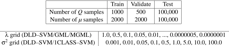
Train Validate Test

Number of Q samples 1000 500 100,000

Number of µ samples 2000 2000 100,000

λgrid (DLD–SVM/GML/MGML) 1.0, 0.5, 0.1, 0.05, 0.01, ..., 0.0000005, 0.0000001

σ2_{grid (DLD–SVM/1CLASS–SVM) 0.001, 0.01, 0.05, 0.1, 0.5, 1.0, 5.0, 10.0, 100.0}

Table 1: Parameters for experiments 1 and 2.

for all inverse covariance estimates and bothλand K are chosen to (approximately) minimize the

validation risk by searching a fixed grid of(λ,K)values.

Data for the first experiment are generated using an approach designed to mimic a type of real problem where x is a feature vector whose individual components are formed as linear combi-nations of raw measurements and therefore the central limit theorem is used to invoke a Gaussian

assumption for Q. Specifically, samples of the random variable x∼Q are generated by transforming

samples of a random variable u that is uniformly distributed over[0,1]27_{. The transform is x=Au}

where A is a 10–by–27 matrix whose rows contain between m=2 and m=5 non-zero entries with

value 1/m (i.e. each component of x is the average of m uniform random variables). Thus Q is

approximately Gaussian with mean(0.5,0.5) and support[0,1]10_{. Partial overlap in the nonzero}

entries across the rows of A guarantee that the components of x are partially correlated. We chose µ

to be the uniform distribution over[0,1]10_{. Data for the second experiment are identical to the first}

except that the vector(0,0,0,0,0,0,0,0,0,1)is added to the samples of x with probability 0.5. This

gives a bi-modal distribution Q that approximates a mixture of Gaussians. Also, since the support

of the last component is extended to[0,2]the corresponding component of µ is also extended to this

range. A summary of the data and algorithm parameters for experiments 1 and 2 is shown in Table 1. Note that the test set sizes are large enough to provide very accurate estimates of the risk.

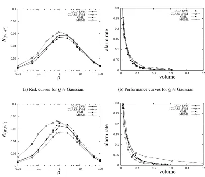
The four learning algorithms were applied for values ofρranging from.01 to 100 and the results

are shown in Figure 1. Figures 1(a) and 1(c) plot the empirical risk R_(W,W0₎versusρwhile Figures

1(b) and 1(d) plot the corresponding performance curves. Since the data is approximately Gaussian it is not surprising that the best results are obtained by GML (first experiment) and MGML (both

experiments). However, for most values ofρthe next best performance is obtained by DLD–SVM

(both experiments). The performance of 1CLASS–SVM is clearly worse than the other three at

smaller values ofρ(i.e. larger values of the volume), and this difference is more substantial in the

second experiment. In addition, although we do not show it, this difference is even more pronounced (in both experiments) at smaller training and validation set sizes. These results are significant

be-cause values ofρsubstantially larger than one appear to have little utility here since they yield alarm

rates that do not conform to our notion that anomalies are rare events. In additionρ1 appears

to have little utility in the general anomaly detection problem since it defines anomalies in regions where the concentration of Q is much larger than the concentration of µ, which is contrary to our premise that anomalies are not concentrated.

0 0.02 0.04 0.06 0.08 0.1

0.01 0.1 1 10 100

DLD–SVM 1CLASS–SVM GML MGML

ρ R(W

,

W

0)

(a) Risk curves for Q≈Gaussian.

0 0.05 0.1 0.15 0.2 0.25 0.3

0 0.1 0.2 0.3 0.4 0.5

DLD–SVM 1CLASS–SVM GML MGML volume ala rm ra te

(b) Performance curves for Q≈Gaussian.

0 0.02 0.04 0.06 0.08 0.1

0.01 0.1 1 10 100

DLD–SVM 1CLASS–SVM GML MGML

ρ R(W

,

W

0)

(c) Risk curves for Q≈Gaussian mixture.

0 0.05 0.1 0.15 0.2 0.25 0.3

0 0.1 0.2 0.3 0.4 0.5

DLD–SVM 1CLASS–SVM GML MGML volume ala rm ra te

(d) Performance curves for Q≈Gaussian mixture.

Figure 1: Synthetic data experiments.

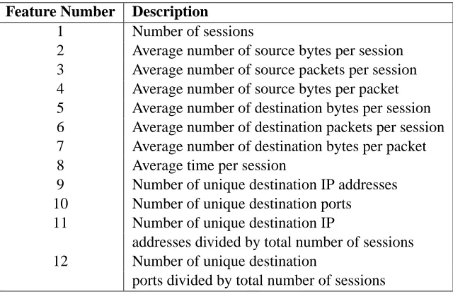
The averages were computed over one hour time windows giving a total of 11664 feature vectors.

The feature values were normalized to the range [0,1]and treated as samples from Q. Thus Q

has support in [0,1]12_{. Although we would like to choose µ to capture a notion of anomalous}

behavior for this application, only the DLD–SVM method allows such a choice. Thus, since both GML and MGML define densities with respect to a uniform measure and we wish to compare with

these methods, we chose µ to be the uniform distribution over[0,1]12_{. A summary of the data and}

algorithm parameters for this experiment is shown in Table 3. Again, we would like to point out that this choice may actually penalize the 1CLASS-SVM since this method is not based on the notion of a reference measure. However, we currently do not know any other approach which treats the 1CLASS-SVM with its special strucure in a fairer way.

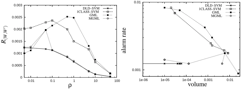
The four learning algorithms were applied for values ofρranging from.005 to 50 and the results

are summarized by the empirical risk curve in Figure 2(a) and the corresponding performance curve in Figure 2(b). The empirical risk values for DLD–SVM and MGML are nearly identical except for

Feature Number Description

1 Number of sessions

2 Average number of source bytes per session

3 Average number of source packets per session

4 Average number of source bytes per packet

5 Average number of destination bytes per session

6 Average number of destination packets per session

7 Average number of destination bytes per packet

8 Average time per session

9 Number of unique destination IP addresses

10 Number of unique destination ports

11 Number of unique destination IP

addresses divided by total number of sessions

12 Number of unique destination

ports divided by total number of sessions

Table 2: Outgoing network traffic features.

Train Validate Test

Number of Q samples 4000 2000 5664

Number of µ samples 10,000 100,000 100,000

λgrid (DLD–SVM/GML/MGML) 0.1, 0.01, 0.001, . . . , 0.0000001

σ2_{grid (DLD–SVM/1CLASS–SVM) 0.001, 0.01, 0.05, 0.1, 0.5, 1.0, 5.0, 10.0, 100.0}

(i.e. the MGML and GML solutions are identical atρ=0.05). Except for this case the empirical risk values for DLD–SVM and MGML are much better than 1CLASS–SVM and GML at nearly

all values of ρ. The performance curves confirm the superiority of DLD–SVM and MGML, but

also reveal differences not easily seen in the empirical risk curves. For example, all four methods

produced some solutions with identical performance estimates for different values of ρwhich is

reflected by the fact that the performance curves show fewer points than the corresponding empirical risk curves.

0 0.0005 0.001 0.0015 0.002 0.0025 0.003

0.01 0.1 1 10 100

DLD–SVM 1CLASS–SVM GML MGML

ρ R(W

,

W

0)

(a) Risk curves.

0.001 0.01

1e-06 1e-05 1e-04 0.001 0.01

DLD–SVM 1CLASS–SVM GML MGML

volume

ala

rm

ra

te

(b) Performance curves.

Figure 2: Cybersecurity experiment.

5. Discussion

A review of the literature on anomaly detection suggests that there are many ways to characterize anomalies (see e.g. Markou and Singh, 2003a,b). In this work we assumed that anomalies are not concentrated. This assumption can be specified by choosing a reference measure µ which determines

a density and a level valueρ. The density then quantifies the degree of concentration and the density

level ρestablishes a threshold on the degree that determines anomalies. Thus, µ andρ play key

roles in the definition of anomalies. In practice the user chooses µ andρto capture some notion of

anomaly that he deems relevant to the application.

This paper advances the existing state of “density based” anomaly detection in the following ways.

• Most existing algorithms make an implicit choice of µ (usually the Lebesgue measure) whereas

our approach allows µ to be any measure that defines a density. Therefore we accommodate a larger class of anomaly detection problems. This flexibility is in particular important when dealing with e.g. categorical data. In addition, it is the key ingredient when dealing with hidden classification problems, which we will discuss below.

• Prior to this work there have been no methods known to rigorously estimate the performance

namely the empirical classification risk, that enables such a comparision. In particular, it can be used to perform a model selection based on cross validation. Furthermore, the infinite sample version of this empirical performance measure is asymptotically equivalent to the standard performance measure for the DLD problem and under mild assumptions inequalities between them have been obtained.

• By interpreting the DLD problem as a binary classification problem we can use well-known

classification algorithms for DLD if we generate artificial samples from µ. We have demon-strated this approach which is a rigorous variant of a well-known heuristic for anomaly de-tection in the formulation of the DLD-SVM.

These advances have created a situation in which much of the knowledge on classification can now be used for anomaly detection. Consequently, we expect substantial advances in anomaly detection in the future.

Finally let us consider a different learning scenario in which anomaly detection methods are also commonly employed. In this scenario we are interested in solving a binary classification problem

given only unlabeled data. More precisely, suppose that there is a distribution νon X× {−1,1}

and the samples are obtained from the marginal distributionνX on X . Since labels exist but are

hidden from the user we call this a hidden classification problem (HCP). Hidden classification problems for example occur in network intrusion detection problems where it is impractical to obtain labels. Obviously, solving a HCP is intractable if no assumptions are made on the labeling process. One such assumption is that one class consists of anomalous, lowly concentrated samples (e.g. intrusions) while the other class reflects normal behaviour. Making this assumption rigorous

requires the specification of a reference measure µ and a threshold ρ. Interestingly, when νX is

absolutely continuous3with respect toν(.|y=1)solving the DLD problem with

Q := νX

µ := ν(.|y=1)

ρ := 2ν(X× {1})

gives the Bayes classifier for the binary classification problem associated with ν. Therefore, in

principle the DLD formalism can be used to solve the binary classification problem. In the HCP

however, although information about Q=νX is given to us by the samples, we must rely entirely

on first principle knowledge to guess µ andρ. Our inability to choose µ andρcorrectly determines

the model error that establishes the limit on how well the classification problem associated withν

can be solved with unlabeled samples. This means for example that when an anomaly detection

method is used to produce a classifier f for a HCP its anomaly detection performance

R

_P(f)with

P :=Q sµ and s := _1+ρ1 may be very different from its hidden classification performance

R

ν(f).

In particular

R

P(f)may be very good, i.e. very close to

R

P, while

R

ν(f)may be very poor, i.e. far

above

R

_ν. Another consequence of the above considerations is that the common practice of

mea-suring the performance of anomaly detection algorithms on (hidden) binary classification problems is problematic. Indeed, the obtained classification errors depend on the model error and thus they provide an inadequate description how well the algorithms solve the anomaly detection problem.

Furthermore, since the model error is strongly influenced by the particular HCP it is almost impos-sible to generalize from the reported results to more general statements on the hidden classification performance of the considered algorithms.

In conclusion although there are clear similiarities between the use of the DLD formalism for anomaly detection and its use for the HCP there is also an important difference. In the first case the

specification of µ andρdetermines the definition of anomalies and therefore there is no model error,

whereas in the second case the model error is determined by the choice of µ andρ.

Acknowledgments

We would like to thank J. Theiler who inspired this work when giving a talk on a recent paper (Theiler and Cai., 2003).

Appendix A. Regular Conditional Probabilities

In this apendix we recall some basic facts on conditional probabilities and regular conditional prob-abilities. We begin with

Definition 15 Let(X,

A

,P)be a probability space and

C

⊂

A

a sub-σ-algebra. Furthermore, let A∈

A

and g :(X,

C

)→Rbe P|C-integrable. Then g is called a conditional probability of A with

respect to

C

if

Z

C

1AdP =

Z

C

gdP

for all C∈

C

. In this case we write P(A|

C

):=g.

Furthermore we need the notion of regular conditional probabilities. To this end let (X,

A

)

and(Y,

B

)be measurable spaces and P be a probability measure on(X×Y,

A

⊗

B

). Denoting the

projection of X×Y onto X byπXwe writeπ−X1(

A

)for the sub-σ-Algebra of

A

⊗

B

which is induced

byπX. Recall, that this sub-σ-Algebra is generated by the collection of the sets A×Y , A∈

A

. For

later purpose, we also notice that this collection is obviously stable against finite intersections. Finally, PX denotes the marginal distribution of P on X , i.e. PX(A) =P(πX−1(A))for all A∈

A

.

Now let us recall the definition of regular conditional probabilities:

Definition 16 A map P(.|.):

B

×X →[0,1]is called a regular conditional probability of P if the following conditions are satisfied:

i) P(.|x)is a probability measure on(Y,

B

)for all x∈X .

ii) x7→P(B|x)is

A

-measurable for all B∈

B

.

iii) For all A∈

A

, B∈

B

we have

P(A×B) =

Z

A

P(B|x)PX(dx).

Theorem 17 If Y is a Polish space then a regular conditional probability P(.|.):

B

×X →[0,1]

of P exists.

Regular conditional probabilities play an important role in binary classification problems.

In-deed, given a probability measure P on X× {−1,1}the aim in classification is to approximately

find the set{P(y=1|x)>1

2}, where “approximately” is measured by the classification risk.

Let us now recall the connection between conditional probabilities and regular conditional prob-abilities (see Dudley, 2002, p. 342 and Thm. 10.2.1):

Theorem 18 If a conditional probability P(.|.):

B

×X→[0,1]of P exists then we P-a.s. have

P(B|x) = P X×B|π−_X1(

A

)

(x,y).

As an immediate consequence of this theorem we can formulate the following “test” for regular conditional probabilities.

Corollary 19 Let B∈

B

and f : X→[0,1]be

A

-measurable. Then f(x) =P(B|x)PX-a.s. if

Z

A×Y f◦πXdP= Z

A×Y1X×BdP

for all A∈

A

.

Proof The assertion follows from Theorem 18, the definition of conditional probabilities and the fact that the collection of the sets A×Y , A∈

A

is stable against finite intersections.

Appendix B. Proof of Proposition 9

Proof of Proposition 9 By Proposition 2 we have|2η−1|=

h−ρ h+ρ

and hence we observe

|2η−1| ≤t =

|h−ρ| ≤(h+ρ)t

=

−(h+ρ)t≤h−ρ≤(h+ρ)t

= n1−t

1+tρ≤h≤

1+t 1−tρ

o

,

whenever 0<t<1.

Now let us first assume that P has Tsybakov exponent q>0 with some constant C>0. Then

using

|h−ρ| ≤tρ =

(1−t)ρ≤h≤(1+t)ρ ⊂ n1−t

1+tρ≤h≤

1+t 1−tρ

o

we find

PX

|h−ρ| ≤tρ ≤ PX

|2η−1| ≤t ≤ Ctq,

Now let us conversely assume that h has ρ-exponent q with some constant C>0. Then for 0<t<1 we have

Q |h−ρ| ≤t =

Z

X

1{|h−ρ|≤t}hdµ

=

Z

{h≤1+ρ}1{|h−ρ|≤t}hdµ

≤ (1+ρ)

Z

{h≤1+ρ}

1_{{|h−ρ|≤t}}dµ

= (1+ρ)µ |h−ρ| ≤t .

Using PX=_ρ+11 Q+_ρ+1ρ µ we hence find

PX

|h−ρ| ≤t ≤ 2µ |h−ρ| ≤t ≤ 2Ctq

for all sufficiently small t∈(0,1). Let us now define tl:=₁₊2t_t and tr:=₁2t_−t. This immediately gives

1−tl=1₁₊−t_t and 1+tr=1+_1−tt. Furthermore, we obviously also have tl ≤tr. Therefore we find

n1−t

1+tρ≤h≤

1+t 1−tρ

o

=

(1−tl)ρ≤h≤(1+tr)ρ

⊂

(1−tr)ρ≤h≤(1+tr)ρ

=

|h−ρ| ≤trρ .

Hence for all sufficiently small t>0 with t< 1

1+2ρ, i.e. trρ<1, we obtain

PX

|2η−1| ≤t ≤ PX

|h−ρ| ≤trρ ≤ 2C(trρ)q ≤ 2C(1+2ρ)qtq.

From this we easily get the assertion.

References

S. Ben-David and M. Lindenbaum. Learning distributions by their density levels: a paradigm for learning without a teacher. J. Comput. System Sci., 55:171–182, 1997.

C. Campbell and K. P. Bennett. A linear programming approach to novelty detection. In T. K. Leen, T. G. Dietterich, and V. Tresp, editors, Advances in Neural Information Processing Systems 13, pages 395–401. MIT Press, 2001.

C.-C. Chang and C.-J. Lin. LIBSVM: a library for support vector machines, 2004.

A. Cuevas, M. Febrero, and R. Fraiman. Cluster analysis: a further approach based on density estimation. Computat. Statist. Data Anal., 36:441–459, 2001.

M. J. Desforges, P. J. Jacob, and J. E. Cooper. Applications of probability density estimation to the detection of abnormal conditions in engineering. Proceedings of the Institution of Mechanical Engineers, Part C—Mechanical engineering science, 212:687–703, 1998.

R. O. Duda, P. E. Hart, and D. G. Stork. Pattern Classification. Wiley, New York, 2000.

R. M. Dudley. Real Analysis and Probability. Cambridge University Press, 2002.

W. Fan, M. Miller, S. J. Stolfo, W. Lee, and P. K. Chan. Using artificial anomalies to detect unknown and known network intrusions. In IEEE International Conference on Data Mining (ICDM’01), pages 123–130. IEEE Computer Society, 2001.

F. Gonz´alez and D. Dagupta. Anomaly detection using real-valued negative selection. Genetic Programming and Evolvable Machines, 4:383–403, 2003.

J. A. Hartigan. Clustering Algorithms. Wiley, New York, 1975.

J. A. Hartigan. Estimation of a convex density contour in 2 dimensions. J. Amer. Statist. Assoc., 82: 267–270, 1987.

P. Hayton, B. Sch¨olkopf, L. Tarassenko, and P. Anuzis. Support vector novelty detection applied to jet engine vibration spectra. In T. K. Leen, T. G. Dietterich, and V. Tresp, editors, Advances in Neural Information Processing Systems 13, pages 946–952. MIT Press, 2001.

S. P. King, D. M. King, P. Anuzis, K. Astley, L. Tarassenko, P. Hayton, and S. Utete. The use of nov-elty detection techniques for monitoring high-integrity plant. In IEEE International Conference on Control Applications, pages 221–226. IEEE Computer Society, 2002.

E. Mammen and A. Tsybakov. Smooth discrimination analysis. Ann. Statist., 27:1808–1829, 1999.

C. Manikopoulos and S. Papavassiliou. Network intrusion and fault detection: a statistical anomaly approach. IEEE Communications Magazine, 40:76–82, 2002.

M. Markou and S. Singh. Novelty detection: a review—Part 1: statistical approaches. Signal Processing, 83:2481–2497, 2003a.

M. Markou and S. Singh. Novelty detection: a review—Part 2: neural network based approaches. Signal Processing, 83:2499–2521, 2003b.

D. W. M¨uller and G. Sawitzki. Excess mass estimates and tests for multimodality. J. Amer. Statist. Assoc., 86:738–746, 1991.

A. Nairac, N. Townsend, R. Carr, S. King, P. Cowley, and L. Tarassenko. A system for the analysis of jet engine vibration data. Integrated Computer-Aided Engineering, 6:53–56, 1999.

W. Polonik. Measuring mass concentrations and estimating density contour clusters—an excess mass aproach. Ann. Statist., 23:855–881, 1995.

G. Sawitzki. The excess mass approach and the analysis of multi-modality. In W. Gaul and D. Pfeifer, editors, From data to knowledge: Theoretical and practical aspects of classification, data analysis and knowledge organization, Proc. 18th Annual Conference of the GfKl, pages 203–211. Springer, 1996.

B. Sch¨olkopf, J. C. Platt, J. Shawe-Taylor, and A. J. Smola. Estimating the support of a high-dimensional distribution. Neural Computation, 13:1443–1471, 2001.

B. Sch¨olkopf and A. J. Smola. Learning with Kernels. MIT Press, 2002.

I. Steinwart. On the influence of the kernel on the consistency of support vector machines. J. Mach. Learn. Res., 2:67–93, 2001.

I. Steinwart. Consistency of support vector machines and other regularized kernel machines. IEEE Trans. Inform. Theory, 51:128–142, 2005.

I. Steinwart and C. Scovel. Fast rates for support vector machines using Gaussian kernels. Ann. Statist., submitted, 2004. http://www.c3.lanl.gov/˜ingo/publications/ann-04a.pdf.

L. Tarassenko, P. Hayton, N. Cerneaz, and M. Brady. Novelty detection for the identification of masses in mammograms. In 4th International Conference on Artificial Neural Networks, pages 442–447, 1995.

J. Theiler and D. M. Cai. Resampling approach for anomaly detection in multispectral images. In Proceedings of the SPIE 5093, pages 230–240, 2003.

A. B. Tsybakov. On nonparametric estimation of density level sets. Ann. Statist., 25:948–969, 1997.

A. B. Tsybakov. Optimal aggregation of classifiers in statistical learning. Ann. Statist., 32:135–166, 2004.

D. Y. Yeung and C. Chow. Parzen-window network intrusion detectors. In Proceedings of the 16th International Conference on Pattern Recognition (ICPR’02) Vol. 4, pages 385–388. IEEE Computer Society, 2002.