Importance Sampling for Continuous Time Bayesian Networks

Importance Sampling for Continuous Time Bayesian Networks

Yu Fan [email protected]

Jing Xu [email protected]

Christian R. Shelton [email protected]

Department of Computer Science and Engineering University of California

Riverside, CA, 92521, USA

Editor: Carl Edward Rasmussen

Abstract

A continuous time Bayesian network (CTBN) uses a structured representation to describe a dynamic sys-tem with a finite number of states which evolves in continuous time. Exact inference in a CTBN is often intractable as the state space of the dynamic system grows exponentially with the number of variables. In this paper, we first present an approximate inference algorithm based on importance sampling. We then extend it to continuous-time particle filtering and smoothing algorithms. These three algorithms can estimate the ex-pectation of any function of a trajectory, conditioned on any evidence set constraining the values of subsets of the variables over subsets of the time line. We present experimental results on both synthetic networks and a network learned from a real data set on people’s life history events. We show the accuracy as well as the time efficiency of our algorithms, and compare them to other approximate algorithms: expectation propagation and Gibbs sampling.

Keywords: continuous time Bayesian networks, importance sampling, approximate inference, filtering, smoothing

1. Introduction

Many real world applications involve highly complex dynamic systems. These systems usually contain a large number of stochastic variables, which evolve asynchronously in continuous time. Such dynamic sys-tems include computer networks, sensor networks, social networks, mobile robots, and cellular metabolisms. Modeling, learning and reasoning about these complex dynamic systems is an important task and a great challenge.

1.1 Structured Process Representation

A central task of the above applications is to calculate probability distributions of the system over time. For instance, we may wish to know the distribution over when a variable will change next or the state of a current variable, given past (partial) evidence. However, as the number of the variables increases, the state space of the distribution grows exponentially. Such growth makes the inference task very difficult for large systems. One solution is to use structured representation to factorize the state space according to the dependencies of the variables. For dynamic systems, Dynamic Bayesian Networks (DBNs) (Dean and Kanazawa, 1989) are commonly used. A DBN describes the dynamic system as a time-sliced model by measuring the evolution of the system with a (usually fixed) time interval∆t . The transition probabilities from states at time t to states

at time t+∆t are represented by a Bayesian network. DBNs can work well for systems that are observed at

regular time steps. However, for many applications, discretizing time has several limitations. First, we usually choose a fixed time interval,∆t. In many real world systems, variables evolve at different time granularities.

Some variables may evolve very fast whereas some evolve very slowly. Choosing an appropriate time interval is a difficult task. Larger∆t may result in an inaccurate model while smaller∆t may cause inference in the

Second, the dependencies of the transition model are unstable with respect to∆t. That is, different choices

of ∆t may result in different network structures between t and t+∆t. The network structure represents

independencies between variables at t and∆t. This is a function of∆t, both theoretically and empirically

(Nodelman et al., 2003). If∆t is an inherent parameter of the process, this is not a problem. However, if it

is chosen for estimation or computational reasons, this becomes an issue as its choice is not unique. Finally, DBNs (and discrete-time Markov processes in general) do not necessarily correspond to processes that are Markovian outside of the sampled instants of time. Consider that if T is the transition matrix for a process with time interval∆t, T1/2is the transition matrix for the same process with time interval∆₂t. However, such a square root may not exist in the space of real matrices. Therefore, there may not be any simple extension of a DBN to the times between the sampled instants.

An alternative and more natural approach to model dynamic systems is to use a continuous-time model. For systems with a finite number of states, one way is to consider the entire system as a continuous-time discrete-state Markov process. Like discrete-time processes, this method suffers from the fact that the state space of the process grows exponentially with the number of variables in the system. Recently, Nodelman et al. (2002) extended this framework to a continuous time Bayesian network (CTBN), which factorizes a system into local variables using a graphical representation, much as a DBN does for a discrete-time pro-cess. Parameter estimation in CTBNs with fully observed data and partially observed data were provided in Nodelman et al. (2003) and Nodelman et al. (2005b) respectively. Because CTBNs explicitly represent the temporal dynamics in continuous time and explore the dependencies among stochastic variables using a structured representation, they have been applied to various real world systems, including human-computer interactions (Nodelman and Horvitz, 2003), server farm failures (Herbrich et al., 2007), robot monitoring (Ng et al., 2005) and network intrusion detection (Xu and Shelton, 2008). Kan and Shelton (2008) used the CTBN representation in their solution of structured continuous-time Markov decision processes.

Queueing theory (Bolch et al., 1998) and Petri nets (Petri, 1962) provide an alternative continuous-time structured process models. However, they make different assumptions about the structure. They were de-signed to answer questions about steady-state distributions. Their algorithms are not suited to learning from partial data nor to answering many statistical questions. A singular and recent exception is the work of Sutton and Jordan (2008) which applied Gibbs sampling to queueing models.

1.2 Prior CTBN Inference Methods

In CTBNs, a trajectory (or sample) consists of the starting values for the system along with the (real-valued) times at which the variables change and their corresponding new values. Inference for a CTBN is the task of estimating the distribution over trajectories given a partial trajectory (in which some values or transitions are missing for some variables during some time intervals). Inference plays a central role as it not only helps us answer queries about distributions, but it is also involved in parameter estimation when the observation data is incomplete. Performing exact inference in a CTBN requires constructing a single rate matrix for the entire system and computing the exponential of the matrix, which is often intractable: the exponentiation must be performed separately for each period of constant evidence and (more problematic) even a sparse rep-resentation of the matrix may not fit in memory. Thus, many applications of CTBNs require an approximate inference method. A method based on expectation propagation (Minka, 2001) was presented in Nodelman et al. (2005a). Saria et al. (2007) extended it to full belief propagation and provided a method to adapt the approximation quality.

Other approximate inference methods are based on sampling. They have the advantage of being anytime algorithms. (We can stop at any time during the computation and obtain an answer.) Furthermore, in the limit of infinite samples (computation time), they converge to the true answer.

As we note below, because time is a continuous variable, any evidence containing a record of the change in a variable has a zero probability under the model. Therefore rejection sampling and straightforward likelihood weighting are generally not viable methods.

incor-poration of evidence from a continuous-state part of the system (which we do not consider here). Recently, El-Hay et al. (2008) provided another sampling algorithm for CTBNs using Gibbs sampling. The algorithm starts from an arbitrary trajectory that is consistent with the evidence. Then, in each iteration, it randomly picks one variable X , and samples an entire trajectory for that variable by fixing the trajectory of all the other variables. Since only X is not fixed, the conditioned cumulative distribution that X stays in one state less than t and the state transition probabilities can be calculated exactly using standard forward and backward propagation within the Markov blanket of X . The Gibbs sampling algorithm can handle any type of evidence and it provides an approach to sample from the exact posterior distribution given the evidence. However, the posterior distribution can be any arbitrary function. To sample exactly from it, binary search has to be applied and F(t)is repeatedly evaluated, which may affect the efficiency of the algorithm.

1.3 Outline of This Work

In this paper we explore a different sampling approach using importance sampling. Our algorithm generates weighted samples to approximate the expectation of a function of the trajectory. It differs from previous approaches in a number of key ways. There is no exact inference method involved in our approach. Thus, our algorithm does not depend on complex numeric computations. The transition times for variables are sampled from regular exponential distributions in our algorithm, which can be done in constant time. Our algorithm can be adapted to a population-based filter (a particle filter). It can handle both point and continuous evidence, is simple to implement, and can be easily extended to continuous time systems other than CTBNs. The formulation of this sampling procedure is not trivial due to the infinite extent of the trajectory space, both in the transition time continuum and the number of transitions. The algorithm was first presented in Fan and Shelton (2008). This paper extends that work by comparing the algorithm to the newly developed Gibbs sampling algorithm (El-Hay et al., 2008), evaluating its performance on parameter learning with partially observed data, and demonstrating its performance on real-world networks.

The remainder of the paper is structured as follows. In Section 2, we briefly describe the notation for CTBNs. In Section 3, we describe our importance sampling algorithm for CTBNs and extend the algorithm to particle filtering and particle smoothing algorithms. In Section 4, we describe our experiment results.

2. Continuous Time Bayesian Networks

We first briefly describe the definition, likelihood, and sufficient statistics of the CTBN model. We then review the exact inference and parameter estimation algorithms for CTBNs.

2.1 The CTBN Model

Continuous time Bayesian networks (Nodelman et al., 2002) are based on the framework of continuous time, finite state, homogeneous Markov processes (Norris, 1997). Let X be a continuous time, finite state, homo-geneous Markov process with n states_{x1, . . . ,xn}. The behavior of X is described by the initial distribution

P_X0and the transition model which is often represented by the intensity matrix

QX=

    

−qx1 qx1x2 ··· qx1xn qx2x1 −qx2 ··· qx2xn

..

. ... . .. ...

qxnx1 qxnx2 ··· −qxn     ,

Exercise

Weather Body Weight

Calorie Intake

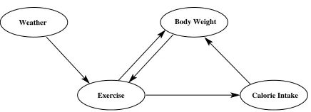
Figure 1: CTBN Example: Weight Control Effect

are

f(qxi,t) =qxiexp(−qxit), t≥0.

F(qxi,t) =1−exp(−qxit), t≥0.

The expected time of transitioning is 1/qxi. Upon transitioning, the probability X transitions from state xito xjisθxixj =qxixj/qxi.The distribution over the state of X at time t can be calculated as

PX(t) =PX0exp(QXt)

where P0

Xis the distribution over X at time 0 represented as a row vector, and exp is the matrix exponential. To model a dynamic system containing several variables, we can consider the whole system as one vari-able, enumerate the entire state space, calculate the transition intensity of each pair of these states and put them into a single intensity matrix. However, the size of the state space grows exponentially with the number of variables in the system, which makes this method infeasible for large systems.

Nodelman et al. (2002) defined a continuous time Bayesian network (CTBN), which uses a graphical model to provide a compact factored representation of continuous time Markov process. A CTBN models each local variable X as an inhomogeneous Markov process, whose parametrization depends on some subset of other variables U. The intensity matrix of X is called a conditional intensity matrix (CIM) QX_|U, which is defined as a set of intensity matrices QX_|u, one for each instantiation u of the variable set U. The evolution of X depends instantaneously on the values of the variables in U.

LetXbe a dynamic system containing several variables X . A continuous time Bayesian network

N

X, specified as a Bayesian network

B

G

G

Q_X|UX.

Example 1 Assume we want to model the behavior of a person controlling his body weight. When the person is overweight, he may exercise more to lose the excess weight. Increasing exercise intensity tends to increase his appetite, which will increase his daily calorie intake. Both exercise intensity and calorie intake contribute to his body weight. Furthermore, the exercise intensity also depends on the weather. Such a dynamic system contains four variables: body weight, exercise, calorie intake, and weather. Each variable changes in continuous time and its change rate depends on the current value of some other variables.

We can use a CTBN to represent such behavior. The dependencies of these four variables are depicted using a graphical structure, as shown in Figure 1. The quantitative transient dynamics for each variable is represented using a conditional intensity matrix. Let us assume all the four variables are binary. Let B(t) be the person’s body weight ( Val(B(t)) ={b0=normal,b1=overweight}), E(t)be the exercise intensity

(Val(E(t) ={e0=light,e1=heavy}), C(t)be his daily calorie intake ( Val(C(t) ={c0=low,c1=high})

and W(t)be the weather ( Val(W(t) ={w0=rainy,w1=sunny}). The conditional intensity matrices for the

QW QW =

−0.5 0.5 0.5 ₋0.5

,

QE_|W,B

Q_E|w0,b0 =

−0.1 0.1

2 ₋2

, Q_E|w1,b0 =

−0.3 0.3

1 ₋1

,

Q_E|w0,b1 =

−0.5 0.5 0.5 ₋0.5

, Q_E|w1,b0 =

−1 1

0.1 ₋0.1

,

Q_C|E Q_C|e0 =

−0.2 0.2

1 ₋1

, Q_C|e1 =

−1 1

0.2 ₋0.2

,

Q_B|E,C

QB|e0,c0 =

−0.2 0.2 0.8 ₋0.8

, QB|e1,c0 =

−0.1 0.1

1 ₋1

,

Q_B|e 0,c1 =

−1 1

0.1 ₋0.1

, Q_B|e 1,c1 =

−0.2 0.2 0.6 ₋0.6

.

Notice that unlike Bayesian networks, the CTBN model allows cycles. The transient behavior of each local variable is controlled by the current value of its parents. If the person is doing light exercise and his calorie intake is low, the dynamics of his body weight are determined by the intensity matrix Q_B|e0,c0. If the time unit is one month, we expect his weight will go back to normal in 1/0.8=1.25 months if he is currently

overweight and doing light exercise and controlling his daily calorie intake.

We can also use a single continuous time Markov process to represent this network, which requires an intensity matrix of size 16_×16. To generate the single intensity matrix, we can follow the amalgamation

algorithm in Nodelman et al. (2002). Basically, we enumerate the entire state space(W,E,C,B), and assign intensity 0 to transitions that change two variables simultaneously. For any transition involving only one of the variables, simply use the entry from the appropriate intensity matrix above. The resulting matrix is

w0e0c0b0

                         

−1 0.5 0.1 0 0.2 0 0 0 0.2 0 0 0 0 0 0 0

0.5 ₋1.2 0 0.3 0 0.2 0 0 0 0.2 0 0 0 0 0 0

2 0 −3.6 0.5 0 0 1 0 0 0 0.1 0 0 0 0 0

0 1 0.5 −2.6 0 0 0 1 0 0 0 0.1 0 0 0 0

1 0 0 0 −2.6 0.5 0.1 0 0 0 0 0 1 0 0 0

0 1 0 0 0.5 −2.8 0 0.3 0 0 0 0 0 1 0 0

0 0 0.2 0 2 0 ₋2.9 0.5 0 0 0 0 0 0 0.2 0

0 0 0 0.2 0 1 0.5 −1.9 0 0 0 0 0 0 0 0.2

0.8 0 0 0 0 0 0 0 −2 0.5 0.5 0 0.2 0 0 0

0 0.8 0 0 0 0 0 0 0.5 −2.5 0 1 0 0.2 0 0

0 0 1 0 0 0 0 0 0.5 0 −3 0.5 0 0 1 0

0 0 0 1 0 0 0 0 0 0.1 0.5 ₋2.6 0 0 0 1

0 0 0 0 0.1 0 0 0 1 0 0 0 −2.1 0.5 0.5 0

0 0 0 0 0 0.1 0 0 0 1 0 0 0.5−2.6 0 1

0 0 0 0 0 0 0.6 0 0 0 0.2 0 0.5 0 −1.8 0.5

0 0 0 0 0 0 0 0.6 0 0 0 0.2 0 0.1 0.5 −1.4

                           .

w1e0c0b0

w0e1c0b0

w1e1c0b0

w0e0c1b0

w1e0c1b0

w0e1c1b0

w1e1c1b0

w0e0c0b1

w1e0c0b1

w0e1c0b1

w1e1c0b1

w0e0c1b1

w1e0c1b1

w0e1c1b1

w1e1c1b1

As we include more variables in this system, the size of the intensity matrix grows exponentially with the number of variables.

2.2 Likelihood and Sufficient Statistics

ofσ(Nodelman et al., 2003). Let T[x_|u]be the amount of time X=x while UX=u, and M[x,x′|u]be the number of transitions from x to x′while UX=u. If we let M[x|u] =∑x′M[x,x′|u], the probability density of trajectoryσ(omitting the starting distribution) is

P_N(σ) =

∏

X∈X

LX(T[X|UX],M[X|UX]) (1)

where

LX(T[X|UX],M[X|UX]) =

∏

∏

qM_x|u[x|u]exp(−q_x|uT[x_|u])

∏

x′6=x

θM[x,x′|u]

xx′_|u

!

(2)

is the local likelihood for variable X . The likelihood also decomposes by time. That is, the likelihood of a trajectory on[0,T)is equal to the likelihood based only on sufficient statistics from time 0 to time t multiplied by the likelihood based only on sufficient statistics from time t to time T .

2.3 Evidence and Queries

Given a CTBN model, we would like to use it to answer queries conditioned on observations. There are two common types of observations: point evidence and continuous evidence. Point evidence represents the observation of the value of some variables at a particular time instant. Continuous evidence provides the behavior of some variables throughout an interval[t1,t2). For instance, x=1 during the interval[2,3.5), or

x=1 from t=2 to t=3 and then x transitions to x=0 at t=3 and stays in that state until t=5. We define

x[t1: t2)be the behavior of variable X on the interval[t1,t2), x[t1: t2]be the behavior of X on the interval

[t1,t2]and x(t1: t2]be the behavior of X on the interval(t1,t2].

Queries can ask about the marginal distribution of some variables at a particular time, such as the dis-tribution of x and y at t=2, or questions about the timing of a transition, such as the distribution over the time that y transitions from y=1 to y=2 for the first time in the interval[1,4). In learning (especially when employing expectation-maximization), we might query the expected sufficient statistics of a CTBN, which include the total amount of time that a variable spends in a state, and the total number of times that a variable transitions from one state to another state under certain conditions. For example, we might want to know the total amount of time that x=0 throughout the entire interval, or the number of times that x transitions from 1 to 2 during the time interval[2,3)when y=0. In this paper, we will concentrate on answering queries given the continuous evidence, but our method can be trivially extended to point evidence.

2.4 Exact Inference in CTBNs

A CTBN can be viewed as a homogeneous Markov process with a large joint intensity matrix amalgamated from the CIMs of the CTBN. Exact inference in a CTBN can be performed by generating a single joint intensity matrix over the entire state space of the CTBN and running the forward-backward algorithm on the joint intensity matrix of the homogeneous Markov process. We review this method here, but a more complete treatment can be found in Nodelman et al. (2002).

Assume that we have a partially observed trajectoryσof a CTBN

N

To perform exact inference, we first generate the intensity matrix Q for the joint homogeneous Markov process and incorporate the evidence into Q. If each variable Xiin the CTBN

N

qi jin Q for which only one variable value is different between states i and j is the corresponding intensity in the CIM of that variable. All the other off-diagonal elements are zero since two variables can not transition at exactly the same time in a CTBN. The diagonal elements are computed to make each row sum to zero.

Addi-tionally, let Qi,jbe the matrix Q with all elements zeroed out except the off-diagonal elements that represent the intensities of transitioning from non-zero rows in Qi to non-zero columns in Qj. If evidence blocks i and j differs only in which variables are observed (no transition is observed between them), then Qi,j is the identity matrix instead.

exp(Qi(ti+1−ti))represents the transition matrix for interval[ti,ti+1)and Qi,i+1corresponds to the tran-sition probability density between two consecutive intervals at time ti+1. We can use the forward-backward algorithm for Markov process to answer queries.

We define the forward and backward probability vectorsαtandβtas

αt = p(Xt,σ[0,t)),

βt = p(σ[t,T)|Xt).

Letα0be the initial distribution PX0over the state andβT be a vector of ones. The forward and backward distribution vector for each interval can be calculated recursively:

α_ti+1 = α_tiexp(Qi(ti+1−ti))Qi,i+1,

βti = Qi−1,iexp(Qi(ti+1−ti))βti+1.

The distribution over the state of the CTBN at time t_∈[ti,ti+1)given the evidenceσ[0,T)can be computed as

P(Xt=k,σ[0,T)) =αtiexp(Qi(t−ti))∆k,kexp(Qi(ti+1−t))βti+1 (3)

where _∆i,j is an n×n matrix of zeros with a single one in position i,j. Other queries can be similarly computed.

2.5 CTBN Parameter Estimation

Given a set of trajectories D={σ1,σ2, . . . ,σn}and a fixed graphical structure, we would like to estimate the parameters (the conditional intensity matrix) of the CTBN model.

When the data set D is complete, where each trajectoryσi is a complete set of state transitions and the times at which they occurred, the parameters can be learned by maximizing the log-likelihood of the data set (Nodelman et al., 2003). According to Equation 1 and Equation 2, the log-likelihood can be written as the sum of the log-likelihood for each local variable. By maximizing the log-likelihoods, the parameters can be derived as

ˆ

qx_|u=

M[x_|u]

T[x_|u]; θˆxx′|u=

M[x,x′_|u]

M[x_|u] . (4)

When the data set is incomplete, the expectation maximization (EM) algorithm (Dempster et al., 1977) can be used to find the maximum likelihood parameters (Nodelman et al., 2005b). The EM algorithm begins with an arbitrary initial parameter assignment, and alternatively repeats the expectation step and maximization step until convergence. In expectation step, for each trajectoryσi∈D, expected sufficient statistics ¯M[x|u],

¯

M[x,x′_|u]and ¯T[x_|u]are computed using exact inference. In maximization step, new parameters are computed according to Equation 4 as if the expected sufficient statistics came from complete data.

3. Sampling-based Inference

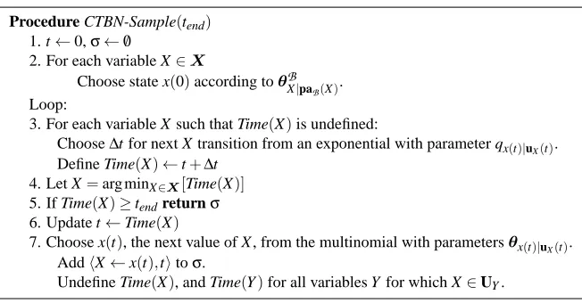
Procedure CTBN-Sample(tend) 1. t←0,σ←/0

2. For each variable X∈X

Choose state x(0)according toθB

X_|pa_B(X).

Loop:

3. For each variable X such that Time(X)is undefined:

Choose∆t for next X transition from an exponential with parameter qx(t)|uX(t).

Define Time(X)←t+∆t

4. Let X=arg minX_∈X[Time(X)]

5. If Time(X)≥tendreturnσ 6. Update t←Time(X)

7. Choose x(t), the next value of X , from the multinomial with parametersθ_x(t) |uX(t).

Add_hX_←x(t),t_itoσ.

Undefine Time(X), and Time(Y)for all variables Y for which X∈UY.

Figure 2: Forward sampling semantics for a CTBN

3.1 Forward Sampling

Queries that are not conditioned on evidence can be answered by randomly sampling many trajectories and looking at the fraction that match the query. More formally, if we have a CTBN

N

D

D

ˆ

E_N[g] = 1 M

M

∑

m=1

g(σ[m]). (5)

For example, if we let g=1{x(5) =x1}then we could use the above formula to estimate PN(x(5) =x1). Or the function g(σ)might count the total number of times that X transitions from x1to x2while its parent U has value u1, allowing us to estimate the expected sufficient statistic M[x1,x2|u1]. The algorithm for sampling a trajectory is shown in Figure 2. For each variable X_∈X, it maintains x(t)—the state of X at time t—and

Time(X)—the next potential transition time for X . The algorithm adds transitions one at a time, advancing

t to the next earliest variable transition. When a variable X (or one of its parents) undergoes a transition, Time(X)is resampled from the new exponential waiting time distribution. We use uX(t)to represent the instantiation to parents of X at time t.

If we want to obtain a conditional probability of a query given evidence, the situation is more complicated. We might try to use rejection sampling: forward sample to generate possible trajectories, and then simply reject the ones that are inconsistent with our evidence. The remaining trajectories are sampled from the posterior distribution given the evidence, and can be used to estimate probabilities as in Equation 5. However, this approach is entirely impractical in our setting, as in any setting involving an observation of a continuous quantity—in our case, time. In particular, suppose we observe that X transitions from x1to x2at time t. The probability of sampling a trajectory in which that transition occurs at precisely that time is zero. Thus, if we have evidence about transitions, with probability 1, none of our sampled trajectories will be relevant.

3.2 Gibbs Sampling

Recently, El-Hay et al. (2008) provided a Markov Chain Monte Carlo (MCMC) procedure which used a Gibbs sampler to generate samples from the posterior distribution given the evidence.

Suppose we want to sample trajectories from a CTBN with n variables(Xi,X2, . . . ,Xn)given the evidence

e. The Gibbs sampler starts with an arbitrary trajectory that is consistent with the evidence. In each iteration,

of the other variables Y ={X1, . . . ,Xi−1,Xi+1, . . . ,Xn} as evidence. To generate the entire trajectory of Xi according to the evidence e, the states and transitions of Xineed to be sampled in those intervals that Xiis not observed according to the evidence. The trajectory in each unobserved interval of Xi can be generated by alternatively sampling transition time∆t and new state x from the posterior distribution given e and the

trajectories of the other variables Y .

Assume we are sampling the trajectory of X for the interval [0,T], and Xi(0) =x0, Xi(T) =xT. The transition time∆t is sampled by inverse transform sampling: first drawξfrom the[0,1]uniform distribution and set∆t=F−1(ξ), where F−1(ξ)is the inverse of the conditional cumulative distribution function F(t)

that Xistays in state x0for a time less than t:

F(t) =1₋Pr(Xi(0 : t] =x0|x0,xT,Y[0 : T]).

F(t)can be calculated by decomposing Pr(Xi(0 : t] =x0|x0,xT,Y[0 : T])using the Markov property of the process:

Pr(Xi(0 : t] =x0|x0,xT,Y[0 : T]) = ˜

α(t)β˜x0(t) ˜ βx0(0) where

˜

α(t) =Pr(Xi(0 : t] =x0,Y[0 : t]|x0,Y0), ˜

βx(t) =Pr(xT,Y(t : T]|Xi(t) =x,Y(t)).

˜

α(t)and ˜βx(t)can be calculated using a slightly modified version of the standard forward-backward algorithm described in Section 2.4. Using the fact that Xi is independent of all the other components given the entire trajectory of its Markov blanket, the computation of ˜α(t)and ˜β(t)can be limited to Xiand its Markov blanket (the parents of Xi, the children of Xi, and the children’s parents).

Since the conditional cumulative distribution function F(t)can be arbitrarily complex, the inverse func-tion F−1(t)can not be solved analytically. Finding∆t that satisfies F(∆t) =ξis performed using a two-step searching method: first find the interval[τk,τk+1]that satisfies F(τk)<ξ<F(τk+1), whereτkare the tran-sition points of the Markov blanket of Xi. Then ∆t is found by performing an L step binary search on the interval[τk,τk+1].

The transition probability that Xitransitions from x(0)to a new state x can be calculated similarly:

Pr(Xi(t+) =x|Xi(0 : t] =x(0),Y(0 : T]) =

qXi|Y

x0,xβ˜x(t)

∑x′₆=x0q

Xi|Y

x0,x′

˜ βx′(t)

.

The Gibbs sampling algorithm can handle any type of evidence. The sampled trajectories are guaranteed to be consistent with the evidence. However, sampling the transition time∆t requires using a binary search

algorithm and repeatedly computing the conditional cumulative distribution function F(t), which may require long running time.

3.3 Importance Sampling

In this section, we introduce another approximate inference method using importance sampling, which does not require computing the exact posterior distribution. This method first appeared in Fan and Shelton (2008). In importance sampling, we generate samples from a proposal distribution P′which guarantees that our sampled trajectories will conform to our evidence e. We must weight our samples to correct for the fact that we are drawing them from P′instead of the target distribution P_N defined by the CTBN. In particular, ifσis a sample from P′we set its weight to be

w(σ) =PN(σ,e)

In normalized importance sampling, we draw a set of samples

D

ˆ

E_N[g_|e] = 1 W

M

∑

m=1

g(σ[m])w(σ[m])

where W is the sum of the weights.

This estimator is consistent if the support of P′ is a superset of the support of P_N. In general, ˆE_N is biased and the bias decreases as O(M−1). The variance of the estimator also decreases as O(M−1). For more information on this and related sampling estimates, see Hesterberg (1995).

For our algorithm, we base the proposal distribution on the forward sampling algorithm. As we are sampling a trajectory, we occasionally depart from the regular forward sampling algorithm and “force” the behavior of one or more variables to ensure consistency with the evidence.

3.4 Simple Evidence

The simplest query involves evidence over some subset of variablesV _⊂X for the total length of the tra-jectory. We force only the behavior of the variablesV and there are no choices about how to do that. In particular, we use the following proposal distribution: forward sample the behavior of variables X_∈(X_\V)

inserting the known transitions at known times for variables inV as determined by the evidence. As there are no choices in our forcing, the likelihood of drawingσfrom the proposal distribution is just the likeli-hood contribution of forward sampling the behavior of the variables X_∈(X_\V), in the context of the total behavior of the system.

According to Section 2.2, x[t1: t2)can be summarized by the sufficient statistics over X on the inter-val[t1,t2). Let ˜LX(x[t1: t2))be a partial likelihood contribution function, computed by plugging the suf-ficient statistics of x[t1: t2) into Equation 2. The partial contribution function can be defined over a col-lection of intervals

I

I

1: t2)∈I˜LX(x[t1: t2)). Returning to our simple evidence above, let τ1<τ2. . . ,τn−1<τnbe all the transition times inσ[0,T),τ0=0 andτn+1=T . The likelihood of drawingσ from the target distribution P_N is

˜L_N(σ) =

∏

X_∈X

n

∏

i=0

˜LX(x[τi:τi+1))

Let ˜L′_X(x[t1: t2))be the corresponding probability density for our sampling procedure. Since we force the values and transitions of variables inV according to the evidence, the probability that we sample an interval

x[τi:τi+1)for X∈V from proposal distribution P′is always 1. Therefore, the likelihood of drawingσfrom the proposal distribution P′is

˜L′

N(σ) =

∏

X∈X

n

∏

i=0

˜L′

X(x[τi:τi+1))

=

∏

X∈(X_\V₎

n

∏

i=0

˜LX(x[τi:τi+1))×

∏

X_∈V

n

∏

i=0

1.

To compute the proper weight w(σ)we substitute in Equation 6, and get

w(σ) =PN(σ,e) P′₍σ₎ =

∏X∈X∏n_i=0˜LX(x[τi:τi+1)) ∏X∈(X_\V₎∏n_i=0˜LX(x[τi:τi+1))

=

∏

X∈V

n

∏

i=0

˜LX(x[τi:τi+1)).

Intuitively, this makes sense because we can account for all the evidence by simply assigning the observed trajectories to the observed variables.

3.5 General Evidence

Now, consider a general evidence pattern e, in which we have time instants where variables become observed or unobserved. How can we force our trajectory to be consistent with e? Suppose there is a set of variables which has evidence beginning at te. We can not simply force a transition at time teto make the variables consistent with the evidence e: if the set contains more than one variable, the sample would have multiple simultaneous transitions, an event whose likelihood is zero.

Instead, we look ahead for each variable we sample. If the current state of the variable does not agree with the upcoming evidence, we force the next sampled transition time to fall before the time of the conflicting evidence. To do this, we sample from a truncated exponential distribution instead of the full exponential distribution. In particular, if we are currently at time t and there is conflicting evidence for X at time te>t,

we sample from an exponential distribution with the same q value as the normal sampling procedure, but where the sample for∆t (the time to the next transition) is required to be less than te−t. The probability density of sampling∆t from this truncated exponential is ₁₋q exp_exp(−(−_qq_(t∆t)

e−t))where q is the relevant intensity for the current state of X (the diagonal element of QX_|UX corresponding to the current state of X ).

The subsequent state is still sampled from the same (forward sampling) distribution. In Section 3.6 we explore a more intelligence option. Note that we cannot, in general, transition directly to the evidence state, as such a transition may not be possible (have 0 rate). Furthermore, if we are still “far away” from the upcoming evidence, such a transition may lead to a highly unlikely trajectory resulting in an inefficient algorithm.

To calculate the weight w(σ), we partitionσinto two pieces. Letσebe the collection for all variables

X_∈X of intervals x[t1: t2)where the behavior of X is set by the evidence. Letσsbe the complement ofσe containing the collection of intervals of unobserved behavior for all variables. By applying Equation 6, we have

w(σ) =PN(σ,e) P′₍σ₎

=

∏

x[τi:τi+1)∈σs

˜LX(x[τi:τi+1)) ˜L′

X(x[τi:τi+1))×_x[τ

∏

i:τi+1)∈σe

˜LX(x[τi:τi+1)) ˜L′

X(x[τi:τi+1))

=

∏

x[τi:τi+1)∈σs

˜LX(x[τi:τi+1)) ˜L′

X(x[τi:τi+1))×_x[τ

∏

i:τi+1)∈σe

˜LX(x[τi:τi+1)). (7)

Based on the distribution we sampled for transition time of the variable in each step, we can further partitionσsinto three pieces:

σsnbe the collection for all variables X∈Xof intervals x[t1: t2)where the transition time is sampled from an exponential distribution.

σst be the collection for all variables X∈Xof intervals x[t1: t2)where the transition time is sampled from a truncated exponential distribution and the variable is involved in the next transition.

x₀ x₁

1 2 3

t t t

0

y₁ y

0 T

x₀ x₁

1 2 3

t t t

0

y₁ y

0 T

(a) (b)

x₀

x₁

0

τ τ1 τ2 τ3 τ4 τ5 τ6 τ7 τ8

0

y₁ y

x₀

x₁

0

τ τ1 τ2 τ3 τ4 τ5 τ6 τ7 τ8 σsn

σsn σsn σsn σsn σsn σsn σsn σsn σsn

σsn

σsf σst

σe σe

σst

0

y₁ y

(c) (d)

Figure 3: (a) Evidence of a CTBN. (b) A sampled trajectory agreeing with the evidence. (c). Partitioning of the trajectory according to the evidence and the transitions. σeequals x[τ3:τ4)and x[τ7:τ8)(d) Partitioning of the trajectory based on the different sampling situations.

Therefore, we can rewrite Equation 7 as

w(σ) =

∏

˜LX(x[τi:τi+1)) ˜L′

X(x[τi:τi+1))×_x[τ

∏

i:τi+1)∈σst

˜LX(x[τi:τi+1)) ˜L′

X(x[τi:τi+1))

×

∏

x[τi:τi+1)∈σs f

˜LX(x[τi:τi+1)) ˜L′

X(x[τi:τi+1))×_x[τ

∏

i:τi+1)∈σe

˜LX(x[τi:τi+1)). (8)

Example 2 Assume that we are given a CTBN with two binary variables X and Y . X has two states x0and

x1. Y has two states y0and y1. We have such observation: X is x1in interval[t1,t2)and[t3,T), as shown

in Figure 3(a). To answer queries based on the evidence, we use the method above to sample trajectories. Figure 3(b) shows one of the sampled trajectories. To calculate the weight of the trajectory, we partition the trajectory into four categories (as shown in Figure 3(c) and Figure 3(d)), and apply Equation 8.

According to Equation 8, each time we add a new transition to the trajectory, we advance time from t to

t+∆t. For each variable x we must update the weight of trajectory to reflect the likelihood ratio for x[t : t+∆t]

based on the distribution we use to sample the “next time” and the transition variable we select. Each such variable can be considered separately as their times are sampled independently.

For any variable x whose value is given in the evidence during the interval[t,t+∆t), as we discussed above, the contribution to the trajectory weight is just ˜L_N(x[t : t+∆t)). For any variable x[t : t+∆t)∈σns, whose “next time” was sampled from an exponential distribution, ˜LX(x[τi:τi+1)) =˜L′X(x[τi:τi+1))and the ratio is 1.

Now, we consider segments x[t : t+∆t)∈σst and x[t : t+∆t)∈σs f. The behavior of the variables in these segments are forced due to upcoming evidence.

an exponential distribution and the latter is the same exponential distribution, truncated to be less than te−t. The ratio of these two probabilities is 1₋exp(−q(te−t)), where q is the relevant intensity.

Otherwise, x[t : t+∆t)∈σs f, the next time for the variable was sampled from a truncated exponential but was longer than∆t. In this case, the ratio of the probabilities of a sample being greater than ∆t is

1₋exp(−q(te−t))

1₋exp(−q(te−t−∆t)). Note that when∆t is small (relative to te−t, the time to the next evidence point for this variable), the ratio is almost 1. So, while the trajectory’s weight is multiplied by this ratio for every transition for every variable that does not agree with the evidence, it does not overly reduce the weight of the entire trajectory.

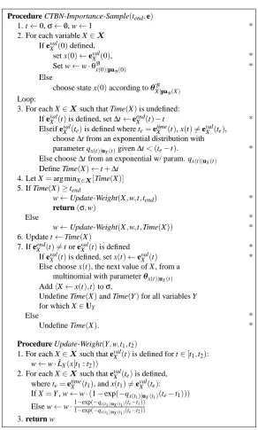
The algorithm for CTBN importance sampling is shown in Figure 4. To more easily describe the evidence, we define a few helper functions:

eval_X (t)is the value of X at time t according to the evidence, or undefined if X has no evidence at t.

etime_X (t)is the first time after t when eval_X (t)is defined.

eend

X (t)is the first time after or equal to t when evalX (t)changes value or becomes undefined.

Note that eend_X (t) =t when there is point evidence at t, when t is the end of an interval of evidence, and

when there is a transition in the evidence at time t.

The line numbers follow those given in the forward sampling algorithm with new or changed lines marked with an asterisk. Time(X)might be set to the end of an interval of evidence which is not a transition time but simply a time when we need to resample a next potential transition. This means that we will not updateσ with a new transition every time through the loop. The algorithm differs from the forward sampling procedure as follows. Step 2 now accounts for evidence at the beginning of the trajectory (using standard likelihood weighting for Bayesian networks). In Step 3, we draw∆t from the truncated exponential if the current value

disagrees with upcoming evidence. If the current evidence includes this variable,∆t is set to the duration of

such evidence. Step 5 updates the weights using the procedure Update-Weight. Finally, Step 7 now deals with variables that are just leaving the evidence set.

3.6 Predictive Lookahead

The algorithm in Figure 4 draws the next state for a variable from the same distribution as the forward sampling algorithm. This may cause a variable to transition several times in a short interval before evidence as the variable “searches” to find a way to transition into the evidence. Thus, we may generate many unlikely samples, making the algorithm inefficient. We can help mitigate this problem by trying to force the variable into a state that will lead to the evidence.

When sampling the next state for variable X at time t, instead of sampling from the multinomial according toθ_x(t)|u

X(t), we would like to sample from the distribution of the next state conditioned on the upcoming evidence. Suppose X is in state xiat time t, and the next evidence for X is state xkat te. Assuming the parents of X do not change before teand ignoring evidence over the children of X , the distribution of the state of X at t given only the evidence can be calculated using Equation 3:

˜

P(Xt+∆t=xj|X[t : t+∆t) =xi,Xte=xk) = 1

Z1

⊤

jQXexp(QX(te−t))1k=pi,j

where 1jis the vector of zeros, except for a one in position j. We can therefore select our new state according to the distribution of ˜P(Xt+∆t|X[t : t+∆t) =xi,Xte =xk)and, assuming state xj is selected, multiply the

weight by θxix j_p|uX(t)

i,j to account for the difference between the target and sampling distributions.

3.7 Particle Filtering

Procedure CTBN-Importance-Sample(tend,e)

1. t←0,σ←/0, w←1 *

2. For each variable X∈X

If eval_X (0)defined,

set x(0)←eval_X (0), *

Set w←w·θBx(0)|pa_B(0) *

Else

choose state x(0)according toθB

X|pa_B(X)

Loop:

3. For each X∈X_{such that Time(X)is undefined:}

If eval_X (t)is defined, set∆t←eend_X (t)−t * Elseif eval_X (te)is defined where te=etimeX (t), x(t)6=evalX (te),

choose∆t from an exponential distribution with

parameter q_x(t)|uX(t)given∆t<(te−t). * Else choose∆t from an exponential w/ param. qx(t)|uX(t)

Define Time(X)←t+∆t

4. Let X=arg minX∈X[Time(X)]

5. If Time(X)≥tend

w←Update-Weight(X,w,t,tend) * return(σ,w)

Else *

w←Update-Weight(X,w,t,Time(X)) * 6. Update t←Time(X)

7. If eend_X (t)6=t or eval_X (t)is defined * If eval_X (t)is defined, set x(t)←eval_X (t) * Else choose x(t), the next value of X , from a

multinomial with parameterθ_x(t)|u

X(t)

AddhX←x(t),titoσ.

Undefine Time(X)and Time(Y)for all variables Y for which X∈UY

Else *

Undefine Time(X). *

Procedure Update-Weight(Y,w,t1,t2)

1. For each X∈Xsuch that eval_X (t)is defined for t∈[t1,t2):

w←w·˜LX(x[t1: t2)) 2. For each X∈X_{such that e}val

X (te)is defined, where te=etime_X (t1), and x(t1)6=evalX (te): If X=Y , w←w·(1−exp(−qx(t1)|uX(t1)(te−t1)))

Else w←w·1−exp(−qx(_t1)|uX(_t1)(te−t1))

1−exp(−qx(t1)|uX(t1)(te−t2))

3. return w

Figure 4: Importance sampling for CTBNs. Changes from Figure 2 are noted with asterisks.

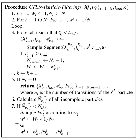
Procedure CTBN-Particle-Filtering({X₀i,wi0}i=1...N,tend,e) 1. k←0,Wt←1,Nr←N

2. For i←1 to N: Pai₀←i, wi←1/N

Loop:

3. For each i such that t_ki<tend:

(X_ki₊₁,t_ki₊₁,wi_k+1)←

Sample-Segment(XPa i k

k ,t Pai

k

k ,wi,tend,e) If t_ki₊₁≥tend

Nremain←Nr−1,

Wt←Wt−wik+1 4. k←k+1

5. If Nr=0 return{Xmii,t

i mi,w

i mi,Pa

i

mi}i=1...N,mi=1...ni,

where niis the number of transitions of the ithparticle 6. CalculateNde f f of all incomplete particles

7. IfNde f f<Nthr

Sample Pai_kaccording to wi_k

wi←Wt×1/Nr Else

wi←wi_k, Pai_k←Pai_k−1

Figure 5: Particle Filtering for CTBNs

At a high level, these methods re-apportion our samples to focus more efforts on more relevant samples— those with higher weights.

The application of this idea to our setting introduces some subtleties because different samples are not generally synchronized. We could pick a time t and run the algorithm in Figure 4 with tend=t so that samples are synchronized at t. We would re-apportion the weights and continue each trajectory from its state at t, first setting Time(X)to be undefined for all X . However, choosing the proper synchronization time t is a non-trivial problem which may depend on the evidence and the speed the system evolves.

Instead of synchronizing all the particles by the time, we can align particles by the number of transitions. If we let tibe the ithtransition time and Xibe the value of X from ti−1to ti, the following recursion holds.

P(X[0 : tn)) =P(X1:n,t1:n,e[0:tn))

=P(X1:n−1,t1:n−1,e[0:tn−1))P(Xn|Xn−1)P(X[tn−1,tn),e[tn−1,tn)|Xn−1,etn−1).

The weighted approximation of this probability is given by

P(X[0 : tn))≈ N

∑

i=1

w(Xi_{[0 : t}

n))δ(X[0 : tn),Xi[0 : tn))

where Xi_{[0 : t}

n)is the ith sample and w(Xi[0 : tn))is the normalized weight of the ithsample. According to Equation 8, the weight can be updated after every transition step. The weight update equation can be shown as

w(Xi[0 : tn))∝w(Xi[0 : tn−1))

˜LX(Xi[tn−1: tn)) ˜L′

X(Xi[tn−1: tn))

.

Thus, to sample multiple trajectories in parallel, we apply the CTBN importance sampling algorithm to each trajectory until a transition occurs. To avoid the degeneracy of the weights, we resample the particles when the estimated effective sample sizeNde f f=_∑ 1

i(wik)2

is below a threshold Nthr. This procedure is similar

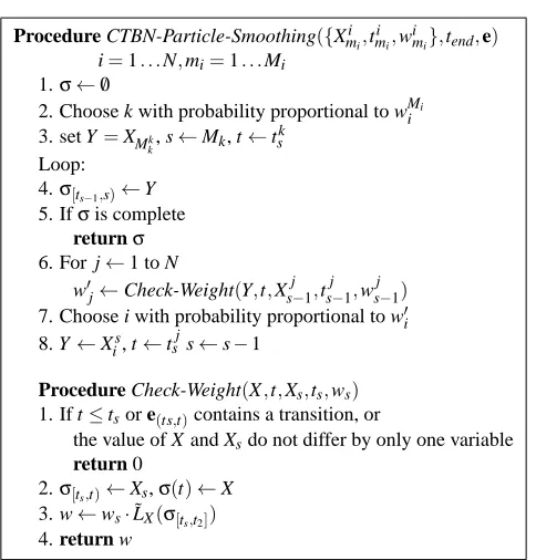
Procedure CTBN-Particle-Smoothing({Xmii,t

i mi,w

i

mi},tend,e) i=1. . .N,mi=1. . .Mi

1.σ←/0

2. Choose k with probability proportional to wMi

i 3. set Y =X_Mk

k, s←Mk, t←t

k s Loop:

4.σ_[ts−1,s)←Y

5. Ifσis complete returnσ 6. For j←1 to N

w′_j←Check-Weight(Y,t,X_sj₋₁,t_sj₋₁,w_sj₋₁)

7. Choose i with probability proportional to w′_i 8. Y←Xs

i, t←t j

s s←s−1

Procedure Check-Weight(X,t,Xs,ts,ws) 1. If t≤tsor e(ts,t)contains a transition, or

the value of X and Xsdo not differ by only one variable return 0

2.σ_[ts,t)←Xs,σ(t)←X

3. w←ws·˜LX(σ[ts,t2])

4. return w

Figure 6: Particle Smoothing for CTBNs

of transitions. To answer queries in the time interval[0,T), we propagate the particles until all of their last transitions are greater than T .

Figure 5 shows the algorithm for generating N trajectories from 0 to T in a CTBN. It assumes that the initial values and the weights have already been sampled. The procedure Sample-Segment loops from line 3 to 7 in Figure 4 until a transition occurs, returns the transition time and variables value, and updates the corresponding weight for that segment. Note that we are approximating the distribution P(X1:n,t1:n,e[0:tn))for all possible n. Therefore, we only propagate and re-apportion weights for particles that have not yet reached time T . Particles that have been sampled past T are left untouched.

3.8 Particle Smoothing

Although the resampling step in the particle filtering algorithm reduces the skew of the weights, it leads to another problem: the diversity of the trajectories is also reduced since particles with higher weights are likely to be duplicated multiple times in the resampling step. Many trajectories share the same ancestor after the filtering procedure. A Monte Carlo smoothing algorithm using backward simulation addresses this problem (Godsill et al., 2004).

The smoothing algorithm for discrete-time systems generates trajectories using N weighted particles

{xi_t,wi_t} from the particle filtering algorithm. It starts with the particles at time T , moves backward one step each iteration and samples a particle according to the product of its weight and the probability of it tran-sitioning to the previously sampled particle. Specifically, in the first step, it samples_exT from particles xiT at time T with probability wi

T. In the backward smoothing steps it samplesextaccording to w_ti_|t+1=wtif(xet+1|xit), where f(ext+1|xit)is the probability that the particle transitions from state xtitoext+1. The resulting trajectory set is an approximation of P(x1:T|y1:T)where y1:Tis the observation.

Joint Pain Barometer

Hungry Eating

Uptake

Full Stomach

Concentration

Drowsy

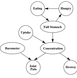
Figure 7: Drug Effect Network

used at the beginning steps of the backward smoothing since the trajectories do not have exactly the same number of transitions, and not all particles at step n can be considered as candidates to move backward. A particle_{Xi

n,tni,wni}is a valid candidate as the predecessor for{Xen+1,etn+1}only if (1) tni<etn+1, (2) the values of X_ni andXen+1differ in only one variable (thus a single transition is possible), and (3) e(ti

n,etn+1)contains no transitions.

Figure 6 shows the smoothing algorithm which generates a trajectory from the filtering particles. We apply the algorithm N times to sample N trajectories. These equally weighted trajectories can be used to approximate the smoothing distribution P(X_[0,T)|e). Generating one trajectory with this smoothing process requires considering all the particles at each step. The running time of sampling N trajectories using particle smoothing is N times of that of particle filtering.

4. Experimental Results

In this section, we report on the performance of our algorithm on synthetic networks and a network built from a real data set of people’s life histories. We tested our algorithm’s accuracy for the task of inference and parameter estimation. We also compare our algorithms with other approximate inference algorithms for CTBNs: the method based on the expectation propagation in Saria et al. (2007) and the method based on Gibbs sampling in El-Hay et al. (2008).

All the algorithms we used in the experiments were implemented in the same code base to make fair comparisons. We tried our best to optimize all the code. The implementations are general so that they can be applied to any CTBN model. Our implementation of EP is adapted from that of Saria et al. (2007) who were kind enough to share their code. The code base is described in Shelton et al. (2010) and is available from the authors’ website.

4.1 Networks

In our experiments, different types of network structures were used, including the drug effect network (Nodel-man et al., 2002), a chain-structured network, and the BHPS network (Nodel(Nodel-man et al., 2005b). All the net-works are at the upper size limit for the exact inference algorithm so that we can compare our result to the true value.

Drug Effect Network: The drug effect network is a toy model of the effect of a pain-relief medicine.

H_E

HC HS

HM Smoking

Married Employ

Children

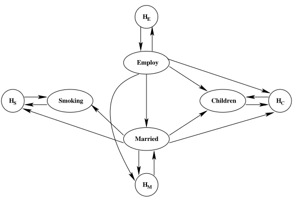
Figure 8: British Household Panel Survey Network

Chain Structured Network: The chain network contains five nodes X0, . . . ,X5, where Xi is the parent of Xi+1for i<5. Each node has five states, s0, . . . ,s4. X0(usually) cycles in two loops: s0→s1→s3→s0 and s0→s2→s4→s0. All the other nodes stay at their current state if it matches their parent and otherwise transition to their parent’s state with a high probability. Each variable starts in state s0.

More specifically, the intensity matrix of X0is

QX0=      

−2.02 1 1 0.01 0.01

0.01 ₋2.03 0.01 2 0.01

0.01 0.01 ₋2.03 0.01 2

2 0.01 0.01 ₋2.03 0.01

2 0.01 0.01 0.01 ₋2.03

     .

For all other nodes, the off-diagonal elements of the intensity matrices are given by

q_s

i,sj|u=sk= (

0.1 if i₆=j and j₆=k,

10 if i₆=j and j=k.

BHPS Network: This network was learned from the British Household Panel Survey (BHPS) (ESRC

Research Centre on Micro-social Change, 2003) data set. The data set provides information about British citizens. The data are collected yearly by asking thousands of households questions such as household or-ganization, employment, income, wealth and health. Similar to Nodelman et al. (2005b), we keep a small set of variables so that exact inference could be applied. We chose four variables: employ (ternary: student, employed, unemployed), children (ternary: 0, 1, 2+), married (binary: not married, married), and smoking (binary: non-smoker, smoker), and we assumed there is a hidden variable (binary) for each of those four variables. We trained the network on 8935 trajectories of people’s life histories. We applied the structural EM algorithm in Nodelman et al. (2005b) and learned the structure of the network shown in Figure 8. We then estimated the parameters of the network using the EM algorithm and exact inference. We consider the learned model as the true BHPS network model for these experiments.

4.2 Evaluation Method

102 103 104 105 10−4

10−3 10−2 10−1

Number of Samples

Relative Bias

non−predict predict

102 103 104 105

10−2 10−1 100

Number of Samples

Relative Standard Deviation

non−predict predict

O( M −1/2)

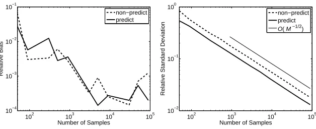
Figure 9: Relative bias and standard deviation of sampling with and without predictive lookahead.

In the inference task, each evidence is a partially observed trajectory of the CTBN network. The evidence is generated using two methods. The first method is to set it manually. The second is to generate a trajectory using the forward sampling algorithm and randomly remove some parts of the sampled trajectory. In particu-lar, we repeated the following procedure n times: for each variable, we randomly removed the information of the trajectory from tsto ts+γT , where T is the total length of the trajectory, tsis randomly sampled from the

[0,T₋γT]uniform distribution andγ<1. After we run the removing procedure n times, there are at most nγ time units of information missing for each variable. In all comparisons, this procedure was applied once and the same evidence was given to all algorithms.

In our experiments, we set our query to be one of three types: the expected total amount of time a variable

X stays on some state xi, the expected total number of times that a variable transitions from state xito state

xj, or the distribution of variable at time t.

For each query, we ran the sampling based algorithms with different sample sizes, M. For each sample size, we ran the experiment N times. We calculated our query according to Equation 6 and compared the result to the true value calculated using exact inference. We used two metrics: the relative bias |∑vM−v∗|

v∗N ,

where vM is the query value of sampling algorithm with sample size M, and v∗is the true value; and the relative standard deviation σM

v∗ where σM is the standard deviation from the true value when sample size is

M. For each sample size, we also recorded the average running time ¯tM of each experiment and used ¯tMto evaluate the efficiency of the algorithm.

In the learning task, we used the sampling algorithms to estimate the parameters of a CTBN network given some partially observed data. Monte Carlo EM (Wei and Tanner, 1990) was applied in this task: In each iteration, we used the sampling based algorithm to estimate the expected sufficient statistics given the incomplete data and used Equation 4 to compute the parameters.

The training data were generated by sampling trajectories from the true model and randomly removing some portion of the information as described above. We sampled another set of trajectories from the true model as the testing data. We calculated the log-likelihood of the testing data under the learned model to evaluate the learning accuracy.

4.3 Inference Experimental Results

In this section, we evaluate the performance of our importance sampling based algorithms in answering queries and compare with the EP algorithm in Saria et al. (2007) and the Gibbs sampling algorithm in El-Hay et al. (2008).

4.3.1 COMPARISON OFIMPORTANCESAMPLING ANDPREDICTIVELOOKAHEAD