Sparse Online Learning via Truncated Gradient
John Langford [email protected]
Yahoo! Research New York, NY, USA
Lihong Li [email protected]
Department of Computer Science Rutgers University
Piscataway, NJ, USA
Tong Zhang∗ [email protected]
Department of Statistics Rutgers University Piscataway, NJ, USA
Editor: Manfred Warmuth
Abstract
We propose a general method called truncated gradient to induce sparsity in the weights of online-learning algorithms with convex loss functions. This method has several essential properties:
1. The degree of sparsity is continuous—a parameter controls the rate of sparsification from no sparsifi-cation to total sparsifisparsifi-cation.
2. The approach is theoretically motivated, and an instance of it can be regarded as an online counterpart of the popular L1-regularization method in the batch setting. We prove that small rates of sparsification result in only small additional regret with respect to typical online-learning guarantees.
3. The approach works well empirically.
We apply the approach to several data sets and find for data sets with large numbers of features, substantial sparsity is discoverable.
Keywords: truncated gradient, stochastic gradient descent, online learning, sparsity, regulariza-tion, Lasso
1. Introduction
We are concerned with machine learning over large data sets. As an example, the largest data set
we use here has over 107sparse examples and 109 features using about 1011 bytes. In this setting,
many common approaches fail, simply because they cannot load the data set into memory or they are not sufficiently efficient. There are roughly two classes of approaches which can work:
1. Parallelize a batch-learning algorithm over many machines (e.g., Chu et al., 2008).
2. Stream the examples to an online-learning algorithm (e.g., Littlestone, 1988; Littlestone et al., 1995; Cesa-Bianchi et al., 1996; Kivinen and Warmuth, 1997).
This paper focuses on the second approach.
Typical online-learning algorithms have at least one weight for every feature, which is too much in some applications for a couple reasons:
1. Space constraints. If the state of the online-learning algorithm overflows RAM it can not efficiently run. A similar problem occurs if the state overflows the L2 cache.
2. Test-time constraints on computation. Substantially reducing the number of features can yield substantial improvements in the computational time required to evaluate a new sample.
This paper addresses the problem of inducing sparsity in learned weights while using an online-learning algorithm. There are several ways to do this wrong for our problem. For example:
1. Simply adding L1-regularization to the gradient of an online weight update doesn’t work
because gradients don’t induce sparsity. The essential difficulty is that a gradient update has
the form a+b where a and b are two floats. Very few float pairs add to 0 (or any other default
value) so there is little reason to expect a gradient update to accidentally produce sparsity.
2. Simply rounding weights to 0 is problematic because a weight may be small due to being useless or small because it has been updated only once (either at the beginning of training or because the set of features appearing is also sparse). Rounding techniques can also play havoc with standard online-learning guarantees.
3. Black-box wrapper approaches which eliminate features and test the impact of the elimination are not efficient enough. These approaches typically run an algorithm many times which is particularly undesirable with large data sets.
1.1 What Others Do
In the literature, the Lasso algorithm (Tibshirani, 1996) is commonly used to achieve sparsity for
linear regression using L1-regularization. This algorithm does not work automatically in an online
fashion. There are two formulations of L1-regularization. Consider a loss function L(w,zi)which is
convex in w, where zi= (xi,yi)is an input/output pair. One is the convex constraint formulation
ˆ
w=arg min
w n
∑
i=1
L(w,zi) subject tokwk1≤s, (1)
where s is a tunable parameter. The other is the soft regularization formulation, where
ˆ
w=arg min
w n
∑
i=1
L(w,zi) +gkwk1. (2)
With appropriately chosen g, the two formulations are equivalent. The convex constraint formu-lation has a simple online version using the projection idea of Zinkevich (2003), which requires
the projection of weight w into an L1-ball at every online step. This operation is difficult to
imple-ment efficiently for large-scale data with many features even if all examples have sparse features although recent progress was made (Duchi et al., 2008) to reduce the amortized time complexity to
the dimension of xi). In contrast, the soft-regularization method is efficient for a batch setting (Lee
et al., 2007) so we pursue it here in an online setting where we develop an algorithm whose com-plexity is linear in k but independent of d; these algorithms are therefore more efficient in problems where d is prohibitively large.
More recently, Duchi and Singer (2008) propose a framework for empirical risk minimization
with regularization called Forward Looking Subgradients, or FOLOSin short. The basic idea is to
solve a regularized optimization problem after every gradient-descent step. This family of algo-rithms allow general convex regularization function, and reproduce a special case of the truncated
gradient algorithm we will introduce in Section 3.3 (withθset to∞) when L1-regularization is used.
The Forgetron algorithm (Dekel et al., 2006) is an online-learning algorithm that manages mem-ory use. It operates by decaying the weights on previous examples and then rounding these weights to zero when they become small. The Forgetron is stated for kernelized online algorithms, while we are concerned with the simpler linear setting. When applied to a linear kernel, the Forgetron is not computationally or space competitive with approaches operating directly on feature weights.
A different, Bayesian approach to learning sparse linear classifiers is taken by Balakrishnan and Madigan (2008). Specifically, their algorithms approximate the posterior by a Gaussian distribution,
and hence need to store second-order covariance statistics which require O(d2)space and time per
online step. In contrast, our approach is much more efficient, requiring only O(d)space and O(k)
time at every online step.
After completing the paper, we learned that Carpenter (2008) independently developed an algo-rithm similar to ours.
1.2 What We Do
We pursue an algorithmic strategy which can be understood as an online version of an efficient L1
loss optimization approach (Lee et al., 2007). At a high level, our approach works with the soft-regularization formulation (2) and decays the weight to a default value after every online stochastic gradient step. This simple approach enjoys minimal time complexity (which is linear in k and in-dependent of d) as well as strong performance guarantee, as discussed in Sections 3 and 5. For instance, the algorithm never performs much worse than a standard online-learning algorithm, and the additional loss due to sparsification is controlled continuously with a single real-valued param-eter. The theory gives a family of algorithms with convex loss functions for inducing sparsity—one per online-learning algorithm. We instantiate this for square loss and show how an efficient
imple-mentation can take advantage of sparse examples in Section 4. In addition to the L1-regularization
formulation (2), the family of algorithms we consider also include some non-convex sparsification techniques.
As mentioned in the introduction, we are mainly interested in sparse online methods for large scale problems with sparse features. For such problems, our algorithm should satisfy the following requirements:
• The algorithm should be computationally efficient: the number of operations per online step
should be linear in the number of nonzero features, and independent of the total number of features.
• The algorithm should be memory efficient: it needs to maintain a list of active features, and
Our solution, referred to as truncated gradient, is a simple modification of the standard stochastic gradient rule. It is defined in (6) as an improvement over simpler ideas such as rounding and
sub-gradient method with L1-regularization. The implementation details, showing our methods satisfy
the above requirements, are provided in Section 5.
Theoretical results stating how much sparsity is achieved using this method generally require additional assumptions which may or may not be met in practice. Consequently, we rely on experi-ments in Section 6 to show our method achieves good sparsity practice. We compare our approach
to a few others, including L1-regularization on small data, as well as online rounding of coefficients
to zero.
2. Online Learning with Stochastic Gradient Descent
In the setting of standard online learning, we are interested in sequential prediction problems where repeatedly from i=1,2, . . .:
1. An unlabeled example xiarrives.
2. We make a prediction based on existing weights wi∈Rd.
3. We observe yi, let zi= (xi,yi), and incur some known loss L(wi,zi)that is convex in parameter wi.
4. We update weights according to some rule: wi+1← f(wi).
We want to come up with an update rule f , which allows us to bound the sum of losses
t
∑
i=1
L(wi,zi)
as well as achieving sparsity. For this purpose, we start with the standard stochastic gradient descent (SGD) rule, which is of the form:
f(wi) =wi−η∇1L(wi,zi), (3)
where∇1L(a,b)is a sub-gradient of L(a,b)with respect to the first variable a. The parameterη>0 is often referred to as the learning rate. In our analysis, we only consider constant learning rate
with fixedη>0 for simplicity. In theory, it might be desirable to have a decaying learning rateηi
which becomes smaller when i increases to get the so called no-regret bound without knowing T in
advance. However, if T is known in advance, one can select a constantηaccordingly so the regret
vanishes as T →∞. Since our focus is on sparsity, not how to adapt learning rate, for clarity, we use
a constant learning rate in the analysis because it leads to simpler bounds.
T0(x, )
x
-T1(x, ,!)
x !
-!
-Figure 1: Plots for the truncation functions, T0and T1, which are defined in the text.
However, a main drawback of (3) is that it does not achieve sparsity, which we address in this paper. In the literature, the stochastic-gradient descent rule is often referred to as gradient descent (GD). There are other variants, such as exponentiated gradient descent (EG). Since our focus in this paper is sparsity, not GD versus EG, we shall only consider modifications of (3) for simplicity.
3. Sparse Online Learning
In this section, we examine several methods for achieving sparsity in online learning. The first idea is simple coefficient rounding, which is the most natural method. We will then consider another
method which is the online counterpart of L1-regularization in batch learning. Finally, we combine
such two ideas and introduce truncated gradient. As we shall see, all these ideas are closely related.
3.1 Simple Coefficient Rounding
In order to achieve sparsity, the most natural method is to round small coefficients (that are no larger
than a thresholdθ>0) to zero after every K online steps. That is, if i/K is not an integer, we use
the standard GD rule in (3); if i/K is an integer, we modify the rule as:
f(wi) =T0(wi−η∇1L(wi,zi),θ), (4)
where for a vector v= [v1, . . . ,vd]∈Rd, and a scalarθ≥0, T0(v,θ) = [T0(v1,θ), . . . ,T0(vd,θ)], with
T0defined by (cf., Figure 1)
T0(vj,θ) =
(
0 if|vj| ≤θ
vj otherwise
.
That is, we first apply the standard stochastic gradient descent rule, and then round small coefficients to zero.
In general, we should not take K=1, especially whenηis small, since each step modifies wi
by only a small amount. If a coefficient is zero, it remains small after one online update, and the rounding operation pulls it back to zero. Consequently, rounding can be done only after every K steps (with a reasonably large K); in this case, nonzero coefficients have sufficient time to go above
the thresholdθ. However, if K is too large, then in the training stage, we will need to keep many
the training phase. The sensitivity in choosing appropriate K is a main drawback of this method; another drawback is the lack of theoretical guarantee for its online performance.
3.2 A Sub-gradient Algorithm for L1-Regularization
In our experiments, we combine rounding-in-the-end-of-training with a simple online sub-gradient
method for L1-regularization with a regularization parameter g>0:
f(wi) =wi−η∇1L(wi,zi)−ηg sgn(wi), (5)
where for a vector v= [v1, . . . ,vd], sgn(v) = [sgn(v1), . . . ,sgn(vd)], and sgn(vj) =1 when vj >0,
sgn(vj) =−1 when vj<0, and sgn(vj) =0 when vj=0. In the experiments, the online method (5)
plus rounding in the end is used as a simple baseline. This method does not produce sparse weights online. Therefore it does not handle large-scale problems for which we cannot keep all features in memory.
3.3 Truncated Gradient
In order to obtain an online version of the simple rounding rule in (4), we observe that the direct rounding to zero is too aggressive. A less aggressive version is to shrink the coefficient to zero by a smaller amount. We call this idea truncated gradient.
The amount of shrinkage is measured by a gravity parameter gi>0:
f(wi) =T1(wi−η∇1L(wi,zi),ηgi,θ), (6)
where for a vector v= [v1, . . . ,vd]∈Rd, and a scalar g≥0, T1(v,α,θ) = [T1(v1,α,θ), . . . ,T1(vd,α,θ)],
with T1defined by (cf., Figure 1)
T1(vj,α,θ) =
max(0,vj−α) if vj∈[0,θ]
min(0,vj+α) if vj∈[−θ,0]
vj otherwise
.
Again, the truncation can be performed every K online steps. That is, if i/K is not an integer, we
let gi=0; if i/K is an integer, we let gi=Kg for a gravity parameter g>0. This particular choice
is equivalent to (4) when we set g such thatηKg≥θ. This requires a large g whenηis small. In
practice, one should set a small, fixed g, as implied by our regret bound developed later.
In general, the larger the parameters g and θare, the more sparsity is incurred. Due to the
extra truncation T1, this method can lead to sparse solutions, which is confirmed in our experiments
described later. In those experiments, the degree of sparsity discovered varies with the problem.
A special case, which we will try in the experiment, is to let g=θin (6). In this case, we can use
only one parameter g to control sparsity. SinceηKg≪θwhenηK is small, the truncation operation
is less aggressive than the rounding in (4). At first sight, the procedure appears to be an ad-hoc way to fix (4). However, we can establish a regret bound for this method, showing it is theoretically sound.
Settingθ=∞yields another important special case of (6), which becomes
where for a vector v= [v1, . . . ,vd]∈Rd, and a scalar g≥0, T(v,α) = [T(v1,α), . . . ,T(vd,α)], with
T(vj,α) =
(
max(0,vj−α) if vj>0
min(0,vj+α) otherwise
.
The method is a modification of the standard sub-gradient descent method with L1-regularization
given in (5). The parameter gi≥0 controls the sparsity that can be achieved with the algorithm.
Note when gi=0, the update rule is identical to the standard stochastic gradient descent rule. In
general, we may perform a truncation every K steps. That is, if i/K is not an integer, we let gi=0; if
i/K is an integer, we let gi=Kg for a gravity parameter g>0. The reason for doing so (instead of a
constant g) is that we can perform a more aggressive truncation with gravity parameter Kg after each
K steps. This may lead to better sparsity. An alternative way to derive a procedure similar to (7)
is through an application of convex hull projection idea of Zinkevich (2003) to the L1-regularized
loss, as in (5). However, instead of working with the original feature set, we need to consider a
2d-dimensional duplicated feature set[xi,−xi], with the non-negativity constraint wj ≥0 for each
component of j (w will also have dimension 2d in this case). The resulting method is similar to ours, with a similar theoretical guarantee as in Theorem 3.1. The proof presented in this paper is more
specialized to truncated gradient, and directly works with xi instead of augmented data[xi,−xi].
Moreover, our analysis does not require the loss function to have bounded gradient, and thus can directly handle the least squares loss.
The procedure in (7) can be regarded as an online counterpart of L1-regularization in the sense
that it approximately solves an L1-regularization problem in the limit ofη→0. Truncated gradient
for L1-regularization is different from (5), which is a naïve application of stochastic gradient
de-scent rule with an added L1-regularization term. As pointed out in the introduction, the latter fails
because it rarely leads to sparsity. Our theory shows even with sparsification, the prediction perfor-mance is still comparable to standard online-learning algorithms. In the following, we develop a general regret bound for this general method, which also shows how the regret may depend on the sparsification parameter g.
3.4 Regret Analysis
Throughout the paper, we usek · k1 for 1-norm, andk · kfor 2-norm. For reference, we make the
following assumption regarding the loss function:
Assumption 3.1 We assume L(w,z)is convex in w, and there exist non-negative constants A and B such thatk∇1L(w,z)k2≤AL(w,z) +B for all w∈Rd and z∈Rd+1.
For linear prediction problems, we have a general loss function of the form L(w,z) =φ(wTx,y). The
following are some common loss functionsφ(·,·)with corresponding choices of parameters A and
B (which are not unique), under the assumption supxkxk ≤C.
• Logistic:φ(p,y) =ln(1+exp(−py)); A=0 and B=C2. This loss is for binary classification
problems with y∈ {±1}.
• SVM (hinge loss): φ(p,y) =max(0,1−py); A=0 and B =C2. This loss is for binary
classification problems with y∈ {±1}.
• Least squares (square loss):φ(p,y) = (p−y)2; A=4C2and B=0. This loss is for regression
Our main result is Theorem 3.1 which is parameterized by A and B. The proof is left to the appendix. Specializing it to particular losses yields several corollaries. A corollary applicable to the least square loss is given later in Corollary 4.1.
Theorem 3.1 (Sparse Online Regret) Consider sparse online update rule (6) with w1=0 andη>0.
If Assumption 3.1 holds, then for all ¯w∈Rdwe have
1−0.5Aη
T T
∑
i=1
L(wi,zi) + gi
1−0.5Aηkwi+1·I(wi+1≤θ)k1
≤η
2B+
kw¯k2
2ηT +
1
T T
∑
i=1
[L(w¯,zi) +gikw¯·I(wi+1≤θ)k1],
where for vectors v= [v1, . . . ,vd]and v′= [v′1, . . . ,v′d], we let
kv·I(|v′| ≤θ)k1=
d
∑
j=1
|vj|I(|v′j| ≤θ),
where I(·)is the set indicator function.
We state the theorem with a constant learning rate η. As mentioned earlier, it is possible to
obtain a result with variable learning rate whereη=ηi decays as i increases. Although this may
lead to a no-regret bound without knowing T in advance, it introduces extra complexity to the presentation of the main idea. Since our focus is on sparsity rather than adapting learning rate, we do not include such a result for clarity. If T is known in advance, then in the above bound, one can simply takeη=O(1/√T)and the L1-regularized regret is of order O(1/
√
T).
In the above theorem, the right-hand side involves a term gikw¯·I(wi+1 ≤θ)k1 depending on
wi+1which is not easily estimated. To remove this dependency, a trivial upper bound ofθ=∞can
be used, leading to L1 penalty gikw¯k1. In the general case ofθ<∞, we cannot replace wi+1 by
¯
w because the effective regularization condition (as shown on the left-hand side) is the non-convex
penalty gikw·I(|w| ≤θ)k1. Solving such a non-convex formulation is hard both in the online and
batch settings. In general, we only know how to efficiently discover a local minimum which is difficult to characterize. Without a good characterization of the local minimum, it is not possible for us to replace gikw¯·I(wi+1≤θ)k1 on the right-hand side by gikw¯·I(w¯ ≤θ)k1 because such a
formulation implies we can efficiently solve a non-convex problem with a simple online update rule. Still, whenθ<∞, one naturally expects the right-hand side penalty gikw¯·I(wi+1≤θ)k1 is much
smaller than the corresponding L1penalty gikw¯k1, especially when wj has many components close
to 0. Therefore the situation withθ<∞can potentially yield better performance on some data. This
is confirmed in our experiments.
Theorem 3.1 also implies a trade-off between sparsity and regret performance. We may simply
consider the case where gi=g is a constant. When g is small, we have less sparsity but the regret
term gkw¯·I(wi+1≤θ)k1 ≤gkw¯k1 on the right-hand side is also small. When g is large, we are
able to achieve more sparsity but the regret gkw¯·I(wi+1≤θ)k1on the right-hand side also becomes
Now consider the case θ=∞and gi=g. When T →∞, if we letη→0 andηT →∞, then
Theorem 3.1 implies
1
T T
∑
i=1
[L(wi,zi) +gkwik1]≤ inf ¯ w∈Rd
" 1
T T
∑
i=1
L(w¯,zi) +gkw¯k1
#
+o(1).
In other words, if we let L′(w,z) =L(w,z)+gkwk1be the L1-regularized loss, then the L1-regularized
regret is small whenη→0 and T →∞. In particular, if we letη=1/√T , then the theorem implies
the L1-regularized regret is T
∑
i=1
(L(wi,zi) +gkwik1)− T
∑
i=1
(L(w¯,zi) +gkw¯k1)
≤ √
T
2 (B+kw¯k
2)
1+ A
2√T
+ A
2√T
T
∑
i=1
L(w¯,zi) +g T
∑
i=1
(kw¯k1− kwi+1k1)
!
+o(√T),
which is O(√T) for bounded loss function L and weights wi. These observations imply our
pro-cedure can be regarded as the online counterpart of L1-regularization methods. In the stochastic
setting where the examples are drawn iid from some underlying distribution, the sparse online
gra-dient method proposed in this paper solves the L1-regularization problem.
3.5 Stochastic Setting
SGD-based online-learning methods can be used to solve large-scale batch optimization problems, often quite successfully (Shalev-Shwartz et al., 2007; Zhang, 2004). In this setting, we can go through training examples one-by-one in an online fashion, and repeat multiple times over the train-ing data. In this section, we analyze the performance of such a procedure ustrain-ing Theorem 3.1.
To simplify the analysis, instead of assuming we go through the data one by one, we assume each additional data point is drawn from the training data randomly with equal probability. This corresponds to the standard stochastic optimization setting, in which observed samples are iid from some underlying distributions. The following result is a simple consequence of Theorem 3.1. For
simplicity, we only consider the case withθ=∞and constant gravity gi=g.
Theorem 3.2 Consider a set of training data zi= (xi,yi)for i=1, . . . ,n, and let
R(w,g) =1
n n
∑
i=1
L(w,zi) +gkwk1
be the L1-regularized loss over training data. Let ˆw1=w1=0, and define recursively for t=1,2, . . .
wt+1=T(wt−η∇1(wt,zit),gη), wˆt+1=wˆt+
where each it is drawn from{1, . . . ,n}uniformly at random. If Assumption 3.1 holds, then at any time T , the following inequalities are valid for all ¯w∈Rd:
Ei1,...,iT
(1−0.5Aη)R
ˆ
wT, g
1−0.5Aη
≤Ei1,...,iT "
1−0.5Aη
T T
∑
i=1 Rwi, g
1−0.5Aη #
≤η2B+kw¯k
2
2ηT +R(w¯,g). Proof Note the recursion of ˆwt implies
ˆ
wT =
1 T T
∑
t=1 wtfrom telescoping the update rule. Because R(w,g) is convex in w, the first inequality follows
di-rectly from Jensen’s inequality. It remains to prove the second inequality. Theorem 3.1 implies the following:
1−0.5Aη
T T
∑
t=1
L(wt,zit) +
g
1−0.5Aηkwtk1
≤gkw¯k1+
η
2B+
kw¯k2
2ηT +
1
T T
∑
t=1
L(w¯,zit). (8)
Observe that
Eit
L(wt,zit) +
g
1−0.5Aηkwtk1
=R
wt, g
1−0.5Aη
and
gkw¯k1+Ei1,...,iT " 1 T T
∑
t=1L(w¯,zit) #
=R(w¯,g).
The second inequality is obtained by taking the expectation with respect to Ei1,...,iT in (8).
If we letη→0 andηT →∞, the bound in Theorem 3.2 becomes
E[R(wˆT,g)]≤E
" 1
T T
∑
t=1
R(wt,g)
#
≤inf
¯
w R(w¯,g) +o(1).
That is, on average, ˆwT approximately solves the L1-regularization problem
inf w " 1 n n
∑
i=1L(w,zi) +gkwk1
#
.
If we choose a random stopping time T , then the above inequalities says that on average wT also
solves this L1-regularization problem approximately. Therefore in our experiment, we use the last
solution wT instead of the aggregated solution ˆwT. For practice purposes, this is adequate even
though we do not intentionally choose a random stopping time.
Since L1-regularization is frequently used to achieve sparsity in the batch learning setting, the
connection to L1-regularization can be regarded as an alternative justification for the sparse-online
Algorithm 1 Truncated Gradient for Least Squares Inputs:
• thresholdθ≥0
• gravity sequence gi≥0
• learning rateη∈(0,1)
• example oracle
O
initialize weights wj←0 ( j=1, . . . ,d) for trial i=1,2, . . .
1. Acquire an unlabeled example x= [x1,x2, . . . ,xd]from oracle
O
2. forall weights wj ( j=1, . . . ,d)
(a) if wj>0 and wj≤θthen wj←max{wj−giη,0}
(b) elseif wj<0 and wj≥ −θthen wj←min{wj+giη,0}
3. Compute prediction: ˆy=∑jwjxj
4. Acquire the label y from oracle
O
5. Update weights for all features j: wj ←wj+2η(y−yˆ)xj
4. Truncated Gradient for Least Squares
The method in Section 3 can be directly applied to least squares regression. This leads to Algorithm 1 which implements sparsification for square loss according to Equation (6). In the description,
we use superscripted symbol wj to denote the j-th component of vector w (in order to differentiate
from wi, which we have used to denote the i-th weight vector). For clarity, we also drop the index
i from wi. Although we keep the choice of gravity parameters giopen in the algorithm description,
in practice, we only consider the following choice:
gi=
(
Kg if i/K is an integer
0 otherwise .
This may give a more aggressive truncation (thus sparsity) after every K-th iteration. Since we do not have a theorem formalizing how much more sparsity one can gain from this idea, its effect will only be examined empirically in Section 6.
In many online-learning situations (such as web applications), only a small subset of the features have nonzero values for any example x. It is thus desirable to deal with sparsity only in this small subset rather than in all features, while simultaneously inducing sparsity on all feature weights. Moreover, it is important to store only features with non-zero coefficients (if the number of features is too large to be stored in memory, this approach allows us to use a hash table to track only the nonzero coefficients). We describe how this can be implemented efficiently in the next section.
Corollary 4.1 (Sparse Online Square Loss Regret) If there exists C>0 such that for all x,kxk ≤C, then for all ¯w∈Rd, we have
1−2C2η
T T
∑
i=1
(wTi xi−yi)2+ gi
1−2C2ηkwi·I(|wi| ≤θ)k1
≤kw¯k
2
2ηT +
1
T T
∑
i=1
(w¯Txi−yi)2+gi+1kw¯·I(|wi+1| ≤θ)k1
,
where wi= [w1, . . . ,wd]∈Rdis the weight vector used for prediction at the i-th step of Algorithm 1; (xi,yi)is the data point observed at the i-step.
This corollary explicitly states that average square loss incurred by the learner (the left-hand
side) is bounded by the average square loss of the best weight vector ¯w, plus a term related to the
size of ¯w which decays as 1/T and an additive offset controlled by the sparsity thresholdθand the
gravity parameter gi.
5. Efficient Implementation
We altered a standard gradient-descent implementation, VOWPAL WABBIT(Langford et al., 2007),
according to algorithm 1. VOWPALWABBIToptimizes square loss on a linear representation wTx
via gradient descent (3) with a couple caveats:
1. The prediction is normalized by the square root of the number of nonzero entries in a sparse vector, wTx/p
kxk0. This alteration is just a constant rescaling on dense vectors which is
effectively removable by an appropriate rescaling of the learning rate.
2. The prediction is clipped to the interval[0,1], implying the loss function is not square loss for unclipped predictions outside of this dynamic range. Instead the update is a constant value, equivalent to the gradient of a linear loss function.
The learning rate in VOWPAL WABBITis controllable, supporting 1/i decay as well as a constant
learning rate (and rates in-between). The program operates in an entirely online fashion, so the memory footprint is essentially just the weight vector, even when the amount of data is very large.
As mentioned earlier, we would like the algorithm’s computational complexity to depend lin-early on the number of nonzero features of an example, rather than the total number of features. The
approach we took was to store a time-stampτj for each feature j. The time-stamp was initialized
to the index of the example where feature j was nonzero for the first time. During online learning, we simply went through all nonzero features j of example i, and could “simulate” the shrinkage of wj after τ
j in a batch mode. These weights are then updated, and their time stamps are set to
i. This lazy-update idea of delaying the shrinkage calculation until needed is the key to efficient
implementation of truncated gradient. Specifically, instead of using update rule (6) for weight wj,
we shrunk the weights of all nonzero feature j differently by the following:
f(wj) =T1
wj+2η(y−yˆ)xj,
i−τj K
Kηg,θ
,
andτjis updated by
τj←τj+
i−τj K
This lazy-update trick can be applied to the other two algorithms given in Section 3. In the coefficient rounding algorithm (4), for instance, for each nonzero feature j of example i, we can
first perform a regular gradient descent on the square loss, and then do the following: if |wj|is
below the thresholdθand i≥τj+K, we round wj to 0 and setτjto i.
This implementation shows the truncated gradient method satisfies the following requirements needed for solving large scale problems with sparse features.
• The algorithm is computationally efficient: the number of operations per online step is linear
in the number of nonzero features, and independent of the total number of features.
• The algorithm is memory efficient: it maintains a list of active features, and a feature can be
inserted when observed, and deleted when the corresponding weight becomes zero.
If we directly apply the online projection idea of Zinkevich (2003) to solve (1), then in the
up-date rule (7), one has to pick the smallest gi≥0 such thatkwi+1k1≤s. We do not know an efficient
method to find this specific giusing operations independent of the total number of features. A
stan-dard implementation relies on sorting all weights, which requires O(d log d)operations, where d is
the total number of (nonzero) features. This complexity is unacceptable for our purpose. However,
in an important recent work, Duchi et al. (2008) proposed an efficient onlineℓ1-projection method.
The idea is to use a balanced tree to keep track of weights, which allows efficient threshold finding
and tree updates in O(k ln d) operations on average, where k denotes the number of nonzero
coef-ficients in the current training example. Although the algorithm still has weak dependency on d, it is applicable to large-scale practical applications. The theoretical analysis presented in this paper
shows we can obtain a meaningful regret bound by picking an arbitrary gi. This is useful because
the resulting method is much simpler to implement and is computationally more efficient per online step. Moreover, our method allows non-convex updates closely related to the simple coefficient rounding idea. Due to the complexity of implementing the balanced tree strategy in Duchi et al. (2008), we shall not compare to it in this paper and leave it as a future direction. However, we be-lieve the sparsity achieved with their approach should be comparable to the sparsity achieved with our method.
6. Empirical Results
We applied VOWPAL WABBIT with the efficiently implemented sparsify option, as described in
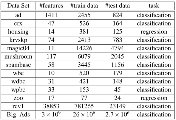
the previous section, to a selection of data sets, including eleven data sets from the UCI repository (Asuncion and Newman, 2007), the much larger data set rcv1 (Lewis et al., 2004), and a private large-scale data set Big_Ads related to ad interest prediction. While UCI data sets are useful for benchmark purposes, rcv1 and Big_Ads are more interesting since they embody real-world data sets with large numbers of features, many of which are less informative for making predictions than others. The data sets are summarized in Table 1.
The UCI data sets used do not have many features so we expect that a large fraction of these features are useful for making predictions. For comparison purposes as well as to better demonstrate the behavior of our algorithm, we also added 1000 random binary features to those data sets. Each
Data Set #features #train data #test data task
ad 1411 2455 824 classification
crx 47 526 164 classification
housing 14 381 125 regression
krvskp 74 2413 783 classification
magic04 11 14226 4794 classification
mushroom 117 6079 2045 classification
spambase 58 3445 1156 classification
wbc 10 520 179 classification
wdbc 31 421 148 classification
wpbc 33 153 45 classification
zoo 17 77 24 regression
rcv1 38853 781265 23149 classification
Big_Ads 3×10⁹ 26×106 2.7×10⁶ classification
Table 1: Data Set Summary.
6.1 Feature Sparsification of Truncated Gradient
In the first set of experiments, we are interested in how much reduction in the number of features is possible without affecting learning performance significantly; specifically, we require the accuracy be reduced by no more than 1% for classification tasks, and the total square loss be increased by no more than 1% for regression tasks. As common practice, we allowed the algorithm to run on the training data set for multiple passes with decaying learning rate. For each data set, we performed 10-fold cross validation over the training set to identify the best set of parameters, including the
learning rateη(ranging from 0.1 to 0.5), the sparsification rate g (ranging from 0 to 0.3), number of
passes of the training set (ranging from 5 to 30), and the decay of learning rate across these passes
(ranging from 0.5 to 0.9). The optimized parameters were used to train VOWPAL WABBITon the
whole training set. Finally, the learned classifier/regressor was evaluated on the test set. We fixed
K=1 andθ=∞, and will study the effects of K andθin later subsections.
Figure 2 shows the fraction of reduced features after sparsification is applied to each data set. For UCI data sets, we also include experiments with 1000 random features added to the original feature set. We do not add random features to rcv1 and Big_Ads since the experiment is not as interesting.
For UCI data sets, with randomly added features, VOWPALWABBITis able to reduce the
num-ber of features by a fraction of more than 90%, except for the ad data set in which only 71% reduc-tion is observed. This less satisfying result might be improved by a more extensive parameter search
in cross validation. However, if we can tolerate 1.3% decrease in accuracy (instead of 1% as for
other data sets) during cross validation, VOWPALWABBITis able to achieve 91.4% reduction,
indi-cating that a large reduction is still possible at the tiny additional cost of 0.3% accuracy loss. With
this slightly more aggressive sparsification, the test-set accuracy drops from 95.9% (when only 1%
loss in accuracy is allowed in cross validation) to 95.4%, while the accuracy without sparsification
Even for the original UCI data sets without artificially added features, VOWPALWABBIT man-ages to filter out some of the less useful features while maintaining the same level of performance.
For example, for the ad data set, a reduction of 83.4% is achieved. Compared to the results above,
it seems the most effective feature reductions occur on data sets with a large number of less useful features, exactly where sparsification is needed.
For rcv1, more than 75% of features are removed after the sparsification process, indicating the effectiveness of our algorithm in real-life problems. We were not able to try many parameters in cross validation because of the size of rcv1. It is expected that more reduction is possible when a more thorough parameter search is performed.
The previous results do not exercise the full power of the approach presented here because the standard Lasso (Tibshirani, 1996) is or may be computationally viable in these data sets. We have also applied this approach to a large non-public data set Big_Ads where the goal is predicting which of two ads was clicked on given context information (the content of ads and query information).
Here, accepting a 0.009 increase in classification error (from error rate 0.329 to error rate 0.338)
allows us to reduce the number of features from about 3×10⁹ to about 24×106, a factor of 125
decrease in the number of features.
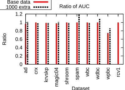
For classification tasks, we also study how our sparsification solution affects AUC (Area Under
the ROC Curve), which is a standard metric for classification.1 Using the same sets of parameters
from 10-fold cross validation described above, we find the criterion is not affected significantly by sparsification and in some cases, they are actually slightly improved. The reason may be that our
sparsification method removed some of the features that could have confused VOWPAL WABBIT.
The ratios of the AUC with and without sparsification for all classification tasks are plotted in Figures 3. Often these ratios are above 98%.
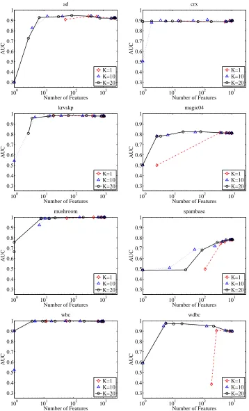
6.2 The Effects of K
As we argued before, using a K value larger than 1 may be desired in truncated gradient and the
rounding algorithms. This advantage is empirically demonstrated here. In particular, we try K=1,
K=10, and K =20 in both algorithms. As before, cross validation is used to select parameters
in the rounding algorithm, including learning rateη, number of passes of data during training, and
learning rate decay over training passes.
Figures 4 and 5 give the AUC vs. number-of-feature plots, where each data point is generated
by running respective algorithm using a different value of g (for truncated gradient) andθ(for the
rounding algorithm). We usedθ=∞in truncated gradient.
The effect of K is large in the rounding algorithm. For instance, in the ad data set the algorithm
using K=1 achieves an AUC of 0.94 with 322 features, while 13 and 7 features are needed using
K=10 and K=20, respectively. However, the same benefits of using a larger K is not observed
in truncated gradient, although the performances with K=10 or 20 are at least as good as those
with K=1 and for the spambase data set further feature reduction is achieved at the same level of
performance, reducing the number of features from 76 (when K =1) to 25 (when K =10 or 20)
with of an AUC of about 0.89.
0 0.2 0.4 0.6 0.8 1
ad crx
housing krvskp magic04 shroom spam
wbc
wdbc wpbc zoo rcv1
Big_Ads
Fraction Left
Dataset Fraction of Features Left Base data
1000 extra
0 0.5 1 1.5 2 2.5 3 3.5 4 4.5 5
ad crx
housing krvskp magic04 shroom spam
wbc wdbc wpbc zoo rcv1
Big_Ads
Fraction Left
Dataset Fraction of Features Left Base data
1000 extra
Figure 2: Plots showing the amount of features left after sparsification using truncated gradient for each data set, when the performance is changed by at most 1% due to sparsification. The solid bar: with the original feature set; the dashed bar: with 1000 random features added to each example. Plot on left: fraction left with respect to the total number of features (original with 1000 artificial features for the dashed bar). Plot on right: fraction left with respect to the original features (not counting the 1000 artificial features in the denominator for the dashed bar).
0 0.2 0.4 0.6 0.8 1 1.2
ad crx
krvskp
magic04 shroom
spam wbc wdbc wpbc rcv1
Ratio
Dataset Ratio of AUC Base data
1000 extra
Figure 3: A plot showing the ratio of the AUC when sparsification is used over the AUC when no sparsification is used. The same process as in Figure 2 is used to determine empirically good parameters. The first result is for the original data set, while the second result is for the modified data set where 1000 random features are added to each example.
6.3 The Effects ofθin Truncated Gradient
In this subsection, we empirically study the effect ofθin truncated gradient. The rounding algorithm
is also included for comparison due to its similarity to truncated gradient whenθ=g. Again, we
used cross validation to choose parameters for eachθvalue tried, and focused on the AUC metric
in the eight UCI classification tasks, except the degenerate one of wpbc. We fixed K=10 in both
100 101 102 103 0.3 0.4 0.5 0.6 0.7 0.8 0.9 1 ad
Number of Features
AUC
K=1 K=10 K=20
100 101 102 103
0.3 0.4 0.5 0.6 0.7 0.8 0.9 1 crx
Number of Features
AUC
K=1 K=10 K=20
100 101 102 103
0.3 0.4 0.5 0.6 0.7 0.8 0.9 1 krvskp
Number of Features
AUC
K=1 K=10 K=20
100 101 102 103
0.3 0.4 0.5 0.6 0.7 0.8 0.9 1 magic04
Number of Features
AUC
K=1 K=10 K=20
100 101 102 103
0.3 0.4 0.5 0.6 0.7 0.8 0.9 1 mushroom
Number of Features
AUC
K=1 K=10 K=20
100 101 102 103
0.3 0.4 0.5 0.6 0.7 0.8 0.9 1 spambase
Number of Features
AUC
K=1 K=10 K=20
100 101 102 103
0.3 0.4 0.5 0.6 0.7 0.8 0.9 1 wbc
Number of Features
AUC
K=1 K=10 K=20
100 101 102 103
0.3 0.4 0.5 0.6 0.7 0.8 0.9 1 wdbc
Number of Features
AUC
K=1 K=10 K=20
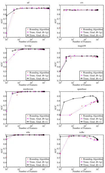
Figure 6 gives the AUC vs. number-of-feature plots, where each data point is generated by
running respective algorithms using a different value of g (for truncated gradient) and θ(for the
rounding algorithm). A few observations are in place. First, the results verify the observation that
the behavior of truncated gradient withθ=g is similar to the rounding algorithm. Second, these
results suggest that, in practice, it may be desirable to useθ=∞in truncated gradient because it
avoids the local-minimum problem.
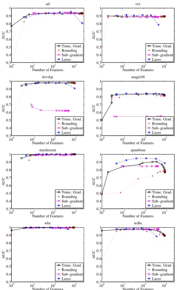
6.4 Comparison to Other Algorithms
The next set of experiments compares truncated gradient to other algorithms regarding their abilities to balance feature sparsification and performance. Again, we focus on the AUC metric in UCI classification tasks except wpdc. The algorithms for comparison include:
• The truncated gradient algorithm: We fixed K=10 and θ=∞, used crossed-validated
pa-rameters, and altered the gravity parameter g.
• The rounding algorithm described in Section 3.1: We fixed K=10, used cross-validated
parameters, and altered the rounding thresholdθ.
• The subgradient algorithm described in Section 3.2: We fixed K=10, used cross-validated
parameters, and altered the regularization parameter g.
• The Lasso (Tibshirani, 1996) for batch L1-regularization: We used a publicly available
imple-mentation (Sjöstrand, 2005).
Note that we do not attempt to compare these algorithms on rcv1 and Big_Ads simply because their sizes are too large for the Lasso.
Figure 7 gives the results. Truncated gradient is consistently competitive with the other two online algorithms and significantly outperformed them in some problems. This suggests the effec-tiveness of truncated gradient.
Second, it is interesting to observe that the qualitative behavior of truncated gradient is often similar to LASSO, especially when very sparse weight vectors are allowed (the left side in the graphs). This is consistent with theorem 3.2 showing the relation between them. However, LASSO usually has worse performance when the allowed number of nonzero weights is set too large (the right side of the graphs). In this case, LASSO seems to overfit, while truncated gradient is more robust to overfitting. The robustness of online learning is often attributed to early stopping, which has been extensively discussed in the literature (e.g., Zhang, 2004).
Finally, it is worth emphasizing that the experiments in this subsection try to shed some light on the relative strengths of these algorithms in terms of feature sparsification. For large data sets such as Big_Ads only truncated gradient, coefficient rounding, and the sub-gradient algorithms are applicable. As we have shown and argued, the rounding algorithm is quite ad hoc and may not work robustly in some problems, and the sub-gradient algorithm does not lead to sparsity in general during training.
7. Conclusion
re-100 101 102 103 0.3 0.4 0.5 0.6 0.7 0.8 0.9 1 ad
Number of Features
AUC
Rounding Algorithm Trunc. Grad. (θ=1g) Trunc. Grad. (θ=∞)
100 101 102 103
0.3 0.4 0.5 0.6 0.7 0.8 0.9 1 crx
Number of Features
AUC
Rounding Algorithm Trunc. Grad. (θ=1g) Trunc. Grad. (θ=∞)
100 101 102 103
0.3 0.4 0.5 0.6 0.7 0.8 0.9 1 krvskp
Number of Features
AUC
Rounding Algorithm Trunc. Grad. (θ=1g) Trunc. Grad. (θ=∞)
100 101 102 103
0.3 0.4 0.5 0.6 0.7 0.8 0.9 1 magic04
Number of Features
AUC
Rounding Algorithm Trunc. Grad. (θ=1g) Trunc. Grad. (θ=∞)
100 101 102 103
0.3 0.4 0.5 0.6 0.7 0.8 0.9 1 mushroom
Number of Features
AUC
Rounding Algorithm Trunc. Grad. (θ=1g) Trunc. Grad. (θ=∞)
100 101 102 103
0.3 0.4 0.5 0.6 0.7 0.8 0.9 1 spambase
Number of Features
AUC
Rounding Algorithm Trunc. Grad. (θ=1g) Trunc. Grad. (θ=∞)
100 101 102 103
0.3 0.4 0.5 0.6 0.7 0.8 0.9 1 wbc
Number of Features
AUC
Rounding Algorithm Trunc. Grad. (θ=1g) Trunc. Grad. (θ=∞)
100 101 102 103
0.3 0.4 0.5 0.6 0.7 0.8 0.9 1 wdbc
Number of Features
AUC
Rounding Algorithm Trunc. Grad. (θ=1g) Trunc. Grad. (θ=∞)
100 101 102 103 0.3 0.4 0.5 0.6 0.7 0.8 0.9 1 ad
Number of Features
AUC
Trunc. Grad. Rounding Sub−gradient Lasso
100 101 102 103
0.3 0.4 0.5 0.6 0.7 0.8 0.9 1 crx
Number of Features
AUC
Trunc. Grad. Rounding Sub−gradient Lasso
100 101 102 103
0.3 0.4 0.5 0.6 0.7 0.8 0.9 1 krvskp
Number of Features
AUC
Trunc. Grad. Rounding Sub−gradient Lasso
100 101 102 103
0.3 0.4 0.5 0.6 0.7 0.8 0.9 1 magic04
Number of Features
AUC
Trunc. Grad. Rounding Sub−gradient Lasso
100 101 102 103
0.3 0.4 0.5 0.6 0.7 0.8 0.9 1 mushroom
Number of Features
AUC
Trunc. Grad. Rounding Sub−gradient Lasso
100 101 102 103
0.3 0.4 0.5 0.6 0.7 0.8 0.9 1 spambase
Number of Features
AUC
Trunc. Grad. Rounding Sub−gradient Lasso
100 101 102 103
0.3 0.4 0.5 0.6 0.7 0.8 0.9 1 wbc
Number of Features
AUC
Trunc. Grad. Rounding Sub−gradient Lasso
100 101 102 103
0.3 0.4 0.5 0.6 0.7 0.8 0.9 1 wdbc
Number of Features
AUC
Trunc. Grad. Rounding Sub−gradient Lasso
gression to the online-learning setting. Theorem 3.1 proves the technique is sound: it never harms performance much compared to standard stochastic gradient descent in adversarial situations. Fur-thermore, we show the asymptotic solution of one instance of the algorithm is essentially equivalent to the Lasso regression, thus justifying the algorithm’s ability to produce sparse weight vectors when the number of features is intractably large.
The theorem is verified experimentally in a number of problems. In some cases, especially for problems with many irrelevant features, this approach achieves a one or two order of magnitude reduction in the number of features.
Acknowledgments
We thank Alex Strehl for discussions and help in developing VOWPAL WABBIT. Part of this work
was done when Lihong Li and Tong Zhang were at Yahoo! Research in 2007.
Appendix A. Proof of Theorem 3.1
The following lemma is the essential step in our analysis.
Lemma 1 Suppose update rule (6) is applied to weight vector w on example z= (x,y)with gravity parameter gi=g, and results in a weight vector w′. If Assumption 3.1 holds, then for all ¯w∈Rd, we have
(1−0.5Aη)L(w,z) +gkw′·I(|w′| ≤θ)k1
≤L(w¯,z) +gkw¯·I(|w′| ≤θ)k1+
η
2B+
kw¯−wk2− kw¯−w′k2
2η .
Proof Consider any target vector ¯w∈Rd and let ˜w=w−η∇1L(w,z). We have w′=T1(w˜,gη,θ). Let
u(w¯,w′) =gkw¯·I(|w′| ≤θ)k1−gkw′·I(|w′| ≤θ)k1.
Then the update equation implies the following:
kw¯−w′k2
≤kw¯−w′k2+kw′−w˜k2
=kw¯−w˜k2−2(w¯−w′)T(w′−w˜)
≤kw¯−w˜k2+2ηu(w¯,w′)
=kw¯−wk2+kw−w˜k2+2(w¯−w)T(w−w˜) +2ηu(w¯,w′) =kw¯−wk2+η2k∇
1L(w,z)k2+2η(w¯−w)T∇1L(w,z) +2ηu(w¯,w′)
≤kw¯−wk2+η2k∇
1L(w,z)k2+2η(L(w¯,z)−L(w,z)) +2ηu(w¯,w′)
≤kw¯−wk2+η2(AL(w,z) +B) +2η(L(w¯,z)−L(w,z)) +2ηu(w¯,w′).
Here, the first and second equalities follow from algebra, and the third from the definition of ˜w.
because w′=T1(w˜,gη,θ), which implies(w′−w˜)Tw′=−gηkw′·I(|w˜| ≤θ)k1=−gηkw′·I(|w′| ≤
θ)k1and|w′j−w˜j| ≤gηI(|w′j| ≤θ). Therefore,
−(w¯−w′)T(w′−w˜) =−w¯T(w′−w˜) +w′T(w′−w˜)
≤
d
∑
j=1
|w¯j||w′j−w˜j|+ (w′−w˜)Tw′
≤gη
d
∑
j=1
|w¯j|I(|w′j| ≤θ) + (w′−w˜)Tw′=ηu(w¯,w′),
where the third inequality follows from the definition of sub-gradient of a convex function, implying
(w¯−w)T∇1L(w,z)≤L(w¯,z)−L(w,z)
for all w and ¯w; the fourth inequality follows from Assumption 3.1. Rearranging the above
inequal-ity leads to the desired bound.
Proof (of Theorem 3.1) Applying Lemma 1 to the update on trial i gives
(1−0.5Aη)L(wi,zi) +gikwi+1·I(|wi+1| ≤θ)k1
≤L(w¯,zi) +k
¯
w−wik2− kw¯−wi+1k2
2η +gikw¯·I(|wi+1| ≤θ)k1+
η
2B.
Now summing over i=1,2, . . . ,T , we obtain
T
∑
i=1
[(1−0.5Aη)L(wi,zi) +gikwi+1·I(|wi+1| ≤θ)k1]
≤
T
∑
i=1
kw¯−wik2− kw¯−wi+1k2
2η +L(w¯,zi) +gikw¯·I(|wi+1| ≤θ)k1+
η
2B
= kw¯−w1k
2− kw¯−w Tk2
2η +
η
2T B+
T
∑
i=1
[L(w¯,zi) +gikw¯·I(|wi+1| ≤θ)k1]
≤ kw¯k
2
2η +
η
2T B+
T
∑
i=1
[L(w¯,zi) +gikw¯·I(|wi+1| ≤θ)k1].
The first equality follows from the telescoping sum and the second inequality follows from the initial condition (all weights are zero) and dropping negative quantities. The theorem follows by dividing with respect to T and rearranging terms.
References
Arthur Asuncion and David J. Newman. UCI machine learning repository, 2007.
University of California, Irvine, School of Information and Computer Sciences,
Suhrid Balakrishnan and David Madigan. Algorithms for sparse linear classifiers in the massive data setting. Journal of Machine Learning Research, 9:313–337, 2008.
Bob Carpenter. Lazy sparse stochastic gradient descent for regularized multinomial logistic regres-sion. Technical report, April 2008.
Nicolò Cesa-Bianchi, Philip M. Long, and Manfred Warmuth. Worst-case quadratic loss bounds for prediction using linear functions and gradient descent. IEEE Transactions on Neural Networks, 7(3):604–619, 1996.
Cheng-Tao Chu, Sang Kyun Kim, Yi-An Lin, YuanYuan Yu, Gary Bradski, Andrew Y. Ng, and Kunle Olukotun. Map-reduce for machine learning on multicore. In Advances in Neural
Infor-mation Processing Systems 20 (NIPS-07), 2008.
Ofer Dekel, Shai Shalev-Schwartz, and Yoram Singer. The Forgetron: A kernel-based perceptron on a fixed budget. In Advances in Neural Information Processing Systems 18 (NIPS-05), pages 259–266, 2006.
John Duchi and Yoram Singer. Online and batch learning using forward looking subgradients. Unpublished manuscript, September 2008.
John Duchi, Shai Shalev-Shwartz, Yoram Singer, and Tushar Chandra. Efficient projections onto
the ℓ1-ball for learning in high dimensions. In Proceedings of the Twenty-Fifth International
Conference on Machine Learning (ICML-08), pages 272–279, 2008.
Jyrki Kivinen and Manfred K. Warmuth. Exponentiated gradient versus gradient descent for linear predictors. Information and Computation, 132(1):1–63, 1997.
John Langford, Lihong Li, and Alexander L. Strehl. Vowpal Wabbit (fast online learning), 2007.
http://hunch.net/∼vw/.
Honglak Lee, Alexis Battle, Rajat Raina, and Andrew Y. Ng. Efficient sparse coding algorithms. In
Advances in Neural Information Processing Systems 19 (NIPS-06), pages 801–808, 2007.
David D. Lewis, Yiming Yang, Tony G. Rose, and Fan Li. RCV1: A new benchmark collection for text categorization research. Journal of Machine Learning Research, 5:361–397, 2004.
Nick Littlestone. Learning quickly when irrelevant attributes abound: A new linear-threshold algo-rithms. Machine Learning, 2(4):285–318, 1988.
Nick Littlestone, Philip M. Long, and Manfred K. Warmuth. On-line learning of linear functions.
Computational Complexity, 5(2):1–23, 1995.
Shai Shalev-Shwartz, Yoram Singer, and Nathan Srebro. Pegasos: Primal Estimated sub-GrAdient SOlver for SVM. In Proceedings of the Twenty-Fourth International Conference on Machine
Learning (ICML-07), 2007.
Robert Tibshirani. Regression shrinkage and selection via the lasso. Journal of the Royal Statistical
Society, B., 58(1):267–288, 1996.
Tong Zhang. Solving large scale linear prediction problems using stochastic gradient descent al-gorithms. In Proceedings of the Twenty-First International Conference on Machine Learning
(ICML-04), pages 919–926, 2004.
Martin Zinkevich. Online convex programming and generalized infinitesimal gradient ascent. In
Proceedings of the Twentieth International Conference on Machine Learning (ICML-03), pages