http://www.sciencepublishinggroup.com/j/fm doi: 10.11648/j.fm.20170306.12
ISSN: 2575-1808 (Print); ISSN: 2575-1816 (Online)
A Study of the Simulation Experiments of Gravity Currents
Yifu Bai
Department of Civil, Environmental and Geomatic Engineering, University College London (UCL), London, United Kingdom
Email address:
To cite this article:
Yifu Bai. A Study of the Simulation Experiments of Gravity Currents. Fluid Mechanics. Vol. 3, No. 6, 2017, pp. 61-65. doi: 10.11648/j.fm.20170306.12
Received: November 1, 2017; Accepted: December 12, 2017; Published: January 8, 2018
Abstract:
Gravity currents which are driven by body gravity forces, occur in the natural environment frequently, such as sea breezes, turbidity currents and avalanches, and sometimes cause natural and environmental disasters around the world. The cause of gravity currents is that the fluid of one density propagates into another fluid of a different density and the motion is largely in the horizontal direction. The objective of this study is to investigate the motion of density driven flows along a horizontal surface and within a stratified fluid, and measure their speeds by the simulation experiments of gravity currents. The speed of the gravity current is constant and able to be calculated with the speed formula. Meanwhile, compare the results with theory for gravity currents and intrusions, estimate theoretical constant parameter and research the behaviour of real fluids. In the experiment, the denser fluid dropped down to the bottom of the tank after the barrier was moved. Next, the fluid moved to the right side of the tank and kept the same shape travelling to the end of the tank. After reaching the end of the tank, the front of the fluid is mixed into the whole fluid. As an inference of this study, it is concluded that the low flow speeds the currents were not influenced by the friction by means of experimental data processing. According to the records of the motion of flows and the behaviour of fluids, the velocity was not constant with distance along the tank due to the human errors of records.Keywords:
Gravity Currents, Density Driven Flows, Fluid Speed, Salt Water1. Introduction
Gravity currents are the kind of density driven flows and turbidity currents are also examples of gravity currents. A turbidity current or density current is a current of rapidly moving, sediment-laden water moving down a slope through air, water, or another fluid. The current moves because it has a higher density than the fluid through which it flows [1, 6]. When the interface is removed, the resulting motion consists of the heavier fluid flowing horizontally beneath the lighter fluid. As the slope of the flow increases, the speed of the current increases. As the speed of the flow increases, turbulence increases, and the current draws up more sediment [2, 5]. The increase in sediment increases the density of the current, and thus its speed, even further. Turbidity currents can reach speeds up to half the speed of sound. Gravity currents are generated when there is a density difference; a two-layer flow is normally created when one density fluid flows into another density fluid, consisting of dense at bottom layer and less dense at top layer [3, 7]. In the experiment, a tank channel was provided and used to measure the dynamics of a two-dimensional gravity current
in a constant cross-section [4]. Two different dense waters with same depth were separated by a barrier in the middle of the channel. When the barrier was removed, the speed of both currents and the shape of the front of both currents were recorded. The motion of the flows and behaviour of fluids were studied.
2. Method of Experiment
1. The tank was filled with water to a depth of 10 cm. A vertical barrier was placed in the middle of the tank to insulate two sides of waters.
2. A bucket of saltwater with 1407.5g of salt in 25 litres of water was provided in the experiment.
3. The first experiment was aiming to achieve a reduced gravity of g’ =1 cm s-2. A pre-calculation was required to calculate the volume of salt water which needed to add into the left hand side of the barrier to create a density difference between two fluids. A red food colouring is also added in the left hand side. The details of the calculation are described in experimental data processing.
right hand side of the barrier. (see the experimental data processing and result descriptions)
5. The vertical barrier is removed, once the motion in the tank was ceased. The location of the fronts were recorded every 10 s and shared in experiment (two layers were recorded, salt water along the bottom and fresh water along the top).
6. The shapes of the front of both currents are recorded and described in the following experimental data processing.
7. Once the currents reach to the end, the water was flushed out. Meanwhile, the data and the mass of salt water after the experiment were recorded and described in data processing. The volume of salt water that needed to add to the next experiment was calculated. (Second experiment should achieve the reduced gravity of g’ = 2 cm s-2. Third experiment should achieve the reduced gravity of g’ = 5 cm s-2.)
8. The experiment was repeated two times to achieve another two different reduced gravity. After the currents reach the far ends of the tank, a barrier was placed 50 cm away from the left end of the tank [8]. The fluids between the left end and the barrier were mixed thoroughly. A blue food colouring was added in this region. After the fluid was ceased in this region, the barrier was removed; the motion and shape of the fluid were recorded and described in the result descriptions.
3. Experimental Data Processing
The volume of salt water, fresh water and mass of salt after measured
Formula: g’ = g (ρ1 – ρ2) / ρ2 Where:
ρ2 = 0.9982 g/cm3 g = 981 mm s-2 ρ1 = 0.9992 g/cm3. For g’ = 1 cm s-2:
1 = 981 (ρ1 – 0.9982)/ 0.9982
ρ1 = 0.9992 g/cm3 From Table 1:
Cs (0.9997-0.9992) / (0.9997-0.9989) = (2-wt.) / (2-1) = 1.4 g/l
Salt needed 1.4 × 60 = 84 g
Volume of solution = 84/ (1407.5/25) = 1.49 l
Volume of Fresh water that add to right side of tank = 1.49 l The theoretical u = c g'H = 1 1×10 = 3.16 cm/s
Find the average speed in the experiment and applying different c value to find the best fit c value [8, 11]. In this experiment, the best estimate of the value of the experimental constant c = 0.4.
Fresh water that measured
The mass of empty bottle measured = 31.97 g The mass of water and bottle = 82.22 g
The mass of fresh sample = 82.22 – 31.97 = 50.25 g Volume of fresh water sample= 50.25/0.9982 = 50.34 cm3 Salt water that measured
The mass of empty bottle measured = 35.92 g The mass of water and bottle = 85.74 g
The mass of salt water sample = 85.74 – 35.92 = 49.82 g Density of salt water sample = 49.82/50.34 = 0.99 g/cm3 % Error = -0.96
The recorded data and calculation for g’ = 1 cm s-2, g’ = 2 cm s-2 and g’ = 5 cm s-2 are shown in Table 2&3.
Table 1. Density and salinity relationship.
NaCl (wt. %) Density (ρ) Cs (g/l)
0.0 0.9982 0.0
0.1 0.9989 1.0
0.2 0.9997 2.0
0.3 1.0004 3.0
0.4 1.0011 4.0
0.5 1.0018 5.0
0.6 1.0025 6.0
0.7 1.0032 7.0
0.8 1.0039 8.1
0.9 1.0046 9.1
1.0 1.0053 10.1
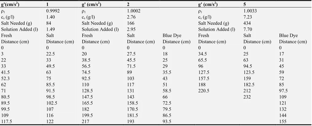
Table 2. Volume of salt water and position of the front of currents in each experiment.
g'(cm/s2) 1 g' (cm/s2) 2 g' (cm/s2) 5
ρ1 0.9992 ρ1 1.0002 ρ1 1.0033
cs (g/l) 1.40 cs (g/l) 2.76 cs (g/l) 7.23
Salt Needed (g) 84 Salt Needed (g) 166 Salt Needed (g) 434 Solution Added (l) 1.49 Solution Added (l) 2.95 Solution Added (l) 7.70
Fresh Salt Fresh Salt Blue Dye Fresh Salt Blue Dye
Distance (cm) Distance (cm) Distance (cm) Distance (cm) Distance (cm) Distance (cm) Distance (cm) Distance (cm)
0 0 0 0 0 0 0 0
3 22.5 20 27.5 18 34.5 25 17
22 33 38.5 45.5 25 65.5 63 31
33 49.5 56.5 71.5 29 96 94.5 45
41.5 63 74.5 89 35.5 127.5 123.5 59
52.3 75 92.5 103 43 157.5 159 72
62 85.5 110 117 51 188 182.5 85
71 91.5 128.5 131 58.5 220.5 212 97.5
80.5 98.5 147.5 143 66 232 109
89.5 102.5 165.5 158.5 72.5 121
99.5 107 182 170.5 79.5 132
109 116 199.5 181.5 86.5 144
g'(cm/s2) 1 g' (cm/s2) 2 g' (cm/s2) 5
127 130.5 233 204 100.5 167
137.5 139.5 215 107 177.5
146.5 147.5 225.5 114.5 190
156.5 153 122.5 201.5
163 162 129.5 213.5
171 171 136 224
186 177.5 143.5 236
194 185 149.5 246
201 191.5 154.5 255
209.5 200 160.5
216.5 208.5 167
223 216 172.5
231 223 177.5
238 229.5 181.5
187 192.5 196.5 202 205.5 209.5 214
Table 3. Theoretical u value (c=1) and percentage of error in each experiment.
g'=1 g'=2 g'=5
Mass of empty bottle (g) 31.97 31.97 31.97 Mass of bottle + fresh sample (g) 82.22 82.22 82.22 Mass of fresh sample (g) 50.25 50.25 50.25 Volume of fresh water sample (cm³) 50.34 50.34 50.34 Mass of empty bottle (g) 35.92 35.92 35.92 Mass of bottle + salt water sample (g) 85.74 85.78 85.96 Mass of salt water sample (g) 49.82 49.86 50.04 Density of salt water sample (g/cm3) 0.99 0.99 0.99
% Error -0.96 -0.98 -0.92
Theoretical u (cm/s) 3.16 4.47 7.07
4. Descriptions of Experimental Result
When the barrier was removed, the denser fluid started to collapse until it reaches to the bottom of the tank, it moved
along the tank to the right (bottom layer of the tank). The less dense fluid flowed to the left direction (the top layer of the tank). The speeds of two fluids were almost same and the shapes of the front of different dense currents that observed in the experiments were almost symmetric. The shape of the front current was presented by the density difference. The section behind the front of the current was unstable. The turbulence behind the front of the current result mixing, the billowing curves along the front became larger, collapsed, and were replaced by the rear current when the size of the billowing current became relatively large [9, 11]. The less dense current moving on the top layer was similar to the denser current, although the colour is difficult to observe
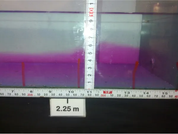
When the currents reached to the ends of the tank, it started to rise a little bit, the rear current was still pushing forward and the section length of the higher front started to increase as shown in Figure 1.
Figure 2. The right end of the blue current with less dense current on the top and denser current on the bottom.
Figure 3. Average speed every 10s in the experiments (y - axis: speed cm/s, x - axis: recoded times).
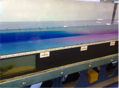
When removing the barrier which 50 cm away to the left, the blue fluid started to rise into the middle layer and moved to the right, the red fluid started to move to the left at the bottom layer as well as the transparent current on the top layer. The shapes of the currents were similar before but the blue current layer was slightly thicker, this could because of the visible colouring make the shape of the current more precise while observing the gravity currents, the blue current slowed down and stopped before reach to the right end [10]. As shown in Figure 2.
5. Conclusion
The Reynolds number is based on the front speed, fluid
depth and coefficient of kinematic viscosity = Uh/ᴠ. In the experiment, the lowest fluid speed was 1.07 cm/s. The fluid depth was 10cm and the kinematic viscosity of water is 0.01 cm2 s-1, so the smallest Reynolds number in the experiments is 1.07 × 10/ 0.01 = 1070 which is bigger than 500. Therefore, the low flow speeds the currents were not affected by the friction. The speeds that recorded every 10s in the experiment are shown in Figure 3. The figure shows that the velocity was not indeed constant with distance along the tank. The lines show that the initial speed were higher than the end speed, this could because of the human error when recording the position of the front current [12].
phenomenon in nature. In avalanches, the denser snow moves at the bottom of surface while the less dense air moves at top. In lava, the high dense lava moves along the surface while the air is less dense compare to lava [13, 14]. Meanwhile, gravity currents are also very common in the built environment. When the door is closed, it separated the air into two rooms with different temperatures, and the higher the temperature of the air has less density compare to the cold air. The cold air will move along the surface of the floor when the door is opened, thus this is experienced that the feet will feel the cold air first when open the door in a warmer room.
References
[1] Rottman, J. W., & Simpson, J. E. (2006). Gravity currents produced by instantaneous releases of a heavy fluid in a rectangular channel. Journal of Fluid Mechanics, 135 (135), 95-110.
[2] Simpson, J. E. (2003). Gravity currents in the laboratory, atmosphere, and ocean. Annual Review of Fluid Mechanics, 14 (1), 213-234.
[3] Bonnecaze, R. T., Huppert, H. E., & Lister, J. R. (1993). Particle-driven gravity currents. Journal of Fluid Mechanics, 250 (-1), 339-369.
[4] Kneller, B. C., Bennett, S. J., & Mccaffrey, W. D. (1999). Velocity structure, turbulence and fluid stresses in experimental gravity currents. Journal of Geophysical Research Oceans, 104 (C3), 5381-5391.
[5] Musuuza, J. L., Attinger, S., & Radu, F. A. (2009). An extended stability criterion for density-driven flows in homogeneous porous media ☆. Advances in Water Resources, 32 (6), 796-808.
[6] Pf, L., & Je, S. (1986). Gravity-driven flows in a turbulent fluid. Journal of Fluid Mechanics, 172 (172), 481-497.
[7] Huppert, H. E., & Woods, A. W. (2006). Gravity-driven flows in porous layers. Journal of Fluid Mechanics, 292 (292), 55-69.
[8] Gladstone, C., & Phillips, J. C. (1998). Experiments on bidisperse, constant-volume gravity currents: propagation and sediment deposition. Sedimentology, 45 (5), 833–843.
[9] Amy, L. A., Hogg, A. J., Peakall, J., & Talling, P. J. (2005). Abrupt transitions in gravity currents. Journal of Geophysical Research Atmospheres, 110 (3), 585-585.
[10] Monaghan, J. J., Cas, R. A. F., Kos, A. M., & Hallworth, M. (1999). Gravity currents descending a ramp in a stratified tank. Journal of Fluid Mechanics, 379 (379), 39-69.
[11] Gladstone, C., Ritchie, L. J., Sparks, R. S. J., & Woods, A. W. (2010). An experimental investigation of density‐stratified inertial gravity currents. Sedimentology, 51 (4), 767-789.
[12] Cantero, M. I., Lee, J. R., Balachandar, S., & Garcia, M. H. (2007). On the front velocity of gravity currents. Journal of Fluid Mechanics, 586 (586), 1-39.
[13] Ungarish, M. (2009). An introduction to gravity currents and intrusions. Crc Press Boca Raton Fl, xviii+489.