Efficient Methods for Robust Classification Under Uncertainty in Kernel Matrices

(1)

Efficient Methods for Robust Classification Under Uncertainty in

Kernel Matrices

Aharon Ben-Tal [email protected]

William Davidson Faculty of Industrial Engineering and Management, Technion- Israel Institute of Technology

Technion City, Haifa 32000, Israel

Sahely Bhadra [email protected]

Chiranjib Bhattacharyya [email protected]

Department of Computer Science and Automation, Indian Institute of Science, Bangalore -560012 Karnataka, India

Arkadi Nemirovski [email protected]

H. Milton Stewart School of Industrial and Systems Engineering Georgia Institute of Technology, Georgia 30332-0205

Atlanta, Georgia, USA

Editor: John Shawe-Taylor

Abstract

In this paper we study the problem of designing SVM classifiers when the kernel matrix, K, is affected by uncertainty. Specifically K is modeled as a positive affine combination of given positive semi definite kernels, with the coefficients ranging in a norm-bounded uncertainty set. We treat the problem using the Robust Optimization methodology. This reduces the uncertain SVM problem into a deterministic conic quadratic problem which can be solved in principle by a polynomial time Interior Point (IP) algorithm. However, for large-scale classification problems, IP methods become intractable and one has to resort to first-order gradient type methods. The strategy we use here is to reformulate the robust counterpart of the uncertain SVM problem as a saddle point problem and employ a special gradient scheme which works directly on the convex-concave saddle function. The algorithm is a simplified version of a general scheme due to Juditski and Nemirovski (2011). It achieves an O(1/T2)reduction of the initial error after T iterations. A comprehensive empirical study on both synthetic data and real-world protein structure data sets show that the proposed formulations achieve the desired robustness, and the saddle point based algorithm outperforms the IP method significantly.

Keywords: robust optimization, uncertain classification, kernel functions

1. Introduction

The Support Vector Machine(SVM) formulation (Vapnik, 1998) learns a classifier of the form

f(x) =sign n

∑

i=1

αiyiK(xi,x) +b

!

(2)

from a training data set D=_{(xi,yi)|xi ∈

X

,yi∈ {1,−1}i=1, . . . ,n}. The coefficients, α, are determined by solving

max

α∈Sn,t

α⊤_e₋1

2t s.t. α⊤Y KYα≤t (2)

where Sn={α|0≤αi≤C,∑ni=1αiyi=0}and Y=diag(y1, . . . ,yn). Each entry of the matrix K, is defined by Ki j =K(xi,xj)where K :

X

×

X

→R, is a kernel function and it defines a dot product in an associated Reproducing Kernel Hilbert Space (Mercer, 1909; Shawe-Taylor and Cristianini, 2000). As a consequence of K(_·,_·) being a dot product, the matrix K needs to be positive semi-definite (see, e.g., Shawe-Taylor and Cristianini, 2000) for any positive integer n.

Observations emanating from real world data are often plagued by uncertainty. The problem of designing classifiers for uncertain observations remain an interesting open problem and has gained considerable interest in the recent past. Previous attempts (Ghaoui et al., 2003; Bhattacharyya et al., 2004; Shivaswamy et al., 2006; Bhadra et al., 2009; Ben-Tal et al., 2011) at designing robust classifiers have been limited to the case of linear classification where the uncertainty is specified over an explicitly stated feature map.

Consider the problem of automated protein structure classification, an important problem of Computational Biology, where no such feature map is available. Protein Structures are specified by a set of 3D coordinates and it is possible to design kernel functions for protein structures based on the coordinates (Qiu et al., 2007; Bhattacharya et al., 2007). Unfortunately the coordinates are not known precisely and this makes the kernel values uncertain. Motivated by this problem (Bhadra et al., 2010) initiated a study of designing robust classifiers when the entries of the kernel matrix are independently distributed random variables (a somewhat problematic assumption). The approach, based on Chance-Constraints (probabilistic) formalism, leads to a non-convex problem which may result in an invalid (i.e., indefinite) kernel matrix.

In this paper we propose a Robust Optimization(RO) approach which overcomes the above drawbacks. The approach employs a geometric description of uncertainty instead of the probabilis-tic description used earlier (Bhadra et al., 2010). The uncertainty in the kernel matrix K is modeled by a bounded convex set, which encompasses several possible realizations of K. This new approach results first in a robust counterpart of the uncertain SVM which can be cast as a Conic Quadratic (CQ) problem. Such problems can be solved in polynomial time by Interior Point (IP) algorithm. However for large-scale problems IP methods become intractable. Our main contribution here is to reformulate the robust counterpart as a saddle point problem. Due to favorable conditions satisfied by the saddle function one can in principle refer to a gradient-based general scheme introduced in (Juditski and Nemirovskii, 2011) for solving such saddle point problems. Using this scheme we propose an algorithm, which has a much more simplified analysis, and achieves the same efficiency estimate, namely it achieves the O(1/T2)reduction in the initial error after T iterations. Experi-mental results performed on synthetic data, as well as real-world protein structure data sets, show that the saddle-point based algorithm outperforms the IP method considerably. We further conduct detailed experimental evaluation to test the robustness and scalability of the obtained classifiers.

(3)

its application to the minimax problem. In Section 6 we prepare the ground for a comprehensive computational study by introducing various prediction rules and related error metrics. The results of the computational study are described in Section 7.

1.1 Notation

The space of symmetric positive semi-definite n_×n matrices will be denoted as

S

₊n. Let A_∗B

denote the the Hadamard prodcuct of two matrices(A_∗B)i j =Ai jBi j where A and B are two square

matrices. Frobenius norm of matrix A will be denoted as_kA_kF =

q

∑i jA2i j. Let 1Abe the indicator function for the event A. The uniform random variate will be represented as U(a,b) (a<b). We denote diag(x1, . . . ,xn)to be a n×n diagonal matrix whose ith diagonal entry is xi.

2. Motivation: Uncertain Kernels and Automated Protein Structure Classification

Classification of protein structures into various classes like families, superfamilies etc remains an important research challenge in computational biology (see Holm and Sander, 1996 for an introduc-tion). Kernel based classifiers are becoming increasingly popular (Qiu et al., 2007; Bhattacharya et al., 2007), for addressing this problem.

Usually a protein structure is specified by the positions of alpha carbon (Cα) atoms. A formal description of Cα atoms and protein structures is beyond the scope of the paper and we refer the reader to Branden and Tooze (1999) for an introduction. In the sequel we will denote protein structure by a set

P=_{ci∈R3|i=1,···,s}, (3) where each Cαatom is determined by spatial coordinates ci={ci1,ci2,ci3}obtained by X-ray crys-tallography. Automated classification of such structures is an extremely useful and challenging problem in computational biology. In the recent past kernel based methods (Qiu et al., 2007; Bhat-tacharya et al., 2007) have emerged as an interesting alternative to this problem.

Biologists often determine the similarity between a pair of structures by first computing an

alignment and then measuring the quality of the alignment by root mean square deviation(RMSD).

We do not formally define the notion of alignment and RMSD in this paper but the refer the in-terested reader to Shindyalov and Bourne (1998) and Holm and Sander (1996) for an introduction. Though computing structural alignment is an intractable problem there are several heuristic algo-rithms like DALI (Holm and Sander, 1996), CE (Shindyalov and Bourne, 1998) etc, which works well in practice. Existing literature (Qiu et al., 2007; Bhattacharya et al., 2007) on kernel design rely on structural alignments computed by such programs.

All such procedures implicitly assume that the protein structures are specified exactly, that is, the location of the atoms constituting the structure is known precisely. Unfortunately in reality, the coordinates, ci, are difficult to determine with exact precision and is highly dependent on the

resolution of X-ray diffraction experiment.1 For a protein structure P, the resolution information

r, specifies the error in each coordinate. More formally the position of the ith atom in a protein

structure P (see (3)) could be anywhere in the uncertainty box_{c_|kc₋¯cik∞≤r},around the value ¯ci. For any r>0 one can now define the uncertainty set U(P)for any P as follows

U(P) =_{R_|R=_{z1, . . . ,zs} kzi−¯cik∞≤r,zi∈R3,i=1, . . . ,s}. (4)

(4)

Figure 1: (a) Pictorial presentation of Cαatoms of protein d1vsra1(top) and d1gefa1(bottom). (b) Structural alignment between them. (c) Possible perturbation within resolution limit. (d) Alignment among perturbed structures

Furthermore we would refer to

¯

P=_{¯ci∈R3|i=1, . . . ,n}

as the nominal structure and U(P)as the uncertainty set associated with it. The set U(P) character-izes all alternative structures, including ¯P for a given value of r.

The structural alignment between P and P′ in presence of uncertainty sets U(P) and U(P′)is not defined anymore. Even when r is small, the alignment scores between two nominal structures,

¯

P and ¯P′ can differ significantly from the alignment scores between an arbitrary R and R′ where

R_∈U(P),R′_∈U(P′). This difference in alignment scores leads to uncertain kernel values.

For example, consider two proteins2 d1vsra1(denote it by P) and d1gefa1(denote it by P′) belonging to protein superfamily Restriction endonuclease-like. The value of r for P is 1.8 ˚A and

for P′it is 2.0 ˚A respectively. The program DALI computes a structural alignment with RMSD of 3.7

˚

A between these two structures. Figure 1(a) shows pictorial presentation of Cαatoms of these two proteins while Figure 1(b) shows structural alignment between them. If one ignores the uncertainty one obtains a kernel value of 1.3585, using the kernel function described in Bhattacharya et al. (2007). On randomly sampled structures, from the corresponding uncertainty box (4) we observe that the kernel value ranged from 1.1542(=Kmin)≤K(P,P′)≤1.4964(=Kmax), see Figure 1(c,d). This variability is indeed substantial. In superfamily Restriction endonuclease-like, more than 60% of the kernel values, computed between any pair of nominal protein structures, lie between

Kminand Kmax.

(5)

This demonstrates that accounting for resolution information leads to considerable uncertainty in kernel values. There is clearly a need for designing classifiers which can withstand this variation in kernel values. This is an extremely challenging problem which has not been well studied in the literature. Recently (Bhadra et al., 2010) initiated a study of this problem in a probabilistic setting. In the following section we review this work, to identify key shortcomings and subsequently propose a robust optimization procedure to address them.

3. Related Work

In Bhadra et al. (2010), the uncertainty is modeled by independent noise in each of the entries of the kernel matrix K. The uncertain event α⊤Y(K)Yα≤t is then required to occur with high probability. This results in the following chance constraint problem:

p∗=max t,α∈Sn

α⊤_e₋1

2t (5)

s.t. Prob

α⊤_Y_(K₊_Z₎_Y_α_≤_t_≥₁₋_ε ₍₆₎

whereε<0.5, and where Z is a random matrix variate.

Problem (5) is hard to solve since typically the feasible set is non-convex. The key result is the derivation of a lower bound on p∗under probabilistic assumptions on the entries of Z

Theorem 1 [Bhadra et al., 2010] Let Z be an n_×n random symmetric matrix with independent entries, Zi j, each having finite support, P(ai j ≤Zi j ≤bi j) =1 and E(Zi j) =0. Then the chance

constraint in (5) is satisfied at any pair(α,t)which is feasible for the constraint

α⊤_{Y KY}_α₊p_{2 log}₍₁_/_ε₎_k_β′_∗₍_Y_αα⊤_Y₎_k F ≤t

whereβ′_{i j} =li jγi jwhere li j= bi j−ai j

2 , ci j=

bi j+ai j

2 , ˆµi j=−

ci j

li j and

andγi j= min{σ≥0|σ

2 2z

2₊_ˆµ

i jz−log(cosh(z) + ˆµi jsinh(z))≥0, ∀z ∈ R}.

Proof See Bhadra et al. (2010).

Theorem 1 is used to replace (5) by the following problem, whose optimal value lower-bounds p∗. Specifically p∗>p, whereˆ

ˆ

p=max t,α∈Sn

1

2t−

∑

_i αi

s.t.

∑

i j

yiyjαiαjKi j+κ

r

∑

i j

βi jα2iα2j≤t (7)

where,κ=p2 log(1/ε)andβi j=β

′₂

i j. Any solution of the above problem is guaranteed to satisfy the chance constraint of problem (5).

(6)

was suggested for solving this problem. In the sequel RSVM will denote the solution of (7) by the Quasi newton procedure. The second most important drawback is that the constraint (6) does not define a valid model of uncertainty.

To constitute a valid characterization of uncertainty set the constraint (6) needs to be modified as follows

Prob

α⊤_Y_(K₊_Z₎_Y_α_≤_t_≥₁₋_ε_, _K₊_Z_∈

_S

+

n

The formulation (5) solves a relaxed version of the above problem by ignoring the psd requirement. As a consequence the resultant optimization problem becomes non-convex. Thirdly, the assumption that entries of Z are independently distributed is extremely unrealistic; often the uncertainty in the entries are due to uncertainty in the observations hence K(xi,xj)is seldom independent of K(xi,xl) for distinct i,j,l.

In this work we pursue a RO methodology where the uncertainty is described by a geometric set. This allows us to alleviate the drawbacks associated with the probabilistic model. In the next section we describe a RO procedure for designing robust classifiers.

4. Affine Uncertainty Set Model for Uncertain Kernel Matrices

In this section we introduce an uncertainty set over psd matrices and study the resultant robust SVM problem using an RO approach.

4.1 Robust Optimization

Consider an uncertain optimization problem (8) where f,gi: S⊂(Rn×Rk)⇒R

min

x∈Rnf(x,Ψ) (8)

gi(x,Ψ)≤0 i=1, . . . ,m

where Ψ_∈Rkis a vector of uncertain parameters. The UOP is in fact a family of problems -one for each realization ofΨ. In the RO framework the information related toΨis modelled as a geometric uncertainty set

E

_⊂_Rkand the family of problems, (8) is replaced by its robust counterpart:

r∗=min

x maxΨ_∈E f(x,Ψ) (9)

gi(x,Ψ)≤0∀Ψ∈

E

i=1, . . . ,m.

A solution of (9) is feasible to (8) for any realization ofΨ_∈

E

and the objective function is guaran-teed to be no worse than r∗. The uncertainty set

E

is typically a polytope or ellipsoid or intersection of such sets. These sets yield useful models of uncertainty, which lead to tractable optimization problems (Ben-Tal et al., 2009). A general representation of

E

is as follows

E

=_{Ψ=_Ψ¯ ₊

∑

L i=1

ηiΨi|kηk ≤ρ}

where ¯Ψis the nominal value of the uncertain vectorΨ, the vectorsΨiare possible scenarios of it, andηis a perturbation vector. The norm is suitably defined to capture the geometry of the set. As an example, Consider the ellipsoidal set

(7)

where Q∈

S

n

+and is positive definite. It is easily seen that the set can be represented by

E

withΨi

being the columns of Q−12 and wherek · kis the L₂norm.

In general the RC of an UOP may have infinite number of constraints and is often NP hard. However in several important cases it reduces to a polynomially solvable convex optimization prob-lem. We refer the reader to Ben-Tal et al. (2009) for a comprehensive treatment of RO problems.

4.2 Affine Uncertainty Set Model

Recall the setup for the problem, there is a black box which when presented with a pair of obser-vations z,z′_∈

X

computes the kernel value K(z,z′). We assume that if z and z′ are noisy obser-vations with uncertainty sets U(z) and U(z′) with nominal values znomand z′nomrespectively then

K(z,z′) =K(znom,z′nom), defines a kernel function and will be called the nominal kernel. The differ-ence between actual and the nominal kernel is expressed by a linear combination of known L kernel functions, Kl,l=1, . . . ,L evaluated at points z,z′, as follows:

K(z,z′)₋K(z,z′) =

L

∑

l=1

ηlKl(z,z′).

When there is no uncertainty K(z,z′) =K(z,z′)andη=0. The value of K(z,z′)lies in the uncer-tainty set

{K(z,z′) +

L

∑

l=1

ηlKl(z,z′)|kηkp≤κ,ηl ≥0∀l=1, . . . ,L} (10)

where_kη_kp,p≥1 denotes the lpnorm onη. The constraintηl ≥0 is needed to ensure that each element in the set represents a valid kernel evaluation. The quantity κ measures the quality of approximation and hence the uncertainty. Ifκ=0 then we have no uncertainty. Asκincreases the uncertainty set increases. In the sequel we will refer to ¯K,Kl as base kernels.

We impose the uncertainty set (10) to all examples of interest which immediately leads to the following model of uncertainty on the kernel matrix corresponding to the training set,

E

(κ) =_{K=K+

L

∑

l=1

ηlKl,kηkp≤κ ηl ≥0,l=1, . . . ,L}. (11)

The matrices K,Kl∈

S

n+are obtained by evaluating the known kernel functions K,Klon the training set. As any K∈

E

(κ) is always positive semi-definite, the set

E

(κ) defines a valid model for describing uncertainty in psd matrices. In a later subsection we will discuss the relevance of this setup to protein structure classification problem.

The Robust SVM problem (2) with uncertain K, as characterized in (11), can now be cast as follows

max

α∈Sn

min

K∈E(κ) −

1 2α

⊤_{Y KY}_α₊_α⊤_e

or more explicitly

max

α∈Sn

min_k_η_k_p_≤_κ ₋1 2α

⊤_{Y KY}_α₋1 2α

⊤_Y

∑

L

l=1

(ηlKl)Yα+α⊤e . (12)

(8)

which occurs atηl=κ aq_l−1 kakqq−1 ≥

0 where_{k · k}qis the dual norm ofk · kp, with q= _p₋p₁for any p>1. For p=1 one needs to observe that optimality is achieved at ηl ≥0. Indeed there exists some l such that al =kak∞. The optimal ηis given by the condition that∑l:al=kak∞ηl=1 andηl ≥0. If

al <kak∞thenηl is strictly 0. At optimalityηl ≥0, and hence the resulant optimal kernel lies in

E

(κ).

Before proceeding further it might be useful to discuss the Computation of b. Recall that one also needs to compute b in (1). The choice of b is governed by the following procedure. For a given

K,K1, . . . ,KLlet the optimal solution of (12) beα∗andη∗. Thisη∗ can be viewed as defining an effective kernel K=K+∑L_l₌₁η∗_lKland hence b can be computed as

b= 1

# SV _j

∑

_∈_SV[yj−

∑

_i yiα ∗

iKi j] SV ={i|αi>0}.

For p=2 the problem (12) can be solved as a Second Order Cone Program(SOCP)3 min

α∈Sn,a,t

1 2t+

1

2α⊤Y KYα−α⊤e (13)

s.t _ka_k2≤t

α⊤_{Y K}

lYα≤al, ∀l=1, . . . ,L.

SOCP problems such as (13) can be solved by Interior point(IP) algorithms (e.g., CPLEX, MOSEK, Sedumi) and will be denoted by Uncertainty-Set SVM ( USSVMSOCP).

Generic IP solvers are inadequate for large scale classification problems. Instead, we demon-strate here that the minimax reformulation, (12), admits algorithms which are better suited to large scale problems. For simplicity of exposition we will consider the case p=2. The results can be easily extended for the general case, p>1. Before we discuss the algorithmic aspects it maybe useful to discuss the computation of the base kernels.

4.3 Evaluation of Base Kernels

Recall that in the protein structure classification problem each observation is specified by a(_P¯_,_U₍_P₎_,_y₎_, where P(see (3)) is the nominal structure, U(P)(see (4)) is the uncertainty set specified by the reso-lution and y is the label. We discuss this problem in a formal setup and motivate the uncertainty set described in (10).

To closely parallel the protein structure classification setting we consider the following setup. Given a data set D=_{(xi,Ui)|xi∈Ui,Ui∈

X

,i=1, . . . ,m}where an observation, xi, is not directly specified, instead a nominal value, xi, and an uncertainty set Uiare given. When there is no uncer-tainty the set Ui reduces to only xi. We are also given a kernel function K :

X

×

X

→R. We make no assumptions about the functional form of K(_·,_·), and we assume that there is a black box which when presented with any pair z,z′_∈

X

returns a value K(z,z′).

Let us now consider the computation of K(xi,xj). Since xi,xjare uncertain the precise value of

K(xi,xj)is not known but it for sure lies in the set

U

(x,x′) =_{K(z,z′)_|z_∈U(x),z′_∈U(x′)_}.

3. This is also true for any(p>1)because any p-norm can be represented by conic quadratic inequalities. For a more

(9)

If there is no uncertainty then the set

U

(x,x′) is a singelton, K(x,x′). However as the functional form of K is not known, it is not clear how to characterize the elements of

U

which is amenable to the RO procedure. We propose to circumvent this problem by building an alternate description of the set

U

using a sampling procedure. We make L independent draws from the uncertainty sets. In the lth draw we obtain Ol =_{zl₁, . . . ,zl_m_} where zl_i is an independent and uniform draw from

Ui. For a given Ol we invoke the kernel function K to obtain an m×m kernel matrix Kl where

Kl(xi,xj) =K(zli,zlj). Once Kl are determined we propose to approximate

U

by uncertainty set described in (10).

5. An Algorithm for a Special Class of Convex-Concave Saddle Point Problems

In this section we describe a novel algorithm, which is essentially a special case of an algorithm presented in Juditski and Nemirovski (2011), for a class of convex-concave saddle point problems. The algorithm is iterative in nature, requires only first order information, and has O(1/T2₎

conver-gence where T is the total number of iterations. The proposed algorithm applies generally, more specifically we show that it can be used to solve (12) and the convex version of (7).

5.1 Assumptions

Let U be a closed convex set in Euclidean space E,_{k · k}be a norm on E, andω(u): U_→R be a

function. We say thatω(_·)is a distance-generating function (d.-g.f.) for U compatible with_{k · k}, if ωis convex and continuous on U , admits a continuous on the set Uo=_{u :∂ω(_·)₆=/0_}selection of ω′₍_u₎_∈_∂ω₍_u₎_{and is strongly convex, modulus 1 w.r.t.}_{k · k}_:

hω′(u)₋ω′(u′),u₋u′_{i ≥ k}u₋u′_k2 _∀u,u′_∈Uo. Assume that

• X is a closed and bounded convex subset in a Euclidean space

X

, and Y is a closed convex subset in a Euclidean space

Y

•

X

,

Y

are equipped with norms_{k · k}X,k · kY, the conjugate norms beingk · kX,∗,k · kY,∗;

• X is equipped with a d.-g.f. ωX(·)compatible withk · kX, and

Y

is equipped with a d.-g.f.

ωY(·). We denote by xωthe minimizer ofωX(·)on X (note that xω∈Xo) and set

ΩX =max

x_∈X ωX(x)−minx_∈XωX(x).

We assume that the minimizer ofωY(·)is the origin in

Y

, and set

ΩY = max

kykY≤1

ωY(y)−min

y∈YωY(y).

We are interested in solving a saddle point problem

SadVal=min

x∈Xmaxy∈Y φ(x,y), (14)

(10)

A.1. φ(x,y): Z :=X×Y→R is continuously differentiable function which is convex in x∈X and

is strongly concave, modulusθ>0 w.r.t._{k · k}Y, in y∈Y , that is,

hφ′y(x,y′)−φ′y(x,y),y−y′i ≥θky−y′k2Y ∀(x∈X,y,y′∈Y).

A.2. ∇φ(_·,_·)is Lipschitz continuous on Z=X_×Y

A.3. φ(x,y)is affine in x:φ(x,y) =_hx,a(y)_i+g(y).

In the sequel, we set

φ(x) =max

y∈Y φ(x,y), φ(y) =minx∈Xφ(x,y),

so thatφis a continuous convex function on X ,φis a continuous strongly concave, modulusθw.r.t.

k · kY, function on Y , and

min

x∈Xφ(x) =SadVal=maxy∈Y φ(y)

and the set of saddle points ofφon X_×Y is X_∗_×{y_∗_}, where X_∗=Argmin_Xφ, and y_∗=Argmax_Yφ. Finally, we denote byεsad(z), z∈Z, the natural saddle point proximity measure:

εsad(x,y) =φ(x)₋φ(y) =hφ(x)₋min X φ

i +

max

Y φ−φ(y)

.

5.2 Fixed Step-size per Stage(FSS) Algorithm for Convex-Concave Saddle Point Problem

The MPb algorithm presented in Juditski and Nemirovski (2011) is an extremely fast algorithm for convex-concave saddle point problems. Computation proceeds in several stages, each stage consisting of multiple updates involving varying stepsizes. Here we introduce a variation of the MPb algorithm called FSS, which employs fixed stepsize at every stage of the algorithm. We prove that this apparent limitation does not harm the theoretical convergence. The proof (see Appendix A) needs milder assumptions and is much simpler than the original MPb algorithm.

We present a variation of the algorithm where the stepsizes are fixed at every stage without any loss of convergence efficency. In the following we present the Fixed stepsize per stage(FSS) version of the MPb algorithm along with convergence analysis.

5.2.1 FSS ALGORITHM

We begin by introducing some notation

G(x,y) =

Gx(x,y):=∂φ

(x,y)

∂x =a(y); Gy(x,y):=−

∂φ(x,y)

∂y

: Z :=X_×Y _→

Z

:=

X

_×

Y

be the monotone operator associated with the saddle point problem (14). By A.1, this operator is Lipschitz continuous, and, as we see, its x-component depends solely on y. As a result, we can specify the partial Lipschitz constants Lxy,Lyysuch that

∀(x,x′∈X,y,y′∈Y):

kGx(x,y)−Gx(x,y′)kX,∗≤Lxyky−y′kY;kGy(x,y)−Gy(x′,y)kY,∗≤Lxykx−x′kX; kGy(x,y)−Gy(x,y′)kY,∗≤Lyyky−y′kY.

(11)

We are now ready to present FSS algorithm. Execution of the algorithm is split intostages. At the beginning of stage s=0,1, ...we have at our disposal positive Rsand a point ¯ys∈Y such that

ky¯s−y_∗kY ≤Rs/2. (Is)

These data define the quantities

(a) Zs={(x; y)∈Z :ky−y¯skY ≤Rs},

(b)

L

_s=2Lxy

p_Ω

XΩYRs+LyyΩYR2s,τs=1/

L

s

(c) αs= [Lxy

p_Ω

XΩYRs]/

L

s,βs= [Lxy

p_Ω

XΩYRs+LyyΩYR2_s]/

L

s=1−αs,

(d) ωs(x,y) =

h αs

ΩXωX(x) +

βs

ΩYωY([y−y¯s]/Rs)

i ,

(e) Ns=Ceil

64Lxy√ΩXΩYR−s1+32LyyΩY

θ

.

(16)

At stage s we carry out Nssteps of the following recurrence:

1. Initialization: We set z1,s= (xω,y¯s) =argminZωs(·). 2. Step t=1,2, ...,Ns: Given zt,s∈Zo, we compute

wt,s = argminu∈Z

hτsG(zt,s)−ω′s(zt,s),ui+ωs(u)

zt+1,s = argminu∈Z

hτsG(wt,s)−ω′s(zt,s),ui+ωs(u) (17)

and pass to step t+1, provided t<Ns. When t =Ns, we define the approximate solution to (14) built in course of s stages as

(xs,ys) =N_s−1

Ns

∑

t=1

wt,s, (18)

set

¯

ys+1=ys,Rs+1=Rs/2 and pass to stage s+1.

5.2.2 PROOF OFCONVERGENCE

In this section we discuss the convergence properties of the FSS algorithm. To this end we present the following proposition.

Proposition 2 Let assumptions A.1-3 hold and let ¯y0∈Y satisfying(I0)be given along with R>0. Then, for every s,(Is)takes place, and

εsad(xs,ys)_≤θR2₀2−2s−5, (19)

while the total number Ms=∑si=0Ni of steps of the algorithm needed to build(xs,ys) admits the

bound

Ms≤O(1)

"

Lxy

p_Ω

XΩY

θR0

2s+LyyΩY+θ

θ (s+1) #

(12)

In particular, setting

s∗=max "

s :Lxy

p_Ω

XΩY

LyyΩY +θ

2s_≤(s+1)R0 #

,

we have

s_≤s∗_⇒ εsad(xs,ys)_≤θR2₀2−2(s+2)& Ms≤O(1)LyyΩ_θY+θ(s+1)

s>s∗_⇒ εsad(xs,ys)_≤O(1)L2xyΩXΩY

θM2

s & Ms≤O(1)

Lxy√ΩXΩY

θR0 2

s_. (20)

Proof See Appendix A.

The above proposition points us to the convergence rate of O(1/M2_s)when number of stages is high. In the following, we explain how to apply the algorithm to the problem at hand.

5.3 Application of FSS Algorithm to (12)

In this section we discuss the application of FSS algorithm for solving formulation (12). It is strictly

concave inα, provided K is positive definite, and affine inη. The domain ofαandηare non-empty convex sets. Clearly the formulation obeys all the assumptions, A.1-3, of the FSS procedure. In order to be consistent with the notation of FSS procedure we define the following map where LHS denotes quantities involving formulation (12) and the right hand side corresponds to the saddle point procedure detailed in the previous section. In particular we useη_→x,α_→y, y_→s, Y KlY →Ql,

El=RL,leading to the following definitions.

Y =_{y∈Rn: C≥yi≥0,

∑

i

siyi=0} ⊂Rn

X=_{x_∈RL : x_≥0,_kx_k2≤1} ⊂RL

φ(x,y) =₋

L

∑

l=1

xl( 1 2y

⊤_Q

ly) +y⊤e

Gx(x,y) =−d, d= [d1, . . . ,dL]T dl= 1 2y

⊤_Q ly

Gy(x,y) =( L

∑

l=1

xlQl)y−e1, e1= [1, . . . ,1]⊤

kx_kX =kxk2,ωX(x) = 1 2kxk

2

2 xω=0, ΩX = 1 2

ky_kY =kyk2,ωY(y) =

1 2kyk

2

2, ΩY =

1 2

Lxy=2CLyy, Lyy=

√

L max

l (λmax(Ql)), R0=2C

√

n

Proposition 3 Computing the right-hand sides in every step in (17) is equivalent to solving prob-lems of the form

(a) x+=argminx_∈X

₁ 2(x−x¯)

T₍_x₋_x_¯₎₋_pT_x_,

(b) y+=argminy∈Y

₁ 2(y−y¯)

(13)

where ¯x_∈X , ¯y_∈Y are solution in previous iteration and p=₋ΩXτs

αs Gx(ex,ye)and q=−

ΩYτs

βs R

2

sGy(xe,ey).

The point(x˜,y˜)are intermediate points in (17).

Proof See that we haveωs(x,y) = µ₂sxTx+ν₂syTy with certain positive µs,νs (see (16)), hence a computation of the type of (17), that is

{¯z= (x¯,y¯)_∈Zo,τ>0,G(ex,ey)_}

⇒z+= (x+,y+):=argminu_∈Z{hτG(xe,ey)−ω′s(¯z),ui+ωs(u)}

reduces to

x+=argminx∈X

xT[τGx(ex,ye)−µsx¯] +µ₂sxTx

=argmin_x_∈_X₋pTx+1

2(x−x¯)⊤(x−x¯) ,

and

y+=argminy∈Y

yT[τGy(ex,ey)−νsy¯] +ν₂syTy

=argmin_y_∈_Y₋yTq+1₂(y₋y¯)⊤(y₋y¯) .

Assuming that we start with a feasible point, that is, x0 _≥0 and x0⊤x0 =1, then xk+1 =

p+xk

√

pT_p₊_2pT_xk₊₁ The computation steps involving y is solved by projecting a vector onto the

con-straint set of the Dual SVM problem. The problem can be solved by a Quadratic program. However we propose a line search procedure described in Appendix B which results in considerable saving of computation time. The solution of formulation (12) by FSS procedure will be referred to as

USSVMMN.

5.4 Application of FSS Algorithm to the Chance Constraint Setting

The FSS procedure is fairly general and also applies to formulation (7). Ifβis psd then the formu-lation (7) can be posed as a SOCP. In particular the following is true,

Theorem 4 [Bhadra et al., 2010] If both K,βare symmetric psd matrices then formulation (7) is equivalent to

mint,ν,t′_,_α_∈_S_n 1₂t−∑_iα_i

s.t. κ_kβ12νk ≤t−t′,

kY(K)12αk2 2≤t′,

α2

i ≤νi.

(22)

One could recast this problem as a mini-max problem and solve it using the FSS procedure.

Theorem 5 Formulation (22) is equivalent to

min

ζ≥0,√ζβ−1_ζ_≤κ 2

max

α∈Sn−

1 2α

⊤_{Y KY}_α₊

∑

n

i=1

αi−

∑

i

ζiα2i. (23)

Proof At the optimum of (22) the constraint involving t and t′ is active. Using this we eliminate both t and t′and on further dualizing one obtains,

max

ζ≥0αmin∈Sn

L(ζ,α) =1

2

α⊤_{Y KY}_α₊_κq_ν⊤_βν

−

n

∑

i=1

αi+ n

∑

i=1

ζi(α2i −νi)

(14)

whereζi is the lagrange multiplier of the constraintα2i ≤νi. Using first order conditions for opti-mality, _∂ν∂L

i =0 one obtains

κ 2(ν

⊤_βν₎−1

2βν+ζ=₀, q

ζ⊤β−1ζ₌κ

2.

Eliminatingνand noting that at optimality the constraint of (23) involvingζis active, the proof is complete.

Note that the objective, in the previous theorem, is Lipschitz continuous, linear inζand strongly

concave inαas long as K is positive definite. Bothζ andα lie in a convex and compact set. In principle the FSS procedure applies and could be an interesting alternative to the SOCP procedure discussed in Bhadra et al. (2010).

5.5 Remarks

In this section we make some remarks on FSS algorithm and its suitability to the problem at hand. A minimax problem minx_∈Xmaxy_∈Yφ(x,y)can be approached as follows

min x∈X

g(x) =max y∈Y φ(x,y)

. (24)

If ∇xg were Lipschitz continuous, (24) could be solved at the rate O(1/T2) by the fast gradient algorithm for smooth convex minimization due to Nesterov (1983). However for our problem, g not necessarily possesses the desired smoothness. However, the situation still allows to achieve

O(1/T2)convergence rate by applying the FSS algorithm to the saddle point reformulation of (24). The FSS algorithm is essentially a modification of the Mirror Prox (MP) algorithm presented in Nemirovski (2004). The prototype algorithm MP solves saddle point problem (24) with convex-concave and smooth (with Lipschitz continuous gradient) φat the rate O(1/T), with the hidden factor in O(_·) depending on the distance from the starting point to the solution set of (5.1) (this distance is taken w.r.t. a normk·kassemblingk·kX,k·kY) and the Lipschitz constant of the gradient

ofφ(this constant is taken w.r.t. the conjugate norm_k·k_∗). Now, whenφis strongly concave in y, the above convergence implies qualified convergence of the y-components yt of approximate solutions to the y-component y_∗ of the saddle point ofφ, so that eventually we know thatkyt−y_∗kY is, say,

twice smaller than (a priori upper bound R on)_ky1₋y_∗_kY. When it happens, affinity of φw.r.t.

x (Assumption A.3) allows to rescale the problem and to restart MP as if we were working with a twice smaller domain than the original one, which results in O(1/T)convergence with reduced hidden factor. In FSS, we iterate the outlined rescalings and restarts (this is where the stages come from), thus arriving at O(1/T2)convergence.

6. Prediction Rules and Error Metrics

Recall that in the classical SVM formulation the label of each observation is predicted by (1) where

(15)

and hence the prediction process is not as straightforward as in the case of SVM. In this section we introduce several prediction rules and evaluation measures.

6.1 Prediction Rules

For each observation, xt, the values, K(xt,xi), are only approximately known and lies in an uncer-tainty set (10). Given any(α,b), application of decision rule (1) in this setting is not clear. To this end we propose two heuristics for modelling the prediction process.

The essence of robust classification is that for any choice of K(xt,xi), governed by (10), the classifer will give the same label. In other words the classifier is robust to uncertainty in the value of K.

The simplest case would be to use K(xt,xi) =K(xt,xi), which when used in conjunction with (1) gives the following labelling rule:

¯

y_tpr=sign

∑

i

yiαiK(xt,xi) +b

!

, (25)

which, in the sequel, will be referred to as the nominal rule. A more comprehensive process of labelling would involve evaluating all possible choices of K and see how robust the resultant pre-diction is. Let_{ηt1, . . . ,ηtR_}_{, be R uniformly drawn instances of}_{ηt_∈_RL_|kη_k

p≤κ,ηl ≥0}. Each choice ofηt generates a realization of kernel of the form

Kt(xt,xi) =K(xt,xi) + L

∑

l=1

ηt

lKl(xt,xi).

One option for arriving at a label would be to take the majority vote with the above kernel function,

ytpr=sign R

∑

s=1

y_ts

!

, y_ts=sign

∑

i

αiyiKts(xt,xi) +b

!

. (26)

Once we have defined these two prediction rule , namely majority vote and the nominal rule, it is important to devise measures for evaluating the resultant classifiers.

6.2 Error Metrics

Consider a test data set

D

=_{(xt,yt)t=1, . . . ,ntst}, where, yt is the true label for observation xt. We wish to measure the performance of the classifier (26) or (25) on this test data set for a given choice of(α,b).

For the nominal classifier (25) the usual 0/1 loss works well and we define

NominalErr(NE) =∑

ntst

t=11(y¯tpr6=yt)

ntst

.

Similarly for the majority vote based classifier (26), we define

MajorityErr(ME) =∑

ntst

t=11(ytpr6=yt)

ntst (27)

where, ytis the true label for xt. However as noted before a robust classifier is expected to ensure that

(16)

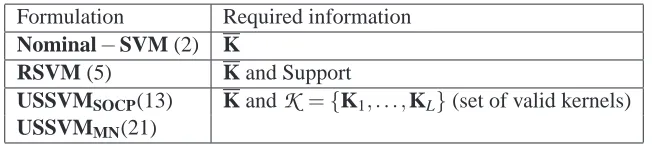
Formulation Required information

Nominal₋SVM (2) K

RSVM (5) K and Support

USSVMSOCP(13) K and

K

={K1, . . . ,KL}(set of valid kernels)

USSVMMN(21)

Table 1: Summary of Various formulations and associated Information required.

measure (RobustErr) which counts the fraction of data points in

D

for which there is atleast one error among R observations. More precisely

RobustErr(RE) =∑

ntst

t=11(∃s_|ys t6=yt)

ntst

(28)

is a more appropriate measure than (ME) to evaluate robustness.

In the following section, we report experimental results for the algorithms developed in this paper and benchmark them against the state of the art with respect to the above mentioned metrics.

7. Experimental Evaluation

This section presents experimental evaluation of the formulations, namely Nominal₋SVM, USSVMSOCP, USSVMMNand RSVM. The Nominal−SVM formulation is the usual SVM

for-mulation (2) with the nominal kernel. The minimax problem (12) when solved by the FSS procedure will be referred as USSVMMN. The solution of the SOCP (13) will be referred as USSVMSOCP.

Though as discussed before the setup of Bhadra et al. (2010) does not apply here but for sake of completeness we have also included a comparison with RSVM. A brief summary of the formula-tions is presented in Table 7.4

In particular it would be interesting to explore the following questions.

1. Comparison of USSVMSOCPand USSVMMNagainst the non-robust Nominal−SVM.

2. Convergence and scalability of USSVMMNalgorithm

The section is organized as follows. We begin by a brief description of data sets in Section 7.1. A comparative study of robustness is presented in Section 7.2. The first issue is discussed in Section 7.3. The experimental verification of the convergence rate of FSS procedure is discussed in Section 7.4. Next the scalability of USSVMMNover USSVMSOCPis discussed in Section 7.5.

7.1 Data Sets

We created synthetic data sets to test the generalization and robustness properties of the proposed formulations. Additionally we also have empirically tested them on protein structure data. We describe them below.

(17)

7.1.1 SYNTHETICDATASETS ANDKERNEL FUNCTIONS

It is important to evaluate the effect of robustness on wide variety of situations. To this end we use the following data generation mechanism suited for binary classification problems.

Choose d_∼U ni f(2,100), where U ni f(n1,n2)is the uniform distribution over all integers from n1to n2. For such a choice of d create a mixture distribution consisting of 4 Gaussian distributions, N(µ,Σ), with diagonal covariance matrix. The mean of each Gaussian distribution, µ_∈Rd_{, is} determined by independently choosing µj∼U ni f orm(−5,5) j=1, . . . ,d. Each diagonal entry of the diagonal matrixΣis independently drawn from U ni f orm(0,5). We assigned labels to the centers of each Gaussian distribution according to the sign(w⊤x) where w_∈Rd is a random vector with

kw_k=1. A data set of 2N points was generated as follows. First a set of N points corresponding to the positive class was generated by sampling N observations from the Gaussian mixture distribution consisting of positively labeled mixture components. The set of N points were generated from negatively labeled mixture components.

We study the problem of robust classification when the kernel values are not available but are governed by (10). Next we describe the construction of base kernels needed in (10). A linear kernel will be very effective for any data set D, created by the data generation process described. Given D=_{(xi,yi)|i=1, . . . ,N}we define K=x⊤i xj. Furthermore, L kernels were simulated as follows; Kl=K+ZlZl⊤, where Zi jl were generated using: a) Gaussian (0,1) b) Uniform [-1,1] c) centered Beta (0.5,0.5) distributions. After that, the generated values were multiplied by a random

li j ∼Uniform(0,0.05|Kij|). This leads to L valid positive semidefinite kernels for each of the

distribution, namely Gaussian, Uniform, or Beta.

We will denote by DG(S,N,L), the set of S data sets,{D1, . . . ,DS}. Each data set was created by the data-generation mechanism discussed earlier and has N examples per class with L kernels generated by the Gaussian distribution. Similarly DU(S,N,L) and DB(S,N,L)will correspond to

the Uniform and Beta distribution.

7.1.2 RESOLUTION-AWAREPROTEINSTRUCTURECLASSIFICATION

We have used a data set based on the SCOP (Murzin et al., 1995) 40% sequence non-redundant data set taken from Bhadra et al. (2010). The data set has 15 classes (SCOP superfamilies), having 10 structures each. The names of these superfamilies are reported in Appendix D. To study the effect of robustness we studied the classification problem on all possible pairs, which gave rise to 105 data sets in total. Each data set D can be thought of D=_{Pi,yi,ri|i=1, . . . ,n}where Pi is the nominal structure described in (3) with label yi. Incorporation of resolution information rileads to uncertainty sets U(Pi)(see (4)). Using the kernel function described in Bhattacharya et al. (2007) and assuming that the resultant uncertainty in kernel values obey (10) the kernel functions K,Klare computed by the procedure outlined in Section 4.3.

As described in the Section 3, the uncertainty set imposed by RSVM maynot always be appro-priate. However we still provide a comparison to the robust formulations described in this paper for the sake of completion. In the setting of the paper a set of kernel matrices

K

=_{K1,K2, . . . ,KL} are specified. The formulation RSVM needs support information, (see Table 7), which could be extracted as follows

K=1 L

L

∑

l=1

Kl ai j =min

(18)

The algorithms USSVMSOCP and USSVMMN and RSVM have been implemented in Matlab

with the help of Sedumi5 (Sturm, 1999). We have used libSVM6 as an SVM solver. All the ex-periments have been performed on a 64 bits Linux PC with 8 Intel Xeon 2.66 GHz processors and 16GB of RAM. The RSVM implementation uses a Quasi Newton procedure outlined in Bhadra et al. (2010). As it often gets stuck in a local minima we have used multiple starting points. All results on RSVM reported here corresponds to the results of the best starting point among 100 randomly selected starting points according to RSVM objective function.

7.2 Comparison of Robustness

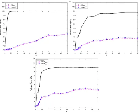
We begin by studying the effect of robustness on synthetic data. In the proposed model of uncer-tainty the parameterκplays a very important role. Whenκ=0, then there is no uncertainty and as it increases the uncertainty becomes more pronounced. The utility of robust formulations would become clear asκis increased. One would like to experimentally verify the fact that indeed this is the case. To this end we conducted the following experiment.

We created data sets DG(S,N,L),DU(S,N,L),DB(S,N,L) with S=10,N=250,L=200, as

described in Section 7.1. We have performed 5-fold cross-validation on all the 10 data set. Here we varyκ _{∈ {}0.1,0.2,0.3,0.5,1,1.5,2,2.5,3,3.5,4,5_}with R=100. In Figure 2, we have plotted the RobustErr (28) averaged over all 10 data sets for various distributions and choices ofκ. Though we get similar result for few different values of C here we have reported the results for the value of

C=100. Again DG will refer to the Gaussian distribution, DUrefers to the uniform case, and DB

refers to the Beta distribution.

The results of the experiment were as follows. It can be seen from Figure 2 that atκ=0, the RE for both USSVMSOCPand USSVMMNare exactly same as that of Nominal−SVM. It confirms the

fact that atκ=0, USSVMSOCP(USSVMMN)is equivalent to Nominal−SVM, as there is no

uncer-tainty. Figure 2 shows that, with the increase of uncertainty in the test examples, the RobustErr(28) for Nominal₋SVM increases substantially when compared to USSVMSOCP and USSVMMN on

all the 3 data sets. This shows that, non-robust classifiers, for example, SVM, are unable to handle uncertainty compared to the proposed robust classifiers. Also as expected both USSVMSOCPand

USSVMMNare equivalent and so on the test one they exhibit similar performance.

7.3 Comparison of Generalization Error

In this section we compare the error measures, RE (28) and ME (27).

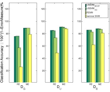
We again use the same data sets described in the previous subsection. For all the metrics, we have performed 5-fold cross-validation on all the 10 data sets corresponding to each distribution. The hyper-parameters (C and ε) for each classifier, were chosen using a grid search mechanism from the set C=_{0.1, 1, 5, 10, 50, 100, 200, 500_} andε=_{0.05+0.05step_|step=0, . . . ,9_}. For each metric, the cross-validation accuracy, 100(1₋ErrorMeasure)%, averaged over 10 data sets for various distributions, are reported in Figure 3. Note that DGrefers to the Gaussian case, DU

refers to Uniform case and DBrefers to the Beta case. The parameterκwas set to 1.

The results were as follows. All the formulations achieved an accuracy of 90% when NE was used as a error measure. From Figure 3 we see that both USSVMSOCP and USSVMMN beats

RSVM in terms of RE indicating that RSVM is not well suited for the uncertainty sets considered

5. Sedumi can be found athttp://sedumi.ie.lehigh.edu/.

(19)

Figure 2: Plot of RE for distributions (clockwise starting from top left )DG,DU,DBwith varyingκ.

Formulations compared are USSVMMN,USSVMSOCPand Nominal−SVM. The legend

SVM refers to Nominal₋SVM

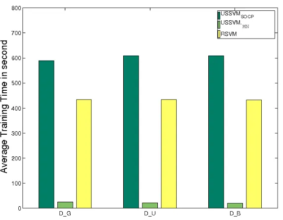
here. When we use ME, which is not as conservative as RE the gap narrows. This experiment demonstrates that in the presence of uncertainty the performance of extremely accurate classifiers suffer drastically but the proposed robust formulations fare much better in handling uncertainty. In addition, Figure 4 shows that the average training time of USSVMSOCP is same as that of RSVM

but USSVMMNis 10 times faster than both of them, even for these small scale data sets (200 training

datapoints per class).

7.4 Verification of Convergence of FSS Algorithm

In this section, we have experimentally verified that the proposed saddle point based algorithm has

O( 1

M2

s) convergence rate (see (20)). Recall that Ms is the actual number of steps, which one can

(20)

Figure 3: Cross-validation accuracy (%) obtained with USSVMSOCP, USSVMMN, RSVM and

Nominal₋SVM using RE (28)and ME (27). All values reported here are 100(1₋

Errormeasure)%

We report results on Data Set DU(1,N,5)where N∈ {50,500}, and C was chosen to be 1 for

N=50 and similarly for N=500 it was fixed to be 10.

Figure 5 shows the convergence rate of the Saddle Point based algorithm for USSVM formula-tion. The x-axis and the y-axis denote log10(Ms)and log10(εsad)respectively. All the points on the graph indicate the “end” of the sthstep and circled points indicate the “end” of the s_∗step. When

s>s∗, ideally the graph should be a straight-line with slope less than₋2 and one can observe the same in Figure 5. On the other hand, for s<s_∗rate of decrease inεsadis much slower than the case in s>s_∗.

7.5 Scalability of USSVMMN

In this section we study the relative performace of USSVMMNversus USSVMSOCPon large data

sets. We also verify the convergence criteria of proposed USSVMMN.

In the USSVMMNalgorithm the number of stages and the number of iterations inside one stage

(21)

dif-Figure 4: Average Training Time in Seconds obtained with USSVMSOCP, USSVMMN, and RSVM.

7 8 9 10 11 12 13 14 15 16

−14 −12 −10 −8 −6 −4 −2

log(M s)

log(

ε sad

)

C=1, N=50, S*=5 C=10, N=50, S*=6 C=1, N=500, S*=7 C=10, N=500, S*=7

Figure 5: Rate of convergence for Saddle point based algorithm

fer significantly. To this end we have compared the training times for USSVMSOCPand USSVMMN

(22)

Figure 6: Training time for USSVMSOCPUSSVMMNwith N= [500,1000,2000,3000,4000,5000]

and L= [10,50]

We have used synthetic data set generated similar to DU (please see Section 7.1) with number of data points in each class are_{250,500,1000,1500,2000,2500_}, where L=_{10,50_}. The values of R=100, C=10 andκ=1 were used.

Figure 6 shows training time (in sec) for varying N. One can observe that, with the increase of N, the training time for USSVMSOCP increases very steeply compared to the training time for

USSVMMN. As expected, training time for USSVM in general increases with the increase of

num-ber of uncertain kernels (L). As an example, to build a robust classifier with only 3000 data points,

USSVMSOCPneeds more than 5 hours while USSVMMNcompletes within 20 minutes. This

con-cludes that, to build a robust classifier with a medium scale of data (even more than 1000) the saddle point based algorithm is much more effective then a Quadratic Conic Program based formulation.

7.6 Discussion of Experimental Results

The results on the synthetic experiments show that USSVMSOCP,USSVMMNperforms better than

RSVM in terms of generalization as measured by various error measures. All the three formulations

are more robust than Nominal₋SVM. It is also demonstrated that USSVMMN is much more

scalable than USSVMSOCP. Even to build a robust classifier with 3000 data points, USSVMSOCP

needs more than 5 hours while USSVMMNcompletes within 20 minutes.

7.7 Resolution-aware Protein Structure Classification

(23)

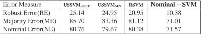
Error Measure USSVMSOCP USSVMMN RSVM Nominal−SVM

Robust Error(RE) 25.14 24.95 20.95 10.38

Majority Error(ME) 85.70 83.36 81.12 71.01

Nominal Error(NE) 80.76 79.67 80.38 71.57

Table 2: Comparison of USSVMSOCP, USSVMMN RSVM and Nominal−SVM using accuracy

measures, 100(1₋ErrorMeasure)%, where Error measures are defined in Section 6.2. Table shows average accuracy for all 105 one-vs-one classification problems

The data set is described in Section 7.1. The experimental methodology follows “one-vs-one” classification setting with all 15 classes of protein structures. Leave-One-Out (LOO) cross valida-tion using SVM, RSVM and USSVM was performed on all 105 of such classificavalida-tion problem. In all cases we report accuracy, computed as 100(1₋ErrorMeasure)%.

Let

D

=_{(Pi,ri,yi)}be a protein structure data sets where Piis the set of coordinates of ith pro-tein structure obtained from Astral7database, where riis the corresponding resolution information obtained from the PDB, and yi is the class label. Using resolution information, we generated a set of perturbed structures Qi={Pi1, . . . ,PiL}for each Pi as follows. For each atom pia of Pigenerated

structure P_is with coordinates of atoms as pl_i_a =pia+u and u∼U(−

ri

2 ,

ri

2). One can create a set

of uncertain kernels, where K(p,p′)is a kernel function computed between two protein structures

p_∈Qi and p′∈Qj. For our experiments, we have generated a set of kernels consisting of L=50 base kernels. Denoting the kernel matrices by{K1, . . . ,KL}the uncertainty set is defined as

E

(1)

(see (11)) with K= 1_L∑L_l₌₁Kl andκ=1. Given the base kernels the prediction is implemented,

as reported in Section 6, with R=100 andκ=1. For the purpose of our comparison, we have used weighted pair-wise distance substructure kernel (Bhattacharya et al., 2007). These kernels are purely based on protein structure (specially position of cα). Please refer to Appendix C for details. For RSVM, we compute the following,

Ki j=Ki j,ai j= min p∈Qi,p′∈Qj

K(p,p′),bi j= max p∈Qi,p′∈Qj

K(p,p′).

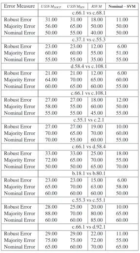
7.7.1 RESULTS ONPROTEINSTRUCTURECLASSIFICATION

Table 2 and Table 3 report results for RSVM, USSVMMNand Nominal−SVM (SVM with kernels

based on nominal protein structure reported in PDB files) using both standard and robust error measures defined in section 6.2 in the Leave-One-Out (LOO) procedure. Hyper-parameters (C and/orε) for RSVM and C for USSVMMN and Nominal−SVM were tuned separately using the

grid search mechanism. As this is a 15 class classification problem and we followed a “one-vs-one” setting, we have reported average accuracy of all 105 classifiers (Table 2). We have also provided a list of a few individual classes (Table 3) where U SSV M performed significantly better than RSVM. The results are presented in the form of a histogram of performance differences (%) of U SSV M against RSV M and SV M obtained by using RE (28) in Figure 7.

It is clear that RSVM, and USSVM perform significantly better than their non-robust coun-terparts, both in terms of Accuracy (measured by MajorityErr) and Robustness (measured by Ro-bustErr). This result indicates that, the use of resolution information improves the overall

(24)

−2 0 2 4 6 8 10 12 14 0

5 10 15 20 25 30

100*(1−RE) of USSVM

SOCP − 100(1−RE) of RSVM

Number of classifiers

8 10 12 14 16 18 20 22

0 5 10 15 20 25 30 35

100*(1−RE) of USSVM

SOCP − 100*(1−RE) of SVM

Number of classifiers

Figure 7: Histogram of performance differences (%) between USSVMSOCP and RSVM is shown

in the top figure. The bottom figure corresponds USSVMSOCP and SVM

tion accuracy. In fact, USSVM even beats RSVM in terms of robustness. Note that, for more than 50% classification problem accuracy of USSVMSOCP is more than 5% of that of RSVM in terms

of Robustness. For few classes difference in accuracy was more than 10% (see Table 3). More-over, this performance difference increases while comparing USSVM against Nominal₋SVM.

For more than 60% classification problem accuracy of USSVMSOCPis more than 15% of that of

Nominal₋SVM in terms of robustness and notably for almost all the cases the margin was more

than 10% in term of RobustErr.

8. Conclusion

(25)

Error Measure U SSV MSOCP U SSV MMN RSV M Nominal−SVM

c.66.1 vs c.68.1

Robust Error 31.00 31.00 18.00 11.00

Majority Error 56.00 65.00 50.00 50.00

Nominal Error 50.00 55.00 40.00 50.00

c.37.1 vs c.55.3

Robust Error 23.00 23.00 12.00 6.00