Word Sequence Kernels

Word-Sequence Kernels

Nicola Cancedda [email protected]

Eric Gaussier [email protected]

Cyril Goutte [email protected]

Jean-Michel Renders [email protected]

Xerox Research Centre Europe 6, chemin de Maupertuis 38240 Meylan, France

Editors: Jaz Kandola, Thomas Hofmann, Tomaso Poggio and John Shawe-Taylor

Abstract

We address the problem of categorising documents using kernel-based methods such as Support Vector Ma-chines. Since the work of Joachims (1998), there is ample experimental evidence that SVM using the standard word frequencies as features yield state-of-the-art performance on a number of benchmark problems. Re-cently, Lodhi et al. (2002) proposed the use of string kernels, a novel way of computing document similarity based of matching non-consecutive subsequences of characters. In this article, we propose the use of this technique with sequences of words rather than characters. This approach has several advantages, in particular it is more efficient computationally and it ties in closely with standard linguistic pre-processing techniques. We present some extensions to sequence kernels dealing with symbol-dependent and match-dependent decay factors, and present empirical evaluations of these extensions on the Reuters-21578 datasets.

Keywords: Kernel machines, text categorisation, linguistic processing, string kernels, sequence kernels

1. Introduction

The application of machine learning techniques to classification of documents is a rich and challenging re-search area with many related tasks, such as routing, filtering or cross-lingual information retrieval. Since Joachims (1998) and other researchers like Yang and Liu (1999) have shown that Support Vector Machines (SVM) perform favourably compared to competing techniques for document categorisation, kernel machines have been a popular choice for document processing. In most reported works, however, documents were rep-resented using the standard vector space, aka bag-of-word model (Salton and McGill, 1983)—that is, more or less, word frequencies with various added normalisations—in conjunction with general purpose kernels (linear, polynomial, RBF, etc.).

Recently, Watkins (1999) and Lodhi et al. (2001, 2002) proposed the use of string kernels, one of the first significant departures from the vector space model. In string kernels, the features are not word frequencies or an implicit expansion thereof, but the extent to which all possible ordered subsequences of characters are represented in the document. In addition, Lodhi et al. (2001) proposed a recursive dynamic programming formulation allowing the practical computation of the similarity between two sequences of arbitrary symbols as the dot-product in the implicit feature space of all ordered, non-consecutive subsequences of symbols. Al-though it allows to perform the kernel calculation without performing an explicit feature space expansion, this formulation is extremely computationally demanding and is not applicable (with current processing power) to large document collections without approximation (Lodhi et al., 2002).

corpus becomes feasible without approximation. In addition, matching sequences of words allows to work with symbols that are expected to be more linguistically meaningful. This leads to extensions of the word sequence kernels that implement a kind of inverse document frequency (IDF) weighting by allowing symbol-varying decay factors. Words may also be equivalent in some context, and we show how to implement soft word matching in conjunction with the word-sequence kernel. This allows the use of this kernel in a multi-lingual context, an application that was not possible with the string kernel formulation.

In Section 2 we offer a brief self-contained introduction to kernel methods, after which we will proceed with the presentation of sequence kernels (Section 2.2). Section 3 formulates and verifies a hypothesis that helps explain why string kernels perform well, even though they are based on processing entities (characters) which are essentially meaningless from a linguistic point of view. Section 4 presents our extension of se-quence kernels to word-sese-quences, which we test empirically in Section 4.2. Finally, we present in Section 5 some extensions of word-sequence kernels to soft-matching and cross-lingual document similarity.

2. Kernel Methods

Kernel methods are a research field in rapid expansion. Based on theoretical work on statistical learning theory (Vapnik, 1995) and reproducing kernel Hilbert spaces (Wahba, 1990), kernel machines were first popular as SVM (Boser et al., 1992, Cortes and Vapnik, 1995). In this section we will briefly introduce kernel-based classifiers and sequence kernels. For additional information, the reader may refer to general introductions such as Cristianini and Shawe-Taylor (2000), Sch¨olkopf and Smola (2002) or Herbrich (2002).

2.1 Kernel Classifiers

A binary classifier is a function from some input space

X

into the set of binary labels{−1,+1}. A supervised learning algorithm is a function that assigns, to each labeled training set S∈(

X

× {−1,+1})l, a binary classifier h :

X

→ {−1,+1}. For computational reasons and in order to limit overfitting, learning algorithms typically consider only a subset of all classifiers,

H

⊂ {h|h :

X

→ {−1,+1}}, the hypothesis space. In the common case in which

_X

is a vector space, one of the simplest binary classifiers is given by the linear discriminant:

h(x) =sign(hw,xi+b)

whereh·,·idenotes the standard dot-product. Learning the linear classifier amounts to finding values of w and b which maximise some measure of performance. Learning algorithms for linear classifiers include e.g. Fisher’s linear discriminant, the Perceptron and SVM. All linear classifiers will naturally fail when the boundary between the two classes is not linear. However, it is possible to leverage their conceptual simplicity by projecting the data from

X

into a different feature space

F

in which we hope to achieve linear separation between the two classes. Denoting the projection into feature space byφ:

X

→

F

, the generalised linear classifier becomes:

h(x) =sign(hw,φ(x)i+b) (1)

The separating hyperplane defined by w and b is now in the feature space

F

, and the corresponding classifier in the input space

X

will generally be non-linear. Note also that in this setting,

X

need not even be a vector space as long as

F

is. This is a crucial observation for the rest of this article, as we will be dealing with the case in which

X

is the associative monoid of the sequences over a fixed alphabet, which is not a vector space.

In the case of SVM, the optimal weightsw can be expressed as a linear combination of the data:b

b w=

l

∑

i=1

yiαiφ(xi) (2)

whereαi∈Ris the weight of the i-th training example with input xi∈

X

and label yi∈ {−1,+1}.

Accord-ingly, by combining (1) and (2), the SVM classifier can be written in its dual form:

h(x) =sign

l

∑

i=1

yiαihφ(x),φ(xi)i+b

!

Notice that the projectionφonly appears in the context of a dot product in (3). In addition, the optimal weights(αi)are the solution of a high dimensional quadratic programming problem which can be expressed

in terms of dot products between projected training datahφ(xi),φ(xj)i. Rather than use the explicit mapping

φ, we can thus use a kernel function K :

X

×

X

→Rsuch that K(x,y) =hφ(x),φ(y)i. As long as K(x,y)can be calculated efficiently, there is actually no need to explicitly map the data into feature space usingφ—this is the kernel trick. It is especially useful when the computational cost of calculatingφ(x)is overwhelming (e.g., when

F

is high dimensional) while there is a simple expression for K(x,y). In fact, Mercer’s theorem (see, e.g. Cristianini and Shawe-Taylor, 2000, Section 3.3.1) states that any positive semi-definite symmetric function of two arguments corresponds to some mappingφin some space

_F

and is thus a valid kernel. This means that in principle a kernel can be used even if the nature of the corresponding mappingφis not known. This article addresses the application of kernel methods to the well known problem of document cate-gorisation. So far, most of the kernel-based work in this area used a standard bag-of-words representation, with word frequencies as features, ie

_X

=Rn_{. Although these vector representations have proved largely}

suc-cessful, we will here investigate the use of representations which are intuitively closer to the intrinsic nature of documents, namely sequences of symbols. This representation does not form a vector space, but the use of appropriate kernels will allow us to leverage the discriminative power of kernel-based algorithms. As we will see, the kernels we are going to consider will also allow us to test basic factors (e.g., order or locality of multi-word terms) in the context of document categorisation.

2.2 Sequence Kernels

The assumption behind the popular bag-of-words representation is that the relative position of tokens has little importance in most Information Retrieval (IR) tasks. Documents are just represented by word frequen-cies (and possibly additional weighting and normalisation), and the loss of the information regarding the word positions is more than compensated for by the use of powerful algorithms working in vector space. Although some methods inject positional information using phrases or multi-word units (Perez-Carballo and Strzalkowski, 2000) or local co-occurrence statistics (Wong et al., 1985), the underlying techniques are based on a vector space representation.

String kernels (or sequence kernels) are one of the first significant departures from the vector-space rep-resentation in this domain. String kernels (Haussler, 1999, Watkins, 1999, Lodhi et al., 2001, 2002) are similarity measures between documents seen as sequences of symbols (e.g., possible characters) over an al-phabet. In general, similarity is assessed by the number of (possibly non-contiguous) matching subsequences shared by two sequences. Non contiguous occurrences are penalized according to the number of gaps they contain.

Formaly, let Σbe a finite alphabet, and s=s1s2...s|s| a sequence overΣ(i.e. si∈Σ,1≤i≤ |s|). Let

i= [i1,i2,...,in], with 1≤i1<i2< ... <in≤ |s|, be a subset of the indices in s: we will indicate as s[i]∈Σn

the subsequence si1si2...sin. Note that s[i] does not necessarily form a contiguous subsequence of s. For

example, if s is the sequence CART and i= [2,4], then s[i]is AT . Let us write l(i)the length spanned by s[i] in s, that is: l(i) =in−i1+1. The sequence kernel of two strings s and t overΣis defined as:

Kn(s,t) =

∑

u∈Σn_i:s

∑

_[i]=uj:t

∑

_[j]=u

λl(i)+l(j) ₍₄₎

whereλ∈]0; 1]is a decay factor used to penalise non-contiguous subsequences and the first sum refers to all possible subsequences of length n. Equation 4 defines a valid kernel as it amounts to performing an inner product in a feature space with one feature per ordered subsequence u∈Σnwith value:

φu(s) =

∑

i:s[i]=u

λl(i) ₍₅₎

A direct computation of all the terms under the nested sum in (4) becomes impractical even for small values of n. In addition, in the spirit of the kernel trick discussed in Section 2, we wish to calculate Kn(s,t)

directly rather than perform an explicit expansion in feature space. This can be done using a recursive formulation proposed by Lodhi et al. (2001), which leads to a more efficient dynamic-programming-based implementation. The derivation of this efficient recursive formulation is given in appendix A, together with an illustrative example. It results in the following equations:

K₀0(s,t) = 1, for all s,t,

for all i=1,...,n−1:

K_i00(s,t) = 0, if min(|s|,|t|)<i (6)

K_i0(s,t) = 0, if min(|s|,|t|)<i (7)

K_i00(sx,ty) = λK_i00(sx,t) iff y6=x (8)

K_i00(sx,tx) = λK_i00(sx,t) +λ2K_i0₋₁(s,t) otherwise (9)

K_i0(sx,t) = λK_i0(s,t) +K_i00(sx,t) (10)

and finally:

Kn(s,t) = 0, if min(|s|,|t|)<n (11)

Kn(sx,t) = Kn(s,t) +

∑

j:tj=x

λ2_K0

n−1(s,t[1 : j−1]) (12)

The time required to compute the kernel according to this formulation is O(n|s||t|). In some situations, it may be convenient to perform a linear combination of sequence kernels with different values of n. Using the recursive formulation, it turns out that computing all kernel values for subsequences of lengths up to n is not significantly more costly than computing the kernel for n only. In order to keep the kernel values comparable for different values of n and to be independent from the length of the strings , it may be advisable to consider the normalised version:

ˆ

K(s,t) =p K(s,t)

K(s,s)K(t,t) (13)

This is a generalisation of the “cosine normalisation” which is widespread in IR and corresponds to the mapping ˆφ(s) =_kφφ₍(_ss₎)_k

2 (wherek.k2is the 2-norm).

3. The Noisy-Stemming Hypothesis

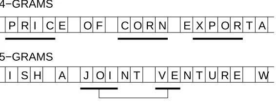
Text categorisation using string kernels operating at the character level has been shown to yield performance comparable to kernels based on the traditional bag-of-words representation (Lodhi et al., 2001, 2002). This result is somewhat surprising, considering string kernels use only low-level information. A possible expla-nation of the effectiveness of the string kernel, supported by the observation that performance improves with n, is that subsequences most relevant to the categorisation may correspond to noisy versions of word stems, thus implicitly implementing some form of morphological normalisation. Furthermore, as gaps within the sequence are allowed —although penalized— string kernels could also pick up stems of consecutive words, as illustrated in Figure 1. This is known to help in IR applications (Salton and McGill, 1983).

In order to test this noisy stemming hypothesis, the following experiment was conducted. An SVM using a string kernel was trained on a small subset of the Reuters-21578 corpus,1using the labels for theacqtopic. A sample of features—subsequences of a fixed length n—was randomly chosen. In order to avoid a vast majority of irrelevant low-weight features, we restricted ourselves to possibly non-contiguous subsequences appearing in the Support Vectors. For each sampled feature u, its impact on the categorisation decision was compared to a measure of stemnessσu. The impact on the categorisation decision is measured by the absolute

I E O F

C O N

E

P R

C

R

X P O R

T

A

H A J O I N T

V

E

N

I S

T U R E

W

4−GRAMS

5−GRAMS

Figure 1: The noisy-stemming hypothesis. N-grams may be able to pick parts of words/stems (top, with n=4) or even pick parts of stems of consecutive words (bottom, n=5).

weight wuin the linear decision:

wu=

∑

_j αjyjφu(xj)

In order to assess the stemness of a feature, ie the extent to which a feature approximates a word stem, a simplifying assumption was made by considering that stems are the initial characters in a word. Moreover, in order to verify that a feature may span two consecutive stems, a measure of stemness was devised so as to consider pairs of consecutive tokens. Let t={t1,...,tm}, with 1=t1<t2< ... <tm<tm+1=|s|+1, be a

tokenisation of the string s (the tokenisation is the segmentation process that provides the indices of the first symbol of each token). Let m(k,u)be the set of all matches for the subsequence u in the pair of consecutive tokens starting in tk−1and tkrespectively, with 2≤k≤m:

m(k,u) = i0,i00|u=s[i0]s[i00],tk−1≤i01≤i0|i0|<tk≤i001≤i00|i00|<tk+1

In a matching pair where i0=/0, the constraint tk−1≤i0|i0|<tkis considered automatically satisfied. In

addition, i00is forced to be different from /0, in order to avoid double counting of single word matches, and an empty symbol is added at the beginning of the string to allow one-word matching on the first token. The stemness of a subsequence u with respect to s is then defined as:

σu(s) =avgk:m(k,u)6=/0

λmin_m(k,u)

i0_|i0|−tk−1−|i0|+i00_|i00|−tk−|i00|

In other words, for each pair of consecutive tokens containing a match for u, a pair of indices(i0,i00)is selected such that s[i0]matches into the first token, s[i00]matches in the second and each component is found as compact and close to the start of the corresponding token as possible. The stemness of u with respect to the whole training corpus is then defined as the (micro-)average of the stemness in all documents in the corpus. This experiment was performed with a sample of 15000 features of length n=3, and a sample of 9000 features of n=5, withλ=0.5 in both cases. Under the noisy-stemming hypothesis, we expect relatively few features with high weight and low stemness. The outcome of our experiment, presented in Table 1, seems to confirm this. For n=3, among features with high weight (>0.15) about 92% have high stemness, whereas among features with low weight the fraction of features with high stemness is of 73%. Similar results were found for n=5 (90% and 46% respectively).

For each non-empty set of matches m(k,u)6=/0, stemness is calculated by first finding the most compact match(i0_c,i00_c) =argmin₍i0,i00)∈m(k,u) i0|i0|−tk−1− |i0|+i00|i00|−tk− |i00|

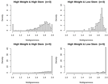
. It is interesting to check how often this “minimal” subsequence matches on two tokens, as opposed to single-token match. For that purpose, we define g(k,u) =1 if the most compact match is on one token (i.e. i_c0 = /0) and g(k,u) =2 otherwise. The multigramness of a subsequence u on sequence s is then:

n=3 wu

σu low high

low 3622 125

high 9877 1376

n=5 wu

σu low high

low 4413 86

high 3686 815

Table 1: Contingency tables for weight against stemness. Left (n=3, ie trigrams): Weights are split at 0.15 to separate the lowest 90% and highest 10% values, whereas stemness is split at 0.064 to separate the 25% lowest and 75% highest values. Right (n=5): Weights are split at 0.0066 to separate the lowest 90% and highest 10% values, whereas stemness is split at 0.029 to separate the 50% lowest and 50% highest values. Theχ2_{values for the tables are 247 (left) and 655 (right), which suggests} a highly significant departure from independence in both cases (1 d.o.f.).

High Weight & High Stem (n=3)

Multigramness

Density

1.0 1.2 1.4 1.6 1.8 2.0

02468

1

0

High Weight & Low Stem (n=3)

Multigramness

Density

1.0 1.2 1.4 1.6 1.8 2.0

02468

1

0

High Weight & High Stem (n=5)

Multigramness

Density

1.0 1.2 1.4 1.6 1.8 2.0

0

1

02

03

04

0

High Weight & Low Stem (n=5)

Multigramness

Density

1.0 1.2 1.4 1.6 1.8 2.0

0

1

02

03

04

0

Figure 2: Density of “Multigramness” for high weight features, n=3 and n=5.

Using the same feature samples as above, we estimate the distribution of γu(s)for features with high

weights (the most interesting features). Figure 2 shows that the mass of each distribution is close to 2, indicating that matching occurs more often on more than one word. This effect is even clearer for larger n: high weight features of length n=5 are concentrated nearγu=2. This is reasonable considering longer

subsequences are harder to match on a single word. On the other hand, a significant amount of high weight, high stemness features of length n=3 are clearly single stem features. In addition, features with high weight but low stemness have a tendency to spread on two stems (right column vs. left column in Figure 2).

4. Word-Sequence Kernels

The seeming validity of the noisy-stemming hypothesis suggests that sequence kernels operating at the word (possibly word-stem) level might prove more effective than those operating at the character level. In this section, we describe the impact of applying sequence kernels at the word level, and extend the original kernel formulation so as to take into account additional information.

4.1 Theory

The direct application of the sequence kernel defined above on an alphabet of individual words raises some significant issues. First, the feature space on which documents are implicitly mapped has one dimension for each of the|Σ|n ordered n-tuples of symbols in the alphabet: going from characters to words, the order of magnitude of|Σ|increases from the hundreds to the tens of thousands, and the number of dimensions of the feature space increases accordingly. However, the average length in symbols of documents decreases by an order of magnitude. As the algorithm used for computing sequence kernels depends on sequence length and not on alphabet size, this yields a significant improvement in computing efficiency: word-sequence kernels can be computed on datasets for which string kernels have to be approximated.

Nevertheless, the combination of the two effects (increase in alphabet size, decrease in document average length) causes documents to have extremely sparse implicit representations in the feature space. This in turn means that the kernel-based similarity between any pair of distinct documents will tend to be small with respect to the “self-similarity” of documents, especially for larger values of n. In other words, the Gram matrix tends to be nearly diagonal, meaning that all examples are nearly orthogonal. In order to overcome this problem, it is convenient to replace the fixed-length sequence kernel with a combination of sequence kernels with subsequence lengths up to a fixed n. A straightforward formulation is the following 1-parameter linear combination:

¯

Kn(x,y) = n

∑

i=1

µ1−iKˆi(x,y) (14)

Considering the dynamic programming technique used for the implementation, computing the sequence ker-nel for subsequences of length up to n requires only a marginal increase in time compared to the computation for subsequences of length n only. Notice that kernel values for different subsequence lengths are normalised independently before being combined. In this way it is possible to control the relative weight given to differ-ent subsequence lengths directly by means of the parameter µ. The µ parameter, or possibly the parameters of a general linear combination of sequence kernels of different orders, can be optimized by cross-validation, or alternatively by kernel alignment (Cristianini et al., 2001).

In its original form, the sequence kernel relies on mere occurrence counts, or term frequencies, and lacks feature weighting schemes which have been deemed important by the IR community. We want to present now two extensions to the standard sequence kernel. The first uses different values ofλto assign different weights to gaps, and allows the use of well-established weighting schemes, such as the inverse document frequency (IDF). It can also be used to discriminate symbols according to, say, their part-of-speech. The second extension consists in adopting different decay factors for gaps and for symbol matches, and generalises over the previous extension in the sense that informative symbols are treated differently depending on whether they are used in matches or gaps.

4.1.1 SYMBOL-DEPENDENTDECAY FACTORS

introduce a distinctλxfor each x∈Σ. This induces the following new embedding:

φu(s) =

∑

i:s[i]=ui1<

∏

j<in

λsj

The value of the feature u=gas injection in the sequence s=gas assist plastic injection is then: φu(s) =λgasλassistλplasticλinjection

The corresponding weighted sequence kernel Kwis thus defined as follows:

K_wn(s,t) =

∑

u∈Σn

φu(s)φu(t) =

∑

u∈Σn_i:u

∑

_=s[i]j:u

∑

_=t[j]i

∏

1≤k≤in

∏

j1≤l≤jn

λskλtl.

A recursive formulation analogous to the one for the original sequence kernel can be derived. We can define functions Kw0and Kw00to store intermediate results (see Appendix A):

Kw0i(s,t) =

∑

u∈Σi_i:u

∑

_=s[i]j:u

∑

_=t[j]i1≤

∏

_k≤|s|j1≤

∏

_j≤|t|

λskλtj, for i=1,...,n−1

Kw00i(sx,t) =

∑

j:tj=x

Kw0i−1(s,t[1 : j−1])λx

∏

j≤l≤|t|

λtl,

and use the general recursion equations given in Section 2.2, with the following modifications: replaceλby λyin Equation 8, and byλxin Equations 9, 10 and 12.

Using different values ofλ is one way of incorporating prior knowledge into the sequence kernel. In the case of word-sequence kernels, for instance, symbols (i.e. words) could be grouped according to their part-of-speech. By doing so it is possible, for instance, to penalize more heavily occurrences with extraneous nouns, such as gas assist plastic injection, than occurrences with extraneous adverbs, as gas only injection. The rationale behind this is that the latter sequence is semantically closer to gas injection than the former (indeed, the plastic, and not the gas, is the main substance being injected in the former sequence).

This same extension can be useful—in the case of word-sequence kernels—in order to integrate informa-tion on the inverse document frequency of terms. A broadly used formula for taking IDF into account in term weighting schemes is:

idfc=log

N Nc

(15)

where N is the number of documents in the collection and Ncis the number of documents containing term c.

This formula yields a value between 0 and log(N)(only terms occurring in the collection are given non-zero weight), and need be normalised to be used as a decay factor:

λc=

log(_NN

c)

log(N) (16)

However, one can notice that there is a tension between the different types of information which can be integrated. On the one hand, words pertaining to certain parts-of-speech tend to be non discriminative when inserted in sequences (as only in the example above), and should thus be assigned highλ’s. But at the same time, the very same words tend to appear in many different documents, thus leading to lowλ’s when an IDF based weighting scheme is used. The second extension we propose solves this problem.

4.1.2 INDEPENDENTDECAYFACTORS FORGAPS ANDMATCHES

strongly penalized (i.e.:λcsmall), but highly relevant matching symbols to be rewarded (i.e.:λclarge). This

requirement cannot be met with the previous formulation.

One way to obtain the desired behaviour is to introduce two separate sets of decay factors for gaps and for matches. The u coordinate of the feature vector for the sequence s is now defined by

ˆ

φu(s) =

∑

i:u=s[i]1≤

∏

j≤|u|

λm,uj

∏

i1<k<i|u|,k6∈i

λg,sk (17)

whereλg,xis the discount factor for the symbol x when it occurs as a gap, andλm,xis the discount factor for

the same symbol when it occurs as a matching symbol. With this definition one could, for instance, discount gaps according to part-of-speech and weight matching symbols according to inverse document frequency information. The value of the feature u=gas injection in the sequence s=gas only injection would thus be:

φu(s) =λm,gasλg,onlyλm,injection

and we now have a way to consider only as unimportant when it appears in a gap (λg,only close to 1), and

uninformative when it appears in a match (λm,onlyclose to 0.). We now define the weighted sequence kernel

Kdwof two sequences s and t as

K_dwn(s,t) =

∑

u∈Σn

ˆ

φu(s)φˆu(t) (18)

=

∑

u∈Σn_i:u

∑

_=s[i]j:u

∑

_=t[j]1≤

∏

_j≤|u|

λ2

m,uj

∏

i1<k<i|u|,k6∈i

λg,sk

∏

j1<l<j|u|,l6∈j

λg,tl

As for the evaluation of Kdw, we define Kdw0and Kdw00as:

Kdw0i(s,t) =

∑

u∈Σi_i:u

∑

_=s[i]j:u

∑

_=t[j]

i

∏

k=1

λ2

m,ui

∏

i1<l≤|s|,l6∈i

λg,sl

∏

j1<r≤|t|,r6∈j

λg,tr,

Kdw00i(sx,t) =

∑

j:tj=x

Kdw0i−1(s,t[1 : j−1])λ2m,x

|t|

∏

l=j+1

λg,tl, for i=1,...,n−1.

and use the general recursion equations given in Section 2.2, with the following modifications: replaceλby λg,yin Equation 8, replace Equation 9 with

Kdw00i(sx,tx) =λg,xKdw00i(sx,t) +λ2m,xKdw0i−1(s,t)

replaceλbyλg,xin Equation 10 and replaceλbyλm,xin Equation 12.

This formulation shows that considering separate sets of decay factors for matching symbols and for gaps does not impact the computational complexity of the kernel. In the remainder of the paper, we will refer to the extension corresponding to Equation 17, as the word-sequence kernels with symbol-dependent matching scores and decay factors.

4.2 Experiments

Word-sequence kernels generalise over previously introduced methods in several respects:

• For n=1, individual terms are matched. This amounts to performing the usual cosine measure between document vectors (once the kernel is normalised). If symbol-dependent matching scores and decay factors are adopted, IDF based weighting schemes can be enforced;

• Forλg=0, only contiguous sequences are matched, and the sequence kernel amounts to computing

a similarity between documents based on the number of n-grams (more precisely on the number of 1-gram, 2-grams, ... up to n-grams) they share;

• With varyingλg, the constraint on the contiguity of sequences can be relaxed, which suggests a way to

test whether locality of multi-word terms (i.e. the fact that words of a sequence appear relatively close to each other) is an important factor or not.

As we see, word-sequence kernels define a paradigm from which it is possible to test the importance of different, basic factors for the document categorisation task. Assessing the validity of these factors, as well as the performance of word-sequence kernels, is the goal of the experiments we designed. More precisely, we want to answer the following questions:

1. Does the knowledge of the order in which the matched terms of a sequence occur improve the quality of the similarity measure? In other words, does a word-sequence kernel withλ=1 perform better than the corresponding polynomial kernel?

2. Does the knowledge of the distance at which the matched terms of a sequence occur improve the quality of the similarity measure? That is, does a word-sequence kernel withλ<1 perform better than the same one withλ=1? Similarly, how does the version withλg=0 (i.e. the n-gram version) compare

to a more flexible word-sequence kernel in which the contiguity constraint is partially removed?

3. What relative importance should be given to individual words and to combination of words as indexing features? In other words, how does the parameter µ affect performance?

4. Do results improve if combination of more and more words are considered? How is performance affected by the value of n?

5. Is it actually useful to use symbol-dependent matching scores and decay factors? Related to this point is the questioning: is the word-sequence kernel sensitive to IDF based weighting schemes?

6. Finally, how does the word-sequence kernel compare to other kernels for text categorisation?

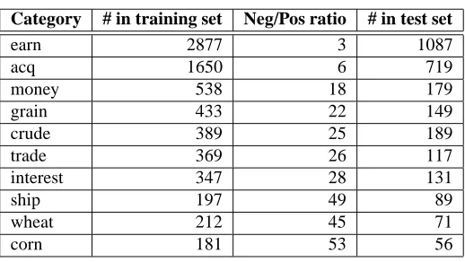
In order to answer these questions we performed a series of experiments using a standard benchmark for text categorisation systems: the Reuters-21578 corpus. We adopted the so-called “ModApte split”, which leads to a training set of 9603 documents and a test set of 3299. Although computationally far more tractable than sequence kernels operating at the character level (note that the standard string kernels cannot be directly computed on this collection, and need be approximated, as mentioned in Lodhi et al. (2002)), word-sequence kernels are still somewhat resource-demanding.2 We thus decided to limit our attention to the ten most frequent categories. Some characteristics of the composition of the training and test set relative to these categories are summarised in Table 2.

Documents were preprocessed by performing lemmatisation and resolving ambiguities by means of a part-of-speech tagger. Xerox tools were used to this effect. Lemmatisation maps different morphological variants of a same word (e.g. singular/plural forms of nouns, present/past tenses of verbs) onto the same feature (the lexeme). The underlying assumption is that the “inflected” form does not bring extra useful infor-mation compared to the “normalised” form. Notice however that many words are ambiguous (e.g. “saw”) and determining the correct lemma (in our example, “saw” as noun, “saw” as verb or “see” as verb) for each is non-trivial. This is the reason why a part-of-speech (POS) tagger is used: the tagger model is able to choose (i.e. disambiguate) one POS category according to the word’s context. After preprocessing, the number of features is about 53,000 and the average document length is 141 (when stopwords are removed, the average length drops to 77).

Category # in training set Neg/Pos ratio # in test set

earn 2877 3 1087

acq 1650 6 719

money 538 18 179

grain 433 22 149

crude 389 25 189

trade 369 26 117

interest 347 28 131

ship 197 49 89

wheat 212 45 71

corn 181 53 56

Table 2: Number of positive examples in the ten most frequent categories of the Reuters-21578 corpus (ModApte split).

Experiments were conducted using the SVMlight(Joachims, 1999) package,3version 3.50, appropriately adapted for using sequence kernels.4Training sets for all categories are all more or less unbalanced in favour of negative examples. This is a well known problem with the SVM algorithms, which implicitly tends to maximise accuracy, thus leading to learning overly conservative classifiers. SVMlight provides a parameter, however, to weight the relative importance of positive and negative examples in the training set. As a heuristic rule, all experiments were run with this parameter set at the integer value closest to the ratio between negative and positive examples in the training set. While there is no evidence that this setting optimises any of the measures usually adopted in IR, this seemed a reasonable choice to at least reduce the impact of the lack of balance in the training set.

PERFORMANCE EVALUATION

In the following experimental results, we use standard IR performance measures. From the test categorisation results, we calculate the true positives TP (number of documents the model correctly identifies as positives), the false positives FP (number of documents the model falsely identifies as positives) and the false negatives FN (number of documents the model fails to identify as positives). From these counts, we calculate the following performance measures:

Precision: the ratio of true positives among all retrieved documents, p=_{T P}T P_+FP.

Recall: the ratio of true positives over all positives, r=_{T P}T P_+FN.

F-score: the harmonic mean of precision and recall, F1=_p2pr_+r.

Note that these measures depend on the threshold that is applied to the decision function in order to decide whether a document is relevant. In order to provide a threshold-independent measure, we also compute the break-even point, which is the performance obtained at the threshold for which p=r. By definition, at the break-even point, precision, recall and F-score are equal.

In the remainder of this section, most experimental results are centered around a “reference” setting of µ=0.5, in which the weight of terms of size n is double that of terms of order n−1. We will see that this setting does not in general yield optimal performance. Note, however, that we study the impact of factors, such as order, locality or multi-term length, which control the way in which single-word terms interact with multi-word terms. In that context, using such a small value of µ gives more importance to longer terms, making this impact more visible.

3. Available at http://svmlight.joachims.org/

micro-average macro-average

p r F1 BP p r F1 BP

Stopwords not removed 91.98 87.62 89.75 90.21 85.20 74.30 78.92 80.86

Stopwords removed 93.01 88.09 90.52 91.46 85.37 76.71 80.64 83.09

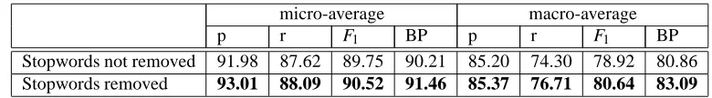
Table 3: The effect of removing stopwords on Precision (p), Recall (r), F1score and Break-even Point (BP). These results are obtained with n=2,λ=0.5 and µ=0.5.

The performance measures presented above are calculated for each category. In order to present a synthetic measure of performance over all categories, we present the micro-averaged and macro-averaged performance. Macro-averaging consists in simply averaging the results obtained on each category, while micro-averaging averages over individual decisions made on each document for each category. In effect, micro-averaging is dominated by the performance of “large” categories, while macro-averaging gives equal influence to all categories. In all our experiments, both methods give consistent results. However, as micro-averaging is dominated by the large categories which are relatively easy to learn, the effect of different parameter settings is usually more visible on the macro-averaged performance.

STOPWORD REMOVAL

Stopword removal is a common practice in document categorisation and filtering. In the context of word-sequence kernels, it has the favourable side effect of reducing the average word-sequence length by about 50%, and correspondingly reducing kernel computation time by 75%.

Preliminary to any further experiment, we verified whether stopword removal would be beneficial in the case of word-sequence kernels as well. The results in Table 3 show that performance improves significantly for all performance measures after stopword removal. Accordingly, all subsequent experiments were per-formed on sequences from which stopwords had been removed.

ORDER

Word-sequence kernels of length 2 use implicit features which are the ordered combinations of two words. The quadratic kernel on the bag-of-word representation uses the same kind of features, but does not take word order into account. Using word order allows to differentiate between documents containing the same words in different orders, potentially yielding a higher precision. On the other hand, when the order information is not considered, recall may increase because such documents are considered similar.

The aim of the first experiment is therefore to evaluate the impact of the order of word combinations on the accuracy of the similarity measure. To that effect, we compared the performance of the word-sequence kernel defined in Equation 14 with n=2,λ=1 and µ=0.5 with that of the polynomial kernel of degree d=2. In both cases, the SVM margin parameter C was set to the default 1/avg(K(x,x)). In order to ensure that only the effect of order is being measured, we used the same preprocessing for both kernels, ie lemmatisation and stopword removal. In addition, in order to ensure that single terms and multiple terms were given the same relative influence in the similarity, we computed a normalised version of the quadratic kernel, using the same normalisation as Equations 13 and 14:

¯

Kp2(x,y) = h

x,yi p

hx,xihy,yi+ 1 µ

hx,yi2

hx,xihy,yi (19) The first three rows of Table 4 display the results obtained without IDF in the polynomial kernels, and using a fixedλ=1 in the word-sequence kernel. The word-sequence kernel performs slightly worse than the normalised polynomial, by a small but consistent margin, indicating that taking into account the word order does not help in the categorisation task. The results obtained by the standard quadratic kernel K(x,y) =

micro-average macro-average

p r F1 BP p r F1 BP

WSK, n=2,λ=1, µ=₂1 93.49 88.09 90.71 91.25 86.26 76.86 81.11 82.35

¯

Kp2, 93.73 88.55 91.06 91.49 87.36 76.78 81.44 83.44

Polynomial, d=2 81.45 84.20 82.80 87.00 78.50 70.50 73.65 76.72

WSK, n=2, varλm,λg=1 95.37 84.97 89.87 91.64 90.71 72.00 79.99 84.39

¯

Kp2, IDF 94.97 85.46 89.96 91.56 90.23 72.90 80.36 84.34

Polynomial, d=2, IDF 93.91 88.08 90.90 91.74 89.03 77.29 82.52 84.82

Table 4: The impact of taking word order into account on Precision (p), Recall (r), F1score and Break-even Point (BP). We compare word-sequence kernels (WSK), normalised polynomial (Kp2) and standard

polynomial kernel, with and without IDF.

micro-average macro-average

p r F1 BP p r F1 BP

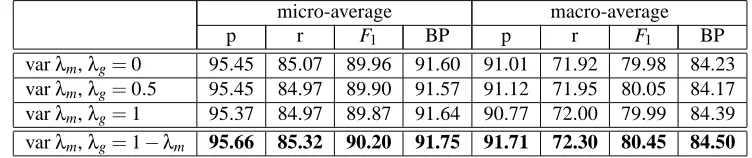
varλm,λg=0 95.45 85.07 89.96 91.60 91.01 71.92 79.98 84.23

varλm,λg=0.5 95.45 84.97 89.90 91.57 91.12 71.95 80.05 84.17

varλm,λg=1 95.37 84.97 89.87 91.64 90.77 72.00 79.99 84.39

varλm,λg=1−λm 95.66 85.32 90.20 91.75 91.71 72.30 80.45 84.50

Table 5: The impact of locality on Precision (p), Recall (r), F1score and Break-even Point (BP). We compare the performance obtained for symbol-dependant decay factors withλg=0 (no gaps allowed),λg=

0.5,λg=1 (any gap allowed) andλg=1−λm(IDF-dependent). All results are for word-sequence

kernels with n=2 and µ=0.5.

The last three rows of Table 4 display the results obtained with IDF (eq. 15) in the polynomial kernels, and with corresponding variableλm(eq. 16) in the word-sequence kernel. By taking word order into account,

the word-sequence kernel yields a better precision, but this does not offset the large gain in recall observed for the standard polynomial kernel, which now performs best overall. These results suggest that taking word order into account does not benefit categorisation performance.

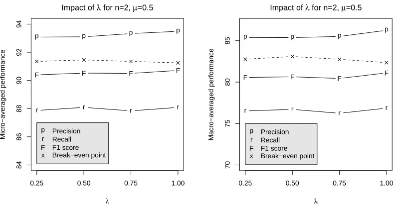
LOCALITY

The decay factorλallows to control the extent to which “gaps” are allowed in matching subsequences. For λ=1, gaps will have no effect on the sequence similarity, while forλ→0, any gap within a subsequence will drive the corresponding feature value (and hence the similarity) towards 0 (cf. eqs. 4 and 5).

The aim of our second experiment is therefore to check the importance of taking into account the distance at which matched words occur, ie whether matches should be local (smallλ) or whether they may occur accross the entire document (largeλ). Note that for symbol-dependent decay factors,λg=0 corresponds to

a pure n-gram model, whileλg=1 is similar to polynomial kernels (with an additional order constraint).

For fixed λ, Figure 3 shows that the setting ofλ has little effect on the performance, suggesting that locality is not overly important for our categorisation task. Table 5 displays similar results for the symbol-dependent decay factors and different settings forλg.

Impact of λ for n=2, µ=0.5

λ

Micro−averaged performance

0.25 0.50 0.75 1.00

84

86

88

90

92

94

p p p p

r r r r

F F F F

p r F x

Precision Recall F1 score Break−even point

Impact of λ for n=2, µ=0.5

λ

Macro−averaged performance

0.25 0.50 0.75 1.00

70

75

80

85 p p p

p

r r

r r

F F F F

p r F x

Precision Recall F1 score Break−even point

Figure 3: The effect of locality (varying decay factorλ) on the performance. All experiments are with n=2 and µ=0.5. The decay factor and hence the number of gaps within a matching subsequence seems to have little impact on performance.

micro-average macro-average

p r F1 BP p r F1 BP

µ=0.5, varλm 95.45 84.97 89.90 91.57 91.12 71.95 80.05 84.17

µ=2, varλm 94.28 88.16 91.12 91.50 89.71 77.27 82.78 83.87

Table 6: The impact of µ on Precision (p), Recall (r), F1score and Break-even Point (BP). We compare the performance obtained for symbol-dependent decay factors with µ=0.5 (more weight to multi-word matches) and µ=2 (more weight to single-word matches).

INFLUENCE OFµ

Parameter µ gives the relative weight of multi-word terms compared to single words. In our experimental results, we focus on µ=0.5, which for n=2 corresponds to giving double weight to matches on two words compared to single-word matches. As mentionned earlier, this allows to emphasize the effect of multi-word matches, but is not necessarily optimal. Indeed, some results in IR suggest that it usually helps to give more weight to single terms with respect to multi-word terms (Gaussier et al., 2000).

Impact of µ for n=2, λ=0.5

µ

Micro−averaged performance

0.25 0.5 1 2

86 88 90 92 94 p p p p r r r r F F F F p r F x Precision Recall F1 score Break−even point

Impact of µ for n=2, λ=0.5

µ

Macro−averaged performance

0.25 0.5 1 2

74 76 78 80 82 84 86 p p p p r r r r F F F F p r F x Precision Recall F1 score Break−even point

Figure 4: The effect of varying the relative weight of multi-terms µ on the performance. All experiments are with n=2 andλ=0.5.

Impact of n for λ=0.5, µ=0.5

n

Micro−averaged performance

2 3 4

80 85 90 95 p p p r r r F F F p r F x Precision Recall F1 score Break−even point

Impact of n for λ=0.5, µ=0.5

n

Macro−averaged performance

2 3 4

55 60 65 70 75 80 85 90 p p p r r r F F F p r F x Precision Recall F1 score Break−even point

Figure 5: The effect of varying the subsequence length n on the performance. All experiments are with µ=0.5 andλm=λg=0.5.

INFLUENCE OFn

INFLUENCE OF SYMBOL-DEPENDENT MATCHING SCORES AND DECAY FACTORS

All experiments show that using symbol-dependentλ’s for matching symbols has a positive influence on performance. As mentioned in Section 4.1, symbol-dependentλ’s allow us to make use of an IDF-based weighting scheme. The fact that this weigthing scheme improves the results comes as no surprise as the importance of IDF based term weighting is well known from the IR literature.

We observe, however, that word-sequence kernels are less sensitive to term weighting than quadratic kernels. Table 4 shows that the performance of the kernel improves when an IDF based weighting scheme is used (fourth line), in particular for the macro-average, but the improvement remains marginal for the micro-average. On the contrary, using IDF yields a significant improvement for the quadratic kernel, both on the micro- and macro-average: the break-even point increases from 87% to 91.74% in micro-average, and from 76.72% to 84.82% in macro-average (Table 4, lines 3 and 6).

COMPARISON OF WORD-SEQUENCE KERNELS WITH OTHER KERNELS

The best performance obtained with word-sequence kernels of length 2 (last line of Table 5) are comparable to the best performance obtained with a polynomial kernel of degree 2 (last line of Table 4). In addition, our results are comparable with state-of-the-art results on this collection using SVM and various bag-of-word kernels.5 Experimental results also show that word-sequence kernels perform better than string kernels on the complete set of documents, when string kernels must be approximated (Lodhi et al., 2002).

Compared to polynomial and RBF kernels, word-sequence kernels have the disadvantage of being com-putationally more demanding. However, as we have seen, word-sequence kernels allowed us to test the importance of different factors for text categorisation, an approach which was not possible before. Lastly, word-sequence kernels rely on several parameters which have been fixed in our experiments, but can in theory be optimised for a specific collection. We will investigate such a tuning in future work.

EXPERIMENTAL RESULTS SUMMARY

In summary, our experiments seem to show the following:

1. Taking word order into account (Table 4) has very little effect on performance. When IDF is applied precision is slightly increased and recall is slightly reduced;

2. Locality per se (Figure 3 and Table 5) has virtually no impact. Some improvement can be obtained by penalising more heavily those non-contiguous word combinations which are obtained by skipping terms with low document frequency;

3. Giving more relative importance to word combinations in the similarity measure increases precision at the expenses of recall (Figure 4 and Table 6);

4. Similarly, considering the combination of more words as indexing terms increases precision at the expenses of recall (Figure 5);

5. Weighting matches according to IDF-basedλm’s improves performance;

6. Finally, the results obtained with word-sequence kernels are comparable to state-of-the-art results on the same collection.

5. New Directions in Word-Sequence Kernels

In the previous section, we defined and illustrated the use of word-sequence kernels, and their extension to symbol-dependent decay factors. We introduce here two additional natural extensions of word-sequence

kernels. These extensions address two linguistically motivated problems: estimating the similarity between documents containing different words with similar meanings (synonyms), or between documents in different languages (cross-lingual).

5.1 Soft Matching

In the standard definition of word-sequence kernels (Sections 2.2 and 4), only exact symbol matches con-tribute to the similarity. One shortcoming of this approach is that synonyms or words with related meanings will never be considered similar. We address this problem by considering soft-matching of symbols, ie match-ing equivalent as well as identical symbols, ensurmatch-ing that matchmatch-ing equivalent symbols contributes less to the similarity than an exact match.

Several IR techniques implement some kind of soft-matching. For example, the Generalised Vector Space Model (GVSM, cf. Wong et al., 1985, Sheridan and Ballerini, 1996) uses the document-term matrix to esti-mate a term-term similarity on the basis of co-occurrences of terms in documents. Similarly, in the context of sequence kernels, we can define a soft-matching extension by invoking a similarity matrix in the implicit feature space:

Ksoft(s,t) =φ(s)>Aφ(t) =

∑

u,v

φu(s)φv(t)Auv (20)

Setting Auv=1 iff u=v, we recover the original formulation. Equation 20 expresses a valid kernel as

long as the similarity matrix A= [Auv]is positive definite. Note that A∈ R+0 Σn_×Σn

is indexed on the feature space dimensions, ie ordered subsequences of length n. In order to simplify the processing and be able to calculate the kernel value without feature space expansion, it may be convenient to express the similarity at subsequence level as a product of similarities at the symbol level: Auv=∏nk=1aukvk. In that case, since A is

the n-fold tensor product of the symbol similarity matrix a= [axy]∈ R+0 Σ×Σ

, A is positive definite whenever a is. The soft-matching word-sequence kernel may be calculated recursively using Equations 6 to 7, 10 and 11, replacing Equations 8 and 9 by the single equation:

K_i00(sx,ty) =λK_i00(sx,t) +λ2axyKi0−1(s,t), ∀x,y,

and modifying Equation 12 to:

Kn(sx,t) =Kn(s,t) +

|t|

∑

j

λ2_a xtjK

0

n−1(s,t[1 : j−1])

Soft matching can be combined with the use of distinct decay factors for gaps and matches:

K_dsn(s,t) = φˆ(s)>A ˆφ(t)

=

∑

u∈Σn_v

∑

_∈Σn_i:u

∑

_=s[i]j:v

∑

_=t[j]

λ2n m

n

∏

k=1

auk,vk

∏

i1<l<in,l6∈i

λg,sl

∏

j1<p<jn,p6∈j

λg,tp (21)

and the recursion formulas can be adapted accordingly.

5.2 Cross-Lingual Document Similarity

LetΣ1andΣ2be two alphabets corresponding to the dictionaries of the two languages under consideration (|Σ1|=m,|Σ2|=q,Σ=Σ1∪Σ2). As a “document” in the parallel collection is actually a pair of aligned documents, we will designate it as a p-document for clarity. In the following, we decompose the p-document-term matrix D into language specific parts D1and D2, such that D= [D1D2].

5.2.1 GENERALISEDVECTORSPACEMODEL

The use of the GVSM in cross-language IR amounts to substitute the original documents with their projection into a dual space, the dimensions of which are induced from clusters of p-documents. In the case where each such cluster contains only one p-document, and using the standard cosine measure, one gets:

KGVSM(d,d0) =cos(D1d,D2d0) =

d>D1>D2d0 kD1dk kD2d0k

(22)

with d in language 1 and d0in language 2. Assuming that raw frequencies are used as term frequencies in the document representation, we can expand the numerator of (22) in the following way:

d>D1>D2d0=

∑

u∈Σ1

∑

v∈Σ2

∑

s:d[s]=ut:d

∑

0[t]=v

(D1>D2)uv

where d[s]corresponds to the term occurring at position s in d (and similarly for d[t]). Lastly, considering the

(m+q)square matrix

A

=D>D=

D1>D1 D1>D2 D2>D1 D2>D2

, we obtain the following symmetric expression:

d>D1>D2d0=

∑

u∈Σv

∑

∈Σs:d

∑

[s]=ut:d

∑

0[t]=v

(

A

)uv (23)

which corresponds to the soft-matching word-sequence kernel (eq. 21) with n=1 andλ2_mauv= (

A

)uv. The

complete cosine similarity is then obtained through standard length normalisation.

5.2.2 CROSS-LINGUALLSI

The cross-language Latent Semantic Indexing model (Dumais et al. (1996)) is similar to the monolingual setting (Deerwester et al. (1990)), except that it is based on the singular value decomposition of the combined p-document-term matrix D. Assuming that we select the dimensions with the highest k singular values, the similarity is calculated after projecting documents using Uk, the(m+q)×k matrix containing the first k

columns of U. Accordingly, the cosine similarity measure for cross-language LSI is given by:

KLSI(d,d0) =cos(Uk>d,Uk>d0) (24)

where documents d and d0are appropriately zero-padded into(m+q)dimensional vectors. In a way similar to how we derived a word sequence kernel for GVSM from Equation 22, we can derive a word-sequence kernel with n=1 for cross-language LSI, provided once again that raw frequencies are used as term frequencies. In this case, the similarity coefficients areλ2_mauv= (UkUk>)uv. Once again, the complete equivalence with the

cosine measure relies on length normalisation.

Note that, to be used in cross-language IR, both GVSM and LSI need a parallel corpus, which is not the case for word-sequence kernels, which can be computed based on a bilingual lexicon derived from a comparable corpus for example.

6. Conclusions

In this paper we first tried to analyse why sequence kernels operating at the character level, with no higher level information, have been so successful. We formulated the noisy stemming hypothesis, according to which sequence kernels perform well because they implicitly select relevant word stems as indexing units. We showed that this hypothesis is supported by empirical observations. Moreover, our observations suggest that the subsequences which are more discriminant are essentially distributed on more than one word stem, and therefore contribute to the effectiveness of the categorisation by indexing pairs of consecutive words.

In this paper we focussed on the word-sequence kernels, where documents are considered as sequences of words. One advantage over the string kernel is that we use more semantically meaningful indexing units. In addition, word-sequence kernels are significantly less computationally demanding. Finally, they lend themselves to a number of natural extensions. We described the use of symbol-dependent decay factors and independent decay factors for gaps and matches in the context of word-sequence kernels. This allows the use of linguistically motivated background knowledge, and of traditional weighting schemes. We showed that the use of independent IDF-based decay factorsλmandλgyields better performance than fixedλ.

The flexibility of word-sequence kernels allowed us to test a number of hypotheses regarding the impact of word order, locality or multi-term matches on the categorisation performance. Our results suggest that order and locality have essentially no effect on the performance, while the length of multi-term matches and their weight in the similarity measure has a clear influence on the precision, recall and F-score.

Finally, we envisioned the possibility of using soft-matching of symbols in order to take into account a similarity between different but related words. This opens up the possibility of using word-sequence kernels in the context of multi-lingual document processing, and apply kernel methods to documents from different languages.

Word-sequence kernels are a particular case of convolution kernels, and our work contributes to the in-vestigation of document representations that are more structured than the bag-of-words model, in the context of IR and document categorisation.

7. Acknowledgements

The work presented in this paper was sponsored by the European Commission through the IST Programme under Contract IST-2000-25431. We are extremely grateful to our partners from the EU KerMIT (Kernel Methods for Images and Text) project for discussing these topics with us. In particular we wish to thank John Shawe-Taylor for many comments and suggestions for possible extensions of the word-sequence kernel, and Craig Saunders for help with the string kernel experiments. We also acknowledge many insightful comments from the anonymous reviewers.

Appendix A. Recursive Formulation of Sequence Kernels

This appendix gives an intuitive description of the basic sequence kernel, as well as a derivation of an efficient recursive formulation based on dynamic programming.

We first recall some basic notation and definitions:

LetΣbe a finite alphabet, and let s=s1s2···s|s|be a sequence over such alphabet (i.e. si∈Σ,1≤i≤ |s|).

Let i= [i1,i2,...,in], with 1≤i1<i2< ... <in≤ |s|, be a subset of the indices in s: we will indicate as

s[i]∈Σnthe subsequence si1si2...sin. Let us write l(i)the value in−i1+1, i.e. the length of the window in s

spanned by s[i].

The basic Sequence Kernel works in the feature space of all possible subsequences of length n, where the value associated with the feature u is defined by:

φu(s) =

∑

i:u=s[i]

λl(i) ₍₂₅₎

matching symbols. For instance, ifλis given the value 1, the gaps are not taken into account when computing the value of the featureφu(s). Whenλis given the value 0.5, each gap symbol contributes to dividing the

feature value by 2 (without gap,φu(s) = (0.5)n).

The sequence kernel of two strings s and t overΣis defined as the inner product:

Kn(s,t) =

∑

u∈Σn

φu(s)·φu(t) =

∑

u∈Σn_i:u

∑

_=s[i]

λl(i)

∑

j:u=t[j]

λl(j)₌

∑

u∈Σn_i:u

∑

_=s[i]j:u

∑

_=t[j]

λl(i)+l(j) ₍₂₆₎

Intuitively, this means that we match all possible subsequences of n symbols, with each occurrence “discounted” according to the size of the window that it spans. Consider for example the alphabetΣ=

{A,C,G,T}, and the two elementary sequences:

s=CAT G and t=ACAT T

For n=3, the weights of all subsequences (or features) for sequences s and t are, according to (25):

u φu(s) φu(t) u φu(s) φu(t)

AAT 0 λ4+λ5 CAG λ4 0

ACA 0 λ3 _CAT λ3 λ3₊λ4

ACT 0 λ4+λ5 CTG λ4 0

ATG λ3 0 CTT 0 λ4

ATT 0 λ3+λ5 others 0 0

where for instance the value of the feature u=AAT for sequence t=ACATT isλ4+λ5because there are two occurrences of AAT in ACATT. The first spans a window of width four (first, third and fourth symbols) and the second spans a window of width five (first, third and fifth symbols). The similarity score is then:

K3(CAT G,ACAT T) =hφ(s),φ(t)i=

∑

u

φu(s)φu(t) =λ3(λ3+λ4)

as the only feature for which both sequences have a non-null value is CAT.

A direct computation of all the terms under the nested sum in (26) becomes impractical even for small values of n. In addition, in the spirit of the kernel trick discussed in Section 2, we wish to calculate Kn(s,t)

directly rather than to perform an explicit expansion in feature space. This can be done using a recursive formulation proposed by Lodhi et al. (2001), which leads to a more efficient dynamic-programming imple-mentation. The recursive formulation is based on the following reasoning. Suppose that we already know the value of the kernel for two strings s and t: what do we need to compute the value of the kernel for sx and t, for some x∈Σ? Notice that:

1. All subsequences common to s and t are also common to sx and t.

2. In addition, we must consider all new matching subsequences ending in x which occur in t and whose (n-1)-symbol prefix occur in s (possibly non-contiguously).

For the latter point, consider the example in Figure 6. Let u0 and u00 be two distinct sequences of length n−1. They occur in both s and t and, as occurrences can contain gaps, each occurrence spans, in principle, a window of different length. Let’s focus, for instance, on the occurrence of u00in s marked as a. If iais the set of indices of the occurrence, i.e. if u00=s[ia], then the length of the window spanned by the occurrence is ia_n−1−ia₁+1. The occurrence a will give raise to two new matches of length n for the subsequence u00x between sx and t, due to the presence of the occurrence of u00marked as b in t and to the two occurrences of x to the right of b in t. These two matches will contribute to the kernel according to their lengths:

λ2_(λ|s|−ia

1+1λjl1−j1b+λ|s|−ia1+1λjl2−jb1)

where jbis the set of indices of b in t, and jl1and jl2are the indices of the relevant occurrences of x in t, as