International Dotorate Shool in Information and
Communiation Tehnologies
DIT - University of Trento
Multi-Resolution Tehniques based on
Shape-Optimization for the Solution of Inverse
Sattering Problems
Manuel Benedetti
Thesis ino-tutelle between University of Trento (Italy)
and Université Paris Sud XI (Frane).
Thesis with European Label.
Advisor:
Andrea Massa, Professor
Università degli Studi di Trento
Co-Advisor:
Dominique Lesselier,Direteur de Reherhe
Laboratoiredes Signauxet Systèmes (Supéle-CNRS-UPS)
SPECIALITE: PHYSIQUE
Eole Dotorale Sienes et Tehnologies
de l'Information des Téléommuniations
et des Systèmes
Présentée par Manuel Benedetti
Sujet:
TehniquesMulti-Résolutionbaséessurl'Optimisation
de FormepourlaRésolutionde ProblèmesInverses
de Diration
Thèse en o-tutelle entre Université de Paris Sud 11 (Frane)
et University of Trento (Italie). Thèse ave lelabel européen.
Soutenuele1 er
Deembre2008devantlesmembresdujury:
M.LESSELIER Dominique
M.MASSA Andrea
M.DORN Oliver
M.PICHOT Christian
Arriving at the end of my Ph.D., I would like to express my
gratitude to all those who gave me the possibility of arrying
out suh a wonderful professional experiene. First of all, I
want to thank my thesis advisors Andrea Massa, Professor of
Eletromagneti Fields at the University of Trento and
Dire-tor of the Eletromagneti Diagnosti Laboratory (ELEDIA
Lab.), andDominique Lesselier,Direteurde Reherhe atthe
Laboratoiredes SignauxetSystèmes (L2S)ofSupéle,whohad
ondene in my abilities as well as in the o-tutelle program
in whih I was involved.
My speial thanks also go to my tutors Mar Labert,
re-searher at L2S, and Massimo Donelli, researher at the
Uni-versityofTrentoandmemberoftheELEDIAgroup. Certainly,
I will never forget their helpfulness in providing me with so
many theoretial suggestions as well as with useful tips at a
more pratiallevel.
Moreover,Iwanttothankallmydearolleaguesandfriends
oftheELEDIAResearhGroup,whoseskillsandkindness
on-tribute tomakethe Ph.D.a great professionalexperieneand
a wonderful life experiene at the same time. I amdeeply
in-debted to all of them, stritly in alphabetial order by name
(I hope not to forget anybody), Andrea Rosani, Anna
Mar-tini, Aronne Casagranda, Davide Franeshini, Edoardo Zeni,
Aramini.
I also have to thank for the kindness the olleagues and
friends that I met during my stays at L2S, to be more
pre-iseAndreaCozza,AnthonyBourges,ArnaudBreard,Bernard
Duhene,ChinYuanChong,ChristopheConessa,CyrilDahon,
Frédéri Brigui, Frédéri Nouguier, Houmam Moussa,
Jean-Philippe Groby, Juan Felipe Abasal, Karim Louertani,
Nio-las Ribiere-Tharaud, Tommy Gunnarsson, and Rami Kassab.
A speial thank goes to the administrative sta of the lab as
well,namely Daniel Rouet and Maryvonne Giron.
Finally, I aminnitely grateful tomy family,Stefano,
Pie-rina, Susanna, and Miòl, whose patient love and
In the framework of inverse eletromagneti sattering
teh-niques, the thesis fouses on the development and the analysis
of the integration betweena multi-resolution imaging proedure
andashape-optimization-basedtehnique. Thearising
method-ologyallows,ononehand,tofullyexploitthelimitedamountof
informationolletablefromsattering measurements bymeans
of the iterative multi-saling approah (IMSA) whih enables
a detailed reonstrution only where needed without
inreas-ing the number of unknowns. On the other hand, the use of
shape-optimization, suh as the level-set-based minimization,
providean eetive desription of the lass of targets to be
re-trieved by using a-priori information about the homogeneity
of the satterers. In order to assess strong points and
draw-baks of suh an hybrid approah when dealing with one or
multiple satterers, a numerialvalidation of the proposed
im-plementations is arried out by proessing both syntheti and
laboratory-ontrolled sattering data.
Keywords
La reonstrution non invasive de la position et de la forme
d'objets inonnus onstitue un thème de grand intérêt dans
nombred'appliations,etoniteraenpartiulierl'évaluationet
le ontrle non destrutif(généralement référés par les
abrévi-ations END et CND)pour lasurveillane etle ontrle
indus-triel etle diagnosti de sous-surfae [1℄. Dans un tel adre
in-téressant, beauoup de méthodologies ont été proposées,
prin-ipalement basées sur les rayons X [2℄, les ultrasons [3℄, et les
ourantsdeFouault[4℄. Cependant,desapprohesdansle
do-mainemiroonde(parlequelonentendde300MHzà300GHz)
ontétéréemmentreonnues ommeorantdes méthodologies
d'imagerie eaes, grâe aux points lés suivants[1℄[5℄[8℄ :
•
les ondes életromagnétiques aux fréquenes miroondespeuvent pénétrer matériaux naturels et artiiels sous
réserve qu'ilsne soient pas des onduteurs idéaux ;
•
leshampsdiratésparleoulesobjetsiblessontrepré-sentatifsnonseulementdes frontièresdeelui-iou
•
les miroondes montrent une grande sensibilité auon-tenueneaudelastruturequel'onentreprendd'imager;
•
les sondes de e domaine peuvent être employées sansauun ontat méanique ave le spéimen testé .
De plus, en omparaison aux rayons X voire aux approhes
basées sur la résonane magnétique, les méthodes miroondes
minimisent(ouévitent)deseets ollatérauxdans lespéimen
testé. Don, elles peuvent par exemple être mises en ÷uvre
de manière plus sûre en imagerie biomédiale, en limitant
en-tre autre le stress du patient dans la mesure où le ontat
physique ave le système d'imagerie peut être évité (e.g., le
dépistagede aners dusein [9℄),oudansd'autresappliations
ritiques,tellesquel'imagerieàtraverslesmurs(dite
Through-WallImaging ouTWI) [10℄.
Une avanée supplémentaire de l'inspetion non invasive
miroondeest représentée par des approhes de diration
in-versequisontdestinéesàonstruireuneimagedelarégionsous
test qui ontiennent de l'informationquantitative bien dénie
[11℄. Laformulationmathématiquedu problème de diration
inverse est présentée auhapitre 2en seonentrant surle as
où des informations a priori sur la géométrie sont
eetive-mentdisponibles. Puisque lesproblèmes de dirationinverse
n'ontgénéralementpasunesolutionsousuneformeanalytique,
une résolution numérique basée sur la méthode des moments
(MoM) est adoptée et lesinonvénients prinipaux du modèle
qui apparaissent, tels que la non linéarité, le mauvais
alors que la non linéarité est due au fait que la solution ne
peut pas être exprimée ommeune sommelinéaire d'éléments
indépendants. Par suite de la mauvaise loalisation, le
prob-lème inverse soure également de mauvais onditionnement,
puisque la solutionne dépend pas en ontinuité des données.
An de disuter les stratégies de résolution qui ont été
développéespour surmonterdetelsinonvénients,lehapitre3
seonentresurlasituationatuelledansleadredela
dira-tion inverse. En partiulier, lessolutionsrégularisées [38℄
on-sistent à exprimer quelques propriétés physiques prévues des
dirateurs au moyen de paramètres de régularisation, de e
fait onstruisant une famille de solutions approhées.
Mal-heureusement, lehoixdu oudes paramètres de régularisation
devient alors le thème prinipal, partiulièrement dans le as
des problèmesnonlinéairespourlesquelslalittératurene
four-nit auun ritère. De façon analogue, l'utilisationdes
approx-imations, telles que Born, Rayleigh et Rytov [13℄, est limitée
à une lasse spéique des problèmes de diration inverse,
'est-à-dire traitantlesdirateurs de faiblesontrastes.
Àladiérenedestehniquesetapproximationsde
régular-isation,lestehniquesdeminimisationtententdefairefaeàla
non-linéaritéduproblèmededirationinverse. Ces
méthodolo-giesreformulentleproblèmeommeuneproédured'optimisation
visantà laminimisationde l'éartentre leshampsmesurés et
la solution d'essai numériquement alulée. À et eet, une
fontion de oûtappropriée est dénieetl'espaede reherhe
ef-l'eaitéde lastratégiedesolution,puisqueleproblème peut
posséderdessolutionserronéesde parsanon-linéarité. Dansle
adre de stratégies de minimisation, la thèse dérit stratégies
déterministes et heuristiques de minimisation. Les plus
large-mentonnuespourlapremièreatégoriesontlesméthodologies
baséessurdesminimisationspardesenteselonlegradientainsi
que présentées par Kleinman et al. [54℄. Ces méthodologies
sontbasées sur ladénitiond'une sériede solutionsd'essai
as-soiéesàdesvaleursstritementdéroissantesde lafontionde
oûtetellessontaratériséesparlamiseàjourduhamp
éle-trique inonnuainsiquedes valeursdes propriétés
életromag-nétiques (i.e., permittivité diéletrique et ondutivité) dans
le domainede reherhe. Malheureusement, la onvergene de
la minimisation déterministe dépend du point d'initialisation,
puisque lasolutionpeut être bloquée à desminima loaux par
suite de la non-linéarité du problème. Au ontraire, les
teh-niques heuristiques peuvent limiter le probléme de minima
lo-aux grâe à leur apaité d'explorer l'espae de reherhe en
totalitéainsiqueàlapossibilitéd'inluredel'informationa
pri-ori dans la solution. Une telle lasse de stratégies de
minimi-sation se ompose généralement d'algo-rithmes stohastiques
inspirés du omportement d'insetes pour la mise à jour des
inonnues.
Sans élaborer au delà du néessaire à e stade, le
ara-tère malposé est fortement liéàlaquantité d'informationque
l'on peut olleter lors d'une expériene de diration à but
d'imagerie, et habituellement le nombre de données
vironnant la zone étudiée) ou/et à illumination multiple (on
élaireettezone d'étudede plusieurs diretionsouàpartirde
souresréparties dans plusieurs domaines)sont don
générale-ment adoptés. Cependant, il est bien onnu quel'information
qui est eetivement aessible par e ou es moyens est une
quantité qui onnaît une limite supérieure [14℄[15℄. En
on-séquene, ilest néessaire d'exploiterde manièreeae toute
l'informationontenuedansleséhantillonsreueillisduhamp
diratéan d'atteindreunereonstrution (d'obtenirune
im-age) qui soit satisfaisante. Comme disuté dans le hapitre
3, an d'exploiter eetivement toute l'information olletée
à partir des mesures de diration eetuées, des stratégies
dites de multi-résolution ont été réemment proposées. L'idée
est de viser une résolution spatiale performante ('est-à-dire
améliorée par rapport à elle ouramment hoisie ou assurée
dans lazoned'étude) seulementdanslesrégionsd'intérêt
(Re-gions of Interest dites RoIs) de l'espae oû les dirateurs
in-onnussontloalisés(pluspréisément,oûilssontestimésêtre
par le proessus d'imagerie qui est mis en ÷uvre) [16℄ et/oû
des disontinuités entre matériaux apparaissent être présentes
[17℄[18℄. Quantauxréalisationspratiques,desstratégies
déter-ministes ou impliquant des analyses statistiques des données
ont été proposées an de déterminer le niveau de résolution
optimal, tandis que des approhes impliquant des fontions
splines de degrés variés ont été employées an d'améliorer le
niveau de résolution. Par ailleurs, des approhes multi-étapes
itéra-à elle d'un zoom [19℄ en gardant le rapport entre le nombre
d'inonnues(e.g.,lesparamètreséletromagnétiquesdeellules
ave lesquelles on onsidère quela zone d'étude est divisée) et
le nombre de données (e.g., les éhantillons reueillis du ou
des hampsdiratés) susamment faibleet onstant de telle
façonquelerisquedelasurvenuedeminimaloauxd'une
fon-tionnelle oût (qui traduit de manièreusuelle l'éart entre les
données et elles que l'on pourrait assoier par la simulation
numérique aux objets modélisés par la proédure d'inversion,
etqui orrespond au moins indiretementà ladiérene entre
lesobjetsréelseteuxquinousapparaissentreonstruits)dans
le problème d'optimisationtelque onsidéré [15℄.
Par ailleurs, l'absene d'information aetant la bonne
ré-solutiondu problèmeinverseaétéonsidérée,partiulièrement
enEND-CND, àtraversl'exploitationdelaonnaissanea
pri-ori que l'on peut avoir sur la sène de test, et du sénario
de l'interation életromagnétique misen jeu, aumoyen d'une
représentationeae des inonnues de elle-i. Eneet, dans
beauoup d'appliations, le oules objets inonnus sont
ara-tériséspardespropriétéséletromagnétiquesonnues(i.e.,
per-mittivité diéletriqueet ondutivité)et ilssontloalisésdans
une régionhte onnue aumoinsàunertaindegré(des
iner-titudes peuvent l'aeter, ei menant à une omplexité
addi-tionnelle qui pourrait être signiative). De plus, ela
dépen-dant de la préision reherhée, des sénarii plus omplexes
peuvent êtreapprohés vial'introdutiond'un ensemblede
ré-gionshomogènesaratériséespardesparamètresgéométriques
lequelesontlessupportsdeesrégionshomogènesquidoivent
être reonstruits. An d'atteindre un tel but, des tehniques
paramétriques qui sontdestinées à représenter l'objet inonnu
en terme de paramètres desriptifs de formes de référene [21℄
[22℄,desapprohesplussophistiquéestellesquel'évolution
on-trlée de ourbes de type splines [23℄[25℄, des gradients de
forme [26℄[28℄, ou des méthodes d'évolution d'ensembles de
niveaux [31℄[32℄, ont été proposées. Plus en détail, quant aux
stratégies d'optimisation de forme les plus importantes dans
la formation d'images en miroonde (le hapitre 4), des
ap-prohes paramétriquessontbaséessurladesriptiondesobjets
aumoyendeformesdebasequisontorretementparamétrées.
Pour e qui onerne les méthodes d'ensembles de niveaux, le
ontour zéro d'un tel ensemble dénit la frontière du ou des
objets homogènes reherhés, e qui, en ontraste aux
straté-giesquiimpliquentunedesriptionenpixelsouparamétriques,
permet de représenter des formes omplexes ou des régions
d'une manière relativement simple (on parlera de méthodes
d'inversion libres de ontraintes topologie). De plus, à la
dif-férene des approhes paramétriques, les ensembles de niveau
permettentdeontrlerlafusionetladivisiondesobjetsd'une
manière naturelle.
Dans le adre brossé i-dessus, la thèse se foalise sur le
développementetl'analysedel'intégrationd'unestratégie
multi-éhelleitérative(diteIterativeMulti-SalingApproahouIMSA)
[19℄ et de la représentation en ensembles de niveaux
ori disponible sur le sénario joué (e.g., l'homogé-néitédu ou
des dirateurs en est le point lé) que le ontenu informatif
des mesures eetuées. Par raison de simpliité, et sans
pré-tention à exhaustivité, la formulation du problème inverse est
réduite au as bidimensionnel de polarisationtransverse
mag-nétique (TM) quand on traitera d'une oude plusieurs régions
d'intérêt.
En partiulier, l'arhiteture de la stratégie proposée est
présentée au hapitre 4. La formulation mathématique de
l'approheitérativemulti-résolutionavelaminimisationbasée
sur l'ensemble de niveaux (notée IMSA-LS)est onentrée sur
l'arhiteturemulti-étape. L'algorithmeestbasésurdesétapes
où la résolution spatiale est itérativement augmentée en
on-entrantlarégiond'intérêtsurleseteuroùl'objetestloalisé.
À la première étape, le domaine de reherhe est disrétisé et
unesolutionbruteest reherhée. Puis, àpartirdelapremière
évaluation,lapremière régiond'intérêtestestiméeetleniveau
de résolution est augmenté seulementà l'intérieurde larégion
d'intérêt. À et eet, une nouvelle fontion multi-résolution
d'ensemble des niveaux est dénie et son évolution est menée
enrésolvantunproblèmeadjointquiorrespondàladérivation
de la fontion de oût.
L'évaluation des possibilités de reonstrution d'IMSA-LS
est eetuéepremièrement en onsidérant des géométries
sim-ples, telles qu'un ylindre irulaireave un rayonde la
demi-longueurd'onde,etdesdonnéessynthétiques. L'algorithmeest
initialiséavelasolutionvraieanderéaliserunessaide
uté. Enoutre,l'exéution proposéeest omparéeàl'approhe
dite "bare", 'est-à-dire la méthode standard. Généralement,
l'IMSA-LS semble être plus préis partiulièrement ave de
faibles rapports signal à bruit. Les mêmes onlusions
tien-nentégalementenonsidérantdesformesplusomplexes,telles
que leylindre retangulaire oule ylindrereux. Pour mieux
investiguerl'évaluation,des données aquisesen situation
on-trlée de laboratoire pour quelques géométries d'essai ont été
aussi onsidérées. Dans de telles expérienes, IMSA-LS et
l'approhe"bare"fournissentdesrésultatssimilairesen termes
d'exatitude, puisque es données sont probablement aetées
par un faibleniveau du bruit.
Le hapitre 5 se onentre sur un développement ultérieur
de l'IMSA-LS, aratérisé par la possibilité de traiter des
ré-gions d'intérêt multiples, partiulièrement pour reonstruire
plusieurs objets de façon plus eae en termes d'attribution
des inonnues. Plus en détail, une telle stratégie, appelée
IMSMRA-LS,estaratériséeparunearhiteturemulti-étape,
où à haque niveau de résolution diérentes régions d'intérêt
sont prises en onsidération simultanément. À la première
étape, un problème "bare" est résolu en hoisissant le
nom-bre de domaines selon la quantité d'information indépendante
dans lesdonnées diratées[14℄. Puis, àpartirdes évaluations
brutes des objets, les régions d'intérêt sont dénies au moyen
d'unestratégieadaptéeànos besoins,baséesur l'identiation
des ontours des formes reonstruites. La résolution spatiale
fra-de maintenir le nombre d'inonnues limité pendant la
proé-dured'inversion. Lareonstrutionmulti-résolutionestréitérée
jusqu'àe quelesparamétresdes régionsd'intérêt,'est-à-dire
leurs baryentres etleurs dimensions, deviennent onstants.
Le hapitre 5 disute également la performane de
reon-strution de l'implémentation multi-région. An de omparer
l'exatitude de lareonstrution fournie par IMSMRA-LS aux
résultats de l'approhe ave une seule région, une validation
préliminaire prend en onsidération un dirateur simple, tel
qu'un ylindre irulaire ave un rayon de la demi-longueur
d'onde, situé dans un domaine arré de té deux longueurs
d'onde. Dans une telle expériene, l'IMSMRA-LS s'avère plus
eaequel'IMSA-LS,partiulièrementenraisondel'utilisation
d'une stratégie de mise à jour de l'ensemble de niveaux plus
appropriée. Après la disussion du hoix des paramètres pour
le ritère d'arrêt, e hapitre 5 propose quelques expérienes
numériquesaratériséespardesdirateursmultiples,telsque
deux ylindres irulaires, deux retangles, ou trois objets de
diérentes formes. Danstouteses expérienes, l'IMSMRA-LS
fournitunereonstrutionlégèrementpluspréisequel'approhe
"bare", alors que l'exatitude des résultats de l'IMSA-LS est
raisonnablement inférieure en raison de la résolution spatiale
plus élevée. Cependant, en onsidérant des formes plus
om-plexes, telles que les ylindres reux et des roix, aussi bien
que des données bruitées, l'IMSMRA-LS surpasse l'approhe
"bare". La dernière illustration onsidérée a trait à la
reon-strution réalisée en traitant des données expérimentales de
résultats tout à fait similaires à eux de la méthode ave une
seule région, puisque les données expérimentales sont
ara-térisées par des rapports signal à bruit élevés. Cependant, en
e qui onerne le dernier as du hapitre 4, l'IMSMRA-LS
sembleêtre plus préisen estimant laformedes ibles.
Enonlusion,etravailproposel'intégrationentre
l'appro-he multi-éhelle et une méthode d'ensemble de niveaux an
d'exploiterde manièreprotable laquantité d'information
ob-tenue vialesmesuresde ladirationaussi bienque
l'informa-tion disponible a priori sur leproblème onsidéré. Deux
réali-sations sontprésentées an de traitereetivement des
ong-urationsaratériséespar unouplusieursobjets. Leséléments
prinipaux de l'approhe peuvent être réapitulés omme suit
:
•
représentationinnovatriemulti-niveaudesinonnuesduproblème dans la tehnique de reonstrution basée sur
les ensembles de niveaux ;
•
limitationdu risque de bloageen des solutionserronéesgrâe aurapportréduit entre données etinonnues ;
•
exploitationutiled'informationsapriori(i.e.,homogénéitéd'objets) sur le sénarioà l'essai ;
•
résolution spatialeaugmentée seulementdans lesrégionsposée, les onlusions suivantes peuvent être tirées :
•
l'IMSA-LS s'est habituellement avéré plus eae quel'approhe "bare", partiulièrement en traitantdes
don-néesbruitéesdiratéesparunobjetde géométriesimple
aussi bien que omplexe;
•
l'IMSMRA-LSasembléêtre aussieae quel'approhe"bare" en traitant des géométries simples, alors qu'une
arhiteture multi-région appropriée a amélioré
l'exati-tude de la reonstrution ave lesdiuseurs multiples;
•
les stratégies intégrées (i.e., IMSA-LS et IMSMRA-LS)ont semblé néessiter moins de aluls que l'approhe
standard, en atteignant une reonstrution possédant le
même niveau de rêsolution spatiale dans la desription
A Two-Step Inverse Scattering Procedure for the
Qualitative Imaging of Homogeneous Cracks in
Known Host Media—Preliminary Results
Manuel Benedetti, Massimo Donelli, Dominique Lesselier, and Andrea Massa
, Member, IEEE
Abstract—
In the framework of nondestructive evaluation and
testing, microwave inverse scattering approaches demonstrated
their effectiveness and the feasibility of detecting unknown
anom-alies in dielectric materials. In this letter, an innovative technique
is proposed in order to enhance their reconstruction accuracy. The
approach is aimed at first estimating the region-of-interest (RoI)
where the defect is supposed to be located and then at improving
the qualitative imaging of the crack through a level-set-based
shaping procedure. In order to assess the effectiveness of the
pro-posed approach, representative numerical results concerned with
different scenarios and blurred data are presented and discussed.
Index Terms—
Genetic algorithms, level set, microwave imaging,
nondestructive testing and nondestructive evaluation (NDT/NDE).
I. I
NTRODUCTION
N
ONDESTRUCTIVE testing and nondestructive evaluation
(NDT/NDE) techniques are aimed at detecting unknown
defects and other anomalies buried in known host objects by
means of noninvasive methodologies [1]–[3]. In such a
frame-work, electromagnetic inverse scattering approaches can play an
important role. As an example, some approaches that
approxi-mate defective regions with rectangular shapes have been
pro-posed [4], [5]. Despite the satisfactory results, such techniques
are adequate when facing NDE/NDT problems where the
re-trieval of the positions and the rough estimation of the sizes of
the defects are enough, but they cannot be reliably used when an
accurate knowledge of the shapes of the defects is needed as in
some industrial processes and usually in biomedical diagnosis.
Notwithstanding, they are useful for providing a “first-step”
in-formation concerned with a rough localization of the defects to
be further improved by means of a successive refinement
recon-struction carried out with suitable contour detection methods.
Towards this end, this letter presents a two-step procedure
aimed at improving the reconstruction of [4], [5]. More in
de-tail, starting from the knowledge of the scattered field with and
without the defect, the approximate problem in which the defect
Manuscript received July 16, 2007; revised October 9, 2007.
M. Benedetti, M. Donelli, and A. Massa are with the Department of
Infor-mation and Communication Technology, University of Trento, 38050 Trento,
Italy (e-mail: [email protected]; [email protected];
D. Lesselier is with the Département de Recherche en
Électromagnétisme-Laboratoire des Signaux et Systèmes, CNRS-SUPELEC-UPS 11, 91192
Gif-sur-Yvette CEDEX, France (e-mail: [email protected]).
Color versions of one or more of the figures in this letter are available online
at http://ieeexplore.ieee.org.
Digital Object Identifier 10.1109/LAWP.2007.910954
is assumed of simple shape (e.g., a rectangle) is reformulated in
terms of an inverse scattering one and successively solved by
means of the minimization of a suitably defined cost function
[6]. After such a step, the region-of-interest (RoI) where the
de-fect is supposed to be located is determined and the second
re-trieval phase takes place by applying a shape-based optimization
technique based on the numerical evolution of a level-set
func-tion [7].
The outline of this letter is as follows. The mathematical
for-mulation of the proposed approach is presented in Section II
by focusing on the second step of the reconstruction procedure.
Then, the effectiveness of the approach is discussed with
refer-ence to a set of representative numerical results in dealing with
blurred measurement data (Section III). Finally, some
conclu-sions follow (Section IV).
II. M
ATHEMATICAL
F
ORMULATION
Let us consider a 2-D scenario where a homogeneous defect
(or crack) characterized of unknown position
and
shape
lies in a cylindrical host region
characterized by
known relative permittivity
and conductivity
. The
de-fective host medium is probed by
electromagnetic transverse
magnetic (TM) plane waves with an incident field
, and the induced electromagnetic field
is given
by
(1)
where
is the free-space Green’s function and
is the object function ( being the working
frequency), or analogously, in a more “practical” expression [8]
(2)
by considering the inhomogeneous Green’s function
and the total electric field in the scenario without defects
defined as follows:
(3)
where
is the differential object given by
if
if
(4)
BENEDETTI
et al.
: TWO-STEP INVERSE SCATTERING PROCEDURE FOR THE QUALITATIVE IMAGING OF HOMOGENEOUS CRACKS
593
With reference to the “differential formulation,” the first step
of the approach considers the partitioning of
in
and the
only one computation of the inhomogeneous Green’s matrix
of
entries according to the procedure detailed
in [8]. Then, the RoI
is modeled with a rectangular
homo-geneous shape described through the coordinates of the center
, its length
, its side
, and the relative
ori-entation
. Accordingly,
turns out to be fully described by
means of the following object function profile:
if
and
otherwise
(5)
where
and
. Under these assumptions, the
unknown array
(6)
is determined by solving the inverse scattering problem
formu-lated in terms of an optimization one.
In detail, starting from the knowledge of the data samples
collected in the observation domain
(i.e., the total field
with the defect
and without the defect
,
) and in the investigation domain
(i.e.,
,
),
is obtained by minimizing the
mismatching between estimated and measured scattering data
evaluated through the computation of
, as shown in (7)
at the bottom of the page. As far as the minimization process
is concerned,
trial solutions
are randomly initialized (
,
being the iteration
index) and an iterative procedure takes place until a
stop-ping criterion holds true (
or
,
). At each
iteration, the following operations are performed:
1) the iteration index is updated
;
2) a set of genetic operators described in [5] is applied to
in order to generate the th
;
3) the
best
trial
solution
achieved
so
far,
being
, is stored and its fitness
evaluated
in order to check the threshold
condition for the stopping criterion.
At the end of the first step, the genetic algorithm (GA)-based
optimization returns the array
that defines the RoI
(8)
where the superscript denotes the estimated values.
The second step of the approach is aimed at refining the
esti-mate of the defect starting from the knowledge coming from the
first step (i.e., the homogeneous defect lies in
). Towards this
purpose, a level-set-based strategy is employed. The algorithm
is initialized by defining an elliptic trial shape
centered at
, with axes equal to
and
, respectively, and
ro-tated by
. Then, the level set
is defined in
according
to the rule based on the oriented distance function [9]. In
par-ticular,
is equal to
if
,
and
otherwise,
being a point
be-longing to the contour of
[7], [9]. Concerning the numerical
implementation,
is discretized in
cells and the following
sequence is iteratively applied.
1) The accuracy of the current trial shape
in retrieving the
actual shape of the defect is evaluated by computing the
value of the metric shown in (9) at the bottom of the page,
where
is the differential object function equal to
if
and 0
(7)
otherwise. Furthermore,
is the solution of the
following equation:
(10)
2) The level-set-based process ends if a fixed number of
it-eration is performed
or
and
is assumed as the crack profile. Otherwise, the level
set function
is updated
by solving a
Hamilton–Jacobi equation
(11)
where
stands for the numerical
counter-part of the Hamiltonian operator [9], [10] and
is the
time-step parameter chosen according to the Courant–
Friedrich–Leroy condition [11]. Moreover,
is
the velocity function determined by solving the adjoint
problem as detailed in [7] and [9].
III. N
UMERICAL
A
NALYSIS
This section is devoted to a numerical analysis of the
pro-posed approach. A set of selected and representative numerical
results related to a couple of experiments are reported and
dis-cussed for pointing out the improvement in the crack detection
and shaping.
The first experiment (indicated as the “experiment A”)
con-siders an unknown void defect of elliptical cross section that lies
in a square lossless host medium of side
and
charac-terized by a dielectric permittivity equal to
. The defect
is located at
and rotated by
with
axes equal to
and
, respectively. The scenario has
been probed by
orthogonal and equally spaced angular
directions and the field has been measured at
points.
Moreover, the scattering data have been blurred with an additive
noise of Gaussian-type characterized by a fixed signal-to-noise
ratio (SNR).
Concerning the numerical procedure,
has been discretized
in
and
in
subdomains.
As an example, Fig. 1(a) shows the reconstruction result from
the two-step procedure in correspondence with SNR
10 dB.
As it can be observed, the support of the defect (whose actual
perimeter is evidenced by the dotted line) belongs to the RoI
(dashed–dotted line) estimated at the end of the first step.
How-ever, the crack dimension is largely overestimated. On the
con-trary, the shape of the crack is more faithfully retrieved, despite
the nonfavorable SNR. Such an event is quantitatively
quanti-fied by the value of the localization error
1.2% [12] that
improves by 30% with respect to the single-step inversion. For
comparison purposes, Fig. 1(b) shows the reconstruction
ob-tained by the “bare” level-set method setting
and
dis-cretizing the domain such that the spatial resolution is equal
to that of Fig. 1(a). As it can be noticed, the reconstruction
worsens.
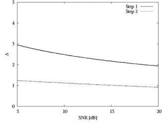
As far as the area error
[12] is concerned, Fig. 2 shows
the behavior of the error figure versus the SNR. As it can be
noticed, the two-step approach turns out to be more robust than
Fig. 1. Experiment A: (a) reconstruction after the first step (i.e., the RoI
)
and dielectric distribution estimated at the end of the two-step procedure;
(b) dielectric distribution estimated by means of the “bare” level set approach
(i.e.,
).
Fig. 2. Experiment A: area error versus SNR.
the blurring on data and the resulting performances are better in
an amount between 150% and 100%.
BENEDETTI
et al.
: TWO-STEP INVERSE SCATTERING PROCEDURE FOR THE QUALITATIVE IMAGING OF HOMOGENEOUS CRACKS
595
Fig. 3. Experiment B: (a) reconstruction after the first step (i.e., the RoI
)
and dielectric distribution estimated at the end of the two-step procedure;
(b) dielectric distribution estimated by means of the “bare” level-set approach
(i.e.,
).
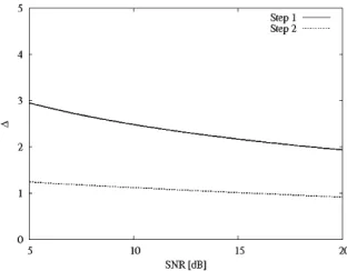
RoI, the two-step approach provides a satisfactory
reconstruc-tion improving both the localizareconstruc-tion error and the area error with
respect to the first step (
1.5%,
0.5%;
3.7%,
1.5%). Similar considerations hold true when smaller
SNRs are considered, as pointed out by the values of the area
error pictorially reported in Fig. 4.
IV. C
ONCLUSION
In this letter, an innovative two-steps procedure for NDE/
NDT applications has been proposed and preliminarily
as-sessed. The method consists of a first step aimed at determining
the region of interest where the defect is supposed to be located
and a successive shaping process for enhancing the qualitative
imaging. The approach has been evaluated by considering
Fig. 4. Experiment B: area error versus SNR.
blurred synthetic data and different crack cross sections. The
achieved results have pointed out the effectiveness of the
ap-proach, thus suggesting its future employment in biomedical
imaging.
R
EFERENCES
[1] P. J. Shull
, Nondestructive Evaluation: Theory, Techniques and
Appli-cations
.
Boca Raton, FL: CRC Press, 2002.
[2] R. Zoughi
, Microwave Nondestructive Testing and Evaluation
.
Am-sterdam, The Netherlands: Kluwer, 2000.
[3] J. C. Bolomey, “Recent European developments in active microwave
imaging for industrial, scientific and medical applications,”
IEEE
Trans. Microw. Theory Tech.
, vol. 37, no. 12, pp. 2109–2117, Dec.
1989.
[4] K. Meyer, K. J. Langenberg, and R. Schneider, “Microwave imaging of
defects in solids,” presented at the 21st Annu. Rev. Progr. Quantitative
NDE, Snowmass Village, CO, Jul. 31–Aug. 5 1994.
[5] S. Caorsi, A. Massa, M. Pastorino, and M. Donelli, “Improved
mi-crowave imaging procedure for nondestructive evaluations of
two-di-mensional structures,”
IEEE Trans. Antennas Propag.
, vol. 52, no. 6,
pp. 1386–1397, Jun. 2004.
[6] Y. R. Samii and E. Michielssen
, Electromagnetic Optimization by
Ge-netic Algorithms
.
New York: Wiley, 1999.
[7] O. Dorn and D. Lesselier, “Level set methods for inverse scattering,”
Inverse Problems
, vol. 22, pp. R67–R131, 2006.
[8] S. Caorsi, G. L. Gragnani, M. Pastorino, and M. Rebagliati, “A
model-driven approach to microwave diagnostics in biomedical
appli-cations,”
IEEE Trans. Microw. Theory Tech.
, vol. 44, no. 10, pt. 2, pp.
1910–1920, Oct. 1996.
[9] A. Litman, D. Lesselier, and F. Santosa, “Reconstruction of a
two-di-mensional binary obstacle by controlled evolution of a level-set,”
In-verse Problem
, vol. 14, pp. 685–706, 1998.
[10] S. Osher and J. A. Sethian, “Fronts propagating with
curvature-de-pendent speed: Algorithms based on Hamilton-Jacobi formulations,”
J. Comp. Phys.
, vol. 79, pp. 12–49, 1988.
[11] J. A. Sethian
, Levelset Methods and Fast Marching Methods
, 2nd ed.
Cambridge, U.K.: Cambridge Univ. Press, 1999, Monographs on
Ap-plied and Computational Mathematics.
[12] S. Caorsi, M. Donelli, and A. Massa, “Detection, location, and imaging
of multiple scatterers by means of the iterative multi-scaling method,”
*8 :*6*;(+(*") <%(#($9% 50=($)
!"#$#%#&&'
1
,
2
()!
*#++#,'#-2
( !*./0#-&
2
(.$%1! .++.
1
1
!"#$%&!'%()*')($&#%+(','-+'!!$+'-#'./(&"0%!$1+!'! !"!#$%3!4!#$5
6$(0"78'+9!$4+%:();$!'%(7<+#1(&&#$+9!=>7?@ABA;$!'%(C*%#D:7;!DEF?GA>H=
@@IABJ7K#LEF?GA>H=@@IAG?
2 M"#$%!&!'%
.!3!5!$5!!'ND!%$(&#-'M%+4&!CO#P($#%(+$!.!41+-'#0L!%
1:4%Q&!47/R31C18S,O,/8'+9ES#$+410.==7?$0!T(D+(%C/0$+!7G==GI
6+)C40$CU9!%%!/, ,V7K$#'!
,C&#+DW&'()*+,-*(*.*//0.020,)(0/(,0/ +*22*+0*3+22,2)4*+*,637+'&-*3/+22,2)4*+*,63
'(.3*',&'22'0(7,)(0/(,0/
!"#$%#' *'%5!)$#&!X($Y()+'9!$4!4#%%!$+'-%!5'+Z0!47%5+4"#"!$"$!4!'%4%5! +'%!-$#%+('()#&0D%+C$!4(D0%+('%!5'+Z0!#'.%5!D!9!DC4!%&!%5(.)($ Z0#D+%#%+9!
&+$(X#9!+&#-+'-E ['('!5#'.7+'($.!$%(!\!%+9!D:!L"D(+%%5!D+&+%!.#&(0'%
()+')($&#%+('(DD!%#PD!)$(&4#%%!$+'-&!#40$!&!'%47%5!+%!$#%+9!
&0D%+C4#D+'-#""$(#5]$89%^ +4 !&"D(:!. )($ !'#PD+'- # .!%#+D!. $!('4%$0%+(' ('D: X5!$!
'!!.!.X+%5(0%+'$!#4+'-%5!'0&P!$()0'Y'(X'4E['%5!(%5!$5#'.7%5!':430;30
+')($&#%+('('%5!5(&(-!'!+%:()%5!0'Y'(X'(P_!%+4!L"D(+%!.P:#.("%+'-#
45#"!CP#4!.("%+&+`#%+('#'.$!"$!4!'%+'-%5!40""($%() %5!4#%%!$!$9+##D!9!D
4!%)0'%+('E 3!D+#P+D+%:#'.!\!%+9!'!44()%5!"$("(4!.4%$#%!-:#$!#44!44!.P:
"$(!44+'-P(%54:'%5!%+#'.!L"!$+&!'%#D4#%%!$+'-.#%#)($4+&"D!#'.(&"D!L
-!(&!%$+!47#4X!DDE
!" #$%&' 2 !#$%&'( )*&+!,+- ),'(#.( /&00(#!,+- 1('(2 /(0.- )0(#&0!'( 320!4
! "#$%&'($*&#
56#('(73(84938#+#'(9%+1%3'( '0$'93%3'(4(& 964$# '01(:(';( %4+<#%939 4%'$3
'0<+#4%3(%#+#9% 3(=4(>4$$234%3'(9-91649('(7	%+1%38##84214%3'(4(& %#9%3(<
?@ABC@A5D0'+3(&19%+342='(3%'+3(<4(&91*91+04#9#(93(<E,℄G H(%639
0+4=#;'+:-=4(> =#%6'&'2'<3#9 648# *##( $+'$'9#& *49#& '( I7+4>9 E ℄- 12%+49'(39 EJ℄- 4(&
#&&>1++#(%9 EK℄G L1+%6#+='+#-=3+';48# 3=4<3(<649*##(+#'<(3M#&494913%4*2#
=#%6'&'2'<> 93(# E,℄EN℄O ?+D #2#%+'=4<(#%3 P#2&9 4% =3+';48# 0+#Q1#(3#9 4(
$#(#%+4%# ('(73* '(&1%'+ =4%#+3429R ?(D %6# P#2& 94%%#+#& *> %6# %4+<#% 39
+#$+#9#(%4%38#'03%93((#+9%+1%1+#4(&('%'(2>'03%9*'1(&4+>R?D=3+';48#996';
463<69#(93*323%>%'%6#;4%#+'(%#(%'0%6#9%+1%1+#1(&#+%#9%R?-D=3+';48#9#(9'+9
4(*##=$2'>#&;3%6'1%=#64(342'(%4%9;3%6%6#9$#3=#(GH(4&&3%3'(-'=$4+#&
%' I7+4> 4(& =4<(#%3 +#9'(4(#- =3+';48#7*49#& 4$$+'46#9 =3(3=3M# ?'+ 48'3&D
'224%#+42#S#%93(%6#9$#3=#(1(&#+%#9%G 56#+#0'+#-%6#>4(*#940#2>#=$2'>#&3(
*3'=#&3423=4<3(<G
!01+%6#+4&84(#3(=3+';48# ('(73(84938#3(9$#%3'(39+#$+#9#(%#&*>3(8#+9#
94%%#+3(<4$$+'46#943=#&4%+#'(9%+1%3(<4'=$2#%#3=4<#'0%6#+#<3'(1(&#+%#9%G
T(0'+%1(4%#2>-%6#1(&#+2>3(<=4%6#=4%342='嶜+4%#+3M#&*>9#8#+42&+4;*4:9
$+#8#(%3(<%6#3+=49938##=$2'>=#(%3(@ABC@A54$$234%3'(9GH($4+%3124+-3(8#+9#
94%%#+3(<$+'*2#=94+#3(%+3(93422>3227$'9#&EU℄49;#2249('(723(#4+EV℄G
W3(#%6#3227$'9#&(#99399%+'(<2>+#24%#&%'%6#4='1(%'0'22#%4*2#3(0'+=4%3'(
4(&191422>%6#(1=*#+'03(&#$#(&#(%&4%4392';#+%64(%6#&3=#(93'('0%6#9'21%3'(
9$4#- =12%3783#;C=12%373221=3(4%3'(9>9%#=9 4+# <#(#+422> 4&'$%#&G X';#8#+- 3% 39
;#22 :(';( %64% %6# '22#%4*2# 3(0'+=4%3'( 39 4( 1$$#+7*'1(&#& Q14(%3%> E/℄7E,.℄G
Y'(9#Q1#(%2>- 3%39 (##994+> %'#S#%38#2> #I$2'3% %6#'8#+4223(0'+=4%3'( '(%43(#&
3(%6#94%%#+#&P#2&94=$2#90'+463#83(<494%3904%'+>+#'(9%+1%3'(G
5';4+&9%639#(&-=12%37+#9'21%3'(9%+4%#<3#9648#*##(+##(%2>$+'$'9#&G56#3
39%64%'0193(<4(#(64(#&9$4%342+#9'21%3'('(2>3(%6'9#+#<3'(9;6#+#%6#1(:(';(
94%%#+#+94+#0'1(&%'*#2'4%#&G!'+&3(<2>-Z322#+#.+)/E,,℄$+'$'9#&49%4%39%3422>7
*49#& =#%6'&0'+&#%#+=3(3(<%6#'$%3=42+#9'21%3'(2#8#2-;632#[41994+&#.+)/ E, ℄
#2'$#&49%+4%#<>*49#&'(9$23(#$>+4=3&90'+91*791+04#3=4<3(<$+'*2#=9G!90'+
4(#I4=$2#'(#+(#&;3%6Q1423%4%38#=3+';48#3=4<3(<-\3#.+)/ E,J℄3=$2#=#(%#&4
3'?@3@$@"*4$3&)"$?""'1'A'&?'94'%%4$439A"#$913$4)272&?4'%&'9$4'$4$"4@
9$"#&0$@"3'6"*93&'#*&"%1*"-$@19*"%13'B$@"*39A&0&1**"'"&02&42=3'3=4:C℄
3'$@"4*393'B&#$3=3D4$3&'#*&)2"=E
('$@"&$@"*@4'%-$@"24A&03'0&*=4$3&'4F"$3'B$@"3'6"*9"#*&)2"=@49)""'
4%%*"99"%$@*&1B@$@""G#2&3$4$3&'&0$@",./$0'$0 A'&?2"%B"H?@"'464324)2"I&'$@"
9"'4*3&1'%"*$"9$)7="4'9&04'"F"$36"*"#*"9"'$4$3&'&0$@"1'A'&?'9E 904*49
=4'7JKLMJKN 4##234$3&'94*"&'"*'"%- $@"1'A'&?' %"0"$39@4*4$"*3D"%)7
A'&?'"2"$*&=4B'"$3#*&#"*$3"9H3E"E-%3"2"$*3#"*=3$$363$74'%&'%1$363$7I4'%3$
23"9?3$@3'4A'&?'@&9$*"B3&'EO'%"*$@"9"4991=#$3&'9-$@"3=4B3'B#*&)2"=*"%1"9
$&49@4#"&#$3=3D4$3&'#*&)2"=43="%4$$@"9"4*@&02&4$3&'4'%)&1'%4*7&'$&1*9
&0$@"%"0"$E P4*4="$*3$"@'3Q1"943="%4$*"#*"9"'$3'B$@"1'A'&?'&)R"$3'$"*=9
&0%"9*3#$36"#4*4="$"*9&0*"0"*"'"9@4#"9:,S℄:,T℄4'%=&*"9&#@39$34$"%4##*&4@"9
91@49"6&21$3&'4*7>&'$*&22"%9#23'"1*6"9:,U℄:,/℄-9@4#"B*4%3"'$9:,C℄>:+,℄&*2"6"2>
9"$9:++℄>:5.℄@46"$@"')""'#*&#&9"%E 904*492"6"2>9"$>)49"%="$@&%94*"
&'"*'"%-$@"@&=&B"'"&19&)R"$39%"V'"%49$@"D"*&2"6"2&04&'$3'1&1901'$3&'4'%-1'23A"
#3G"2>)49"%&*#4*4="$*3>)49"%9$*4$"B3"9-91@4%"9*3#$3&'"'4)2"9&'"$&*"#*"9"'$
&=#2"G9@4#"93'493=#2"?47E
W'&*%"*$&"G#2&3$)&$@$@"464324)2",./$0'$0A'&?2"%B"&'$@"9"'4*3&1'%"*$"9$
H"EBE-$@"@&=&B"'"3$7&0$@"94$$"*"*I4'%$@"3'0&*=4$3&'&'$"'$0*&=$@"94$$"*3'B
="491*"="'$9-$@39#4#"*#*&#&9"9$@"3'$"B*4$3&'&0$@"3$"*4$36"=12$3>9423'B9$*4$"B7
H 123I:,;℄4'%$@"2"6"2>9"$H42I*"#*"9"'$4$3&':+5℄E
N@" #4#"* 39 9$*1$1*"% 49 0&22&?9E N@" 3'$"B*4$3&')"$?""' 123 4'% 42 39
%"$432"%3'X"$E +%"423'B?3$@4$?&>%3="'93&'42B"&="$*7E W'X"$3&'5-'1="*342
$"9$3'B4'%"G#"*3="'$426423%4$3&'4*"#*"9"'$"%-4&=#4*39&'?3$@$@"9$4'%4*%42
3=#2"="'$4$3&')"3'B=4%"EY3'4227-9&="&'2193&'94*"%*4?'HX"$E ;IE
! "#$%&'#$(#*+,-'.*#$(,/
Z"$ 19 &'93%"* 4 723'%*342 @&=&B"'"&19 '&'>=4B'"$3 &)R"$ ?3$@ *"24$36"
#"*=3$$363$7
ǫ
C
4'% &'%1$363$7σ
C
$@4$ &1#3"9 4 *"B3&'Υ
)"2&'B3'B $& 4' 3'6"9$3B4$3&'%&=43'D
I
E X1@494$$"*"*39#*&)"%)749"$&0V
$*4'96"*9">=4B'"$3B"&="$*7-(56#37
ζ
v
(
r
) =
ζ
v
(
r
)ˆ
z
8
v
= 1
, . . . , V
9.r
= (
x, y
)
: ;<#=5%%#+#&>#3&.ξ
v
(
r
) =
ξ
v
(
r
)ˆ
z
.4='33#%#&5%
M
(
v
)
.v
= 1
, ..., V
.6#5=2+#6#(%$'4(%=r
m
&4=%+4*2%#&4(%<#'*=#+?5%4'(&'654(
D
O
:@('+&#+%'#3#%+'65A(#%45337&#=+4*#%<#4(?#=%4A5%4'(&'654(
D
I
.3#%2=&#>(#%<#'(%+5=%12(%4'(
τ
(
r
)
A4?#(*7τ
(
r
) =
τ
C
0
r
∈
Υ
'%<#+B4=#
8-9
B<#+#
τ
C
= (
ǫ
C
−
1)
−
j
σ
C
2
πf ε
0
.
f
*#4(A%<#1+#C2#(7'1'$#+5%4'(8%<#%46#&#$#(&#(#e
j
2
πf t
*#4(A46$34#&9:
;<#=5%%#+4(A$+'*3#64= &#=+4*#&*7%<#B#33DE('B(F4$$65((DG<B4(A#+4(%#A+53
#C25%4'(=
ξ
v
(
r
m
) =
2
π
λ
2
Z
D
I
τ
(
r
′
)
E
v
(
r
′
)
G
2
D
(
r
m
, r
′
)
dr
′
,
r
m
∈
D
O
8,9ζ
v
(
r
) =
E
v
(
r
)
−
2
π
λ
2
Z
D
I
τ
(
r
′
)
E
v
(
r
′
)
G
2
D
(
r, r
′
)
dr
′
, r
∈
D
I
8H9B<#+#
λ
4=%<#*5EA+'2(&B5?#3#(A%<.E
v
4=%<#%'%53#3#%+4>#3&.5(&
G
2
D
(
r, r
′
) =
−
j
4
H
(2)
0
2
π
λ
k
r
−
r
′
k
4=%<#1+##D=$5#%B'D&46#(=4'(53I+##(J=12(%4'(.
H
(2)
0
*#4(A%<#=#'(&DE4(&.K#+'%<D'+&#+L5(E#312(%4'(:
@('+&#+ %'+#%+4#?# %<#2(E('B( $'=4%4'(5(&=<5$# '1%<#%5+A#%
Υ
*7=%#$D*7D =%#$#(<5(4(A%<#=$5%453+#='32%4'('(374(%<5%+#A4'(.533#&+#A4'(D'1D4(%#+#=%8RoI
9.R
∈
D
I
. B<#+#%<#=5%%#+#+4=3'5%#&M- ℄.%<#1'33'B4(A4%#+5%4?#$+'#&2+#'1S
max
=%#$=4=5++4#&'2%:
O4%<+#1#+#(#%'P4A: -8+95(&%'%<#*3'E&45A+56&4=$357#&4(P4A: ,.5%%<#
>+=%=%#$ 8
s
= 1
.s
*#4(A%<#=%#$ (26*#+95%+453=<5$#Υ
s
= Υ
1
.*#3'(A4(A%'D
I
. 4=<'=#( 5(&%<#+#A4'('14(%#+#=%R
s
MR
s
=1
=
D
I
℄4=$5+%4%4'(#&4(%'N
IM SA
#C253 =C25+#=2*D&'654(=.B<#+#N
IM SA
&#$#(&='(%<#&#A+##='11+##&'6'1%<#$+'*3#65%<5(&5(&4%4='6$2%#&5'+&4(A%'%<#A24"(#==2AA#=%#&4(MQ℄:
@(5&&4%4'(. %<#3#?#3=#%12(%4'(
φ
s
4= 4(4%4534K#&*7 6#5(='15=4A(#&&4=%5(#12(%4'(&#>(#&5=1'33'B=M,H℄M,R℄S
φ
s
(
r
) =
−
64(b
=1
,...,B
s
k
r
−
r
b
k
41τ
(
r
) =
τ
C
64(b
=1
,...,B
s
k
r
−
r
b
k
41τ
(
r
) = 0
8 9
B<#+#
r
b
= (
x
b
, y
b
)
4=%<#b
D%<*'+&#+D#338b
= 1
, . . . , B
s
9'1Υ
s
=1
:•
$"*:9&0$8"2";"29"$01'$3&'490&22&<9
e
τ
k
s
(
r
) =
s
X
i
=1
N
IM SA
X
n
i
=1
τ
k
i
B
r
n
i
r
∈
D
I
=5><8"*"$8"3'%"?
k
s
3'%34$"9$8"k
6$83$"*4$3&'4$$8"s
6$8 9$"# @k
s
= 1
, ..., k
opt
s
℄-B
r
n
i
394*"$4'B124*)493901'$3&'<8&9"91##&*$39$8"
n
6$891)6%&:43'4$$8"i
6$8*"9&21$3&'2";"2@n
i
= 1
, ..., N
IM SA
-i
= 1
, ..., s
℄-4'%$8"&"C3"'$τ
k
i
39B3;"')D
τ
k
i
=
τ
C
30Ψ
k
i
r
n
i
≤
0
0
&$8"*<39"=E>
2"$$3'B
Ψ
k
i
r
n
i
=
φ
k
i
r
n
i
30
i
=
s
φ
k
opt
i
r
n
i
30
(
i < s
)
4'%r
n
i
∈
R
i
=F><3$8
i
= 1
, ..., s
493'=5>G•
10%$2 30-.!0#4.0"( ',2/.0(5 + ('"e
τ
k
s
(
r
)
849 )""' "9$3:4$"%- $8" "2"$*3 H"2%E
v
k
s
(
r
)
39'1:"*3422D&:#1$"%4&*%3'B$&4#&3'$6:4$83'B;"*93&'&0$8" I"$8&%&0I&:"'$9=I&I>@J,℄49e
E
v
k
i
r
n
i
=
P
N
IM SA
p
i
=1
ζ
v
r
p
i
h
1
−
τ
e
k
i
r
p
i
G
2
D
r
n
i
, r
p
i
i
−
1
,
r
n
i
, r
p
i
∈
D
I
n
i
= 1
, ..., N
IM SA
.
=/>•
6"-. 14(.0"( 89/$4/.0"( :K$4*$3'B0*&:$8"$&$42"2"$*3H"2%%39$*3)1$3&'=/>- $8" *"&'9$*1$"% 94$$"*"% H"2%
ξ
e
v
k
s
(
r
m
)
4$ $8"m
6$8 :"491*":"'$#&3'$-m
= 1
, ..., M
(
v
)
-391#%4$"%)D9&2;3'B$8"0&22&<3'B"L14$3&'e
ξ
v
k
s
(
r
m
) =
s
X
i
=1
N
IM SA
X
n
i
=1
e
τ
k
i
r
n
i
e
E
v
k
i
r
n
i
G
2
D
r
m
, r
n
i
=M>
4'% $8"H$)"$<""' :"491*"%4'% *"&'9$*1$"%%4$439 ";4214$"%)D$8":12$36
*"9&21$3&'&9$01'$3&'
Θ
%"H'"%49Θ
{
φ
k
s
}
=
P
V
v
=1
P
M
(
v
)
m
=1
e
ξ
v
k
s
(
r
m
)
−
ξ
v
k
s
(
r
m
)
2
P
V
v
=1
P
M
(
v
)
m
=1
ξ
v
k
s
(
r
m
)
2
.
=,.>•
;0(0&0</.0"(=.",,0(5678"3$"*4$3;"#*&"999$	@3G"G-k
opt
s
=
k
s
4'%τ
e
opt
s
=
τ
e
k
s
℄ <8"'N=,>49"$&0&'%3$3&'9&'$8"9$4)323$D&0$8"*"&'9$*1$3&'8&2%9$*1"&*=(>6532#'1%7#'8%12(%4'(4889533#+%75(5:;#&%7+#87'3&
γ
th
<!815+58%7#8%5*434%='1%7#+#'(8%+2%4'(48'(#+(#&>'(&4%4'(?+@℄.%7#:+8%'++#8$'(&4(B8%'$$4(B
+4%#+4'( 48 85%48:#& C7#(. 1'+ 5 :;#& (29*#+ '14%#+5%4'(8.
K
τ
. %7# 95;4929(29*#+'1$4;#38C74765+=%7#4+6532#4889533#+%75(528#+&#:(#&%7+#87'3&
γ
τ
5'+&4(B%'%7#+#35%4'(874$
95;
j
=1
,...,K
τ
N
IM SA
X
n
s
=1
|
τ
e
k
s
(
r
n
s
)
−
τ
e
k
s
−
j
(
r
n
s
)
|
τ
C
< γ
τ
·
N
IM SA
.
?--@D7#8#'(&+4%#+4'(.5*'2%%7#8%5*434%='1%7#+#'(8%+2%4'(.4885%48:#&C7#(%7#
'8%12(%4'(*#'9#88%5%4'(5+=C4%74(5C4(&'C'1
K
Θ
4%#+5%4'(8581'33'C8E1
K
Θ
K
Θ
X
j
=1
Θ
{
φ
k
s
} −
Θ
{
φ
k
s
−
j
}
Θ
{
φ
k
s
}
< γ
Θ
.
?-,@K
Θ
*#4(B5:;#&(29*#+'14%#+5%4'(85(&γ
Θ
*#4(B28#+F&#:(#&%7+#87'3&8G< H7#(%7#4%#+5%46#$+'#888%'$8.%7#8'32%4'(
τ
e
opt
s
5%%7#s
F%78%#$488#3#%#&58%7#'(#+#$+#8#(%#&*=%7#I*#8%J3#6#38#%12(%4'(
φ
opt
s
&#:(#&58φ
opt
s
=
5+Bh
94(
h
=1
,...,k
opt
s
(Θ
{
φ
h
}
)
i
.
?-K@•
!"#$!%&'()*$!" FD7#4%#+5%4'(4(&#;482$&5%#&>k
s
→
k
s
+ 1
℄G•
+","-."!()*$!"FD7#3#6#38#%482$&5%#&5'+&4(B%'%7#1'33'C4(BL5943%'(FM5'*4+#35%4'(874$
φ
k
s
(
r
n
s
) =
φ
k
s
−
1
(
r
n
s
)
−
∆
t
s
V
k
s
−
1
(
r
n
s
)
H {
φ
k
s
−
1
(
r
n
s
)
}
?-N@C7#+#
H {·}
48%7#L5943%'(45('$#+5%'+>K,℄>KK℄B46#(58H
2
{
φ
k
s
(
r
n
s
)
}
=
95;2
n
D
x
−
k
s
; 0
o
+
94(2
n
D
x
+
k
s
; 0
o
+
+
95;2
n
D
y
−
k
s
; 0
o
+
94(2
n
D
y
+
k
s
; 0
o
41
V
k
(
s
)
r
n
(
s
)
≥
0
94(
2
n
D
x
−
k
s
; 0
o
+
95;2
n
D
x
+
k
s
; 0
o
+
+
94(2
n
D
y
−
k
s
; 0
o
+
95;2
n
D
y
+
k
s
; 0
o
'%7#+C48#
?-O@
5(&
D
x
±
k
s
=
±
φ
ks
(
x
ns
±
1
,y
ns
)
∓
φ
ks
(
x
ns
,y
ns
)
l
s
.
D
y
±
k
s
=
±
φ
ks
(
x
ns
,y
ns
±
1
)
∓
φ
ks
(
x
ns
,y
ns
)
l
s
<
∆
t
s
48%7# %49#F8%#$7'8#(58∆
t
s
= ∆
t
1
l
l
s
1
C4%7∆
t
1
%'*#8#%7#2+48%4533=5'+&4(B%'%7# 34%#+5%2+#>,K℄.l
s
*#4(B%7##33F84%%7#s
F%7+#8'32%4'(3#6#3<V
k
#*&)2"6&0A/B3'&*%"*$&%"$"*63'"$9"4%@&3'$C"2%
F
v
k
s
D&*%3'82>-V
k
s
(
r
n
s
) =
−ℜ
( PV
v
=1
τ
C
E
v
ks
(
r
ns
)
F
ks
v
(
r
ns
)
PV
v
=1
PM
(
v
)
m
=1
|
ξ
v
ks
(
r
m
)
|
2
)
,
n
s
= 1
, ..., N
IM SA
A,EB
79"*"
ℜ
:$4'%:0&*$9"*"42#4*$DF9"' $9"
s
G$9 63'363H4$3&' #*&":: $"*63'4$":- $9" &'$*4:$ 01'$3&' 3: 1#%4$"%;
e
τ
opt
s
(
r
)=
τ
e
k
s
−
1
(
r
)
-r
∈
D
I
AIB℄4:7"224:$9"RoI
;R
s
→
R
s
−
1
℄D J&%&:&-$9"0&22&73'8 &#"*4$3&':4*"4**3"%&1$K•
!"#$%&%'!( !)%*+,&-.+(%+-!)%*+0!1G$9""'$"*&0R
s
&0&&*%3'4$":(
x
e
c
s
,
y
e
c
s
)
3:%"$"*63'"%)>&6#1$3'8$9""'$"*&064::&0$9"*"&':$*1$"%:94#": 4:0&22&7:;,L℄;M38D,A(B℄e
x
c
s
=
R
D
I
x
τ
e
opt
s
(
r
)
B
(
r
)
dx dy
R
D
I
τ
e
opt
s
(
r
)
B
(
r
)
dx dy
A,5B
e
y
c
s
=
R
D
I
y
τ
e
opt
s
(
r
)
B
(
r
)
dx dy
R
D
I
τ
e
opt
s
(
r
)
B
(
r
)
dx dy
;
A,/B•
23%'"&%'!(!)%*+4'5+!)%*+0!1G$9":3%"L
s
&0R
s
3:&6#1$"%)>"?4214$3'8$9"64N3616&0$9"%3:$4'"
δ
c
(
r
) =
q
(
x
−
x
e
c
s
)
2
+ (
y
−
y
e
c
s
)
2
3'&*%"*$&"'2&:"
$9":4$$"*"*-'46"2>
e
L
s
=
64Nr
(
2
×
τ
e
opt
s
(
r
)
τ
C
δ
c
(
r
)
)
.
A,OB('"$9"
RoI
94:)""'3%"'$3C"%-$9"2"?"2&0*":&21$3&'3:"'94'"%;k
s
→
k
s
−
1
℄&'2> 3'$93:*"83&')>%3:*"$3H3'8R
s
3'$&N
IM SA
:1)G%&643':;M38D ,AB℄4'%)>*"#"4$3'8$9"63'363H4$3&'#*&"::1'$32$9":>'$9"$3H&&6)"&6"::$4$3&'4*>A
s
=
s
opt
B-3D"D-(
|
Q
s
−
1
−
Q
s
|
|
Q
s
−
1|
×
100
)
< γ
Q
,
Q
=
x
e
c
,
y
e
c
,
L
e
A+.Bγ
Q
)"3'84$9*":9&2%:"$4:3';,L℄-&*1'$32464N3616'16)"*&0:$"#:As
opt
=
S
max
B3:*"49"%D
$$9""'%&0$9"612$3G:$"##*&"::A
s
=
s
opt
B-$9"#*&)2"6:&21$3&'3:&)$43'"%4:e
τ
opt
r
n
i
=
e
τ
opt
s
r
n
i
! "#$%&')*+)*',)-'./
5( '+&#+ %' 466#66 %7# #8#%39#(#66 '0 %7# +,-./, 4$$+'47. 4 6#2#%#& 6#% '0
+#$+#6#(%4%39#+#612%6'(#+(#&:3%7*'%76;(%7#%34(&#<$#+3=#(%42&4%436$+#6#(%#&
7#+#3(>?7#$#+0'+=4(#6473#9#&4+##94214%#&*;=#4(6'0%7#0'22':3(@#++'+A@1+#6B
•
/'1)23142'!5$$'$δ
δ
|
p
=
r
e
x
c
s
|
p
−
x
c
|
p
2
−
y
e
c
s
|
p
−
y
c
|
p
2
λ
×
100
C,-D:7#+#
r
c
|
p
=
x
c
|
p
, y
c
|
p
36%7##(%#+'0%7#
p
E%7%+1#64%%#+#+.p
= 1
, ..., P
.P
*#3(@%7#(1=*#+'0'*F#%6>?7#49#+4@#2'423G4%3'(#++'+< δ >
36&#A(#&46< δ >
=
1
P
P
X
p
=1
δ
|
p
.
C,,D•
-$#15%42*142'!5$$'$∆
∆ =
I
X
i
=1
1
N
IM SA
N
IM SA
X
n
i
=1
N
n
i
×
100
C,HD:7#+#
N
n
i
36#I142%'1
30e
τ
opt
r
n
i
=
τ
r
n
i
4(&
0
'%7#+:36#>!6 04+ 46 %7# (1=#+342 #<$#+3=#(%6 4+# '(#+(#&. %7# +#'(6%+1%3'(6 749# *##(
$#+0'+=#&*;*21++3(@%7#64%%#+3(@&4%4:3%74(4&&3%39#J416634(('36#74+4%#+3G#&
*;463@(42E%'E('36#E+4%3'C
SNR
DSNR
= 10
2'@P
V
v
=1
P
M
(
v
)
m
=1
|
ξ
v
(
r
m
)
|
2
P
V
v
=1
P
M
(
v
)
m
=1
|
µ
v,m
|
2
C,KDµ
v,m
*#3(@4'=$2#<J416634(+4(&'=94+34*2#:3%7G#+'=#4(9421#>
6787 ,9!4:#42;141.<2$=)1$<9)2!>#$
678787 &$#)2*2!1$9?1)2>142'! 5(%7#A+6%#<$#+3=#(%.42'662#663+124+'8E#(%#+#& 64%%#+#+'0L(':( $#+=3%%393%;
ǫ
C
= 1
.
8
4(& +4&316ρ
=
λ/
4
362'4%#& 3(46I14+# 3(9#6%3@4%3'(&'=43('063&#L
D
=
λ
M,H℄>V
= 10
T M
$24(#:49#64+#3=$3(@3(@0+'= %7#&3+#%3'(6θ
v
= 2
π
(
v
−
1)/
V
.v
= 1
, ..., V
.4(& %7#64%%#+3(@=#461+#=#(%6 4+# '22#%#&4%M
= 10
+##39#+61(30'+=2;&36%+3*1%#&'(43+2#'0+4&316ρ
O
=
λ
>!604+46%7#3(3%3423G4%3'('0%7# +,-./,42@'+3%7=36'(#+(#&.%7#3(3%342%+342
'*F#%
Υ
1
364&36L:3%7+4&316λ/
4
4(&#(%#+#&3(D
I
> ?7#3(3%3429421#'0%7#%3=# 6%#$ 366#% %'∆
t
1
= 10
−
2
$&4#*"23;3'4*<423)*4$3&'%"423'793$863;#2"='&9' 64$$"*"*64'% '&36"2"66%4$4>
S
max
= 4
?;4@3;1; '1;)"* &0 6$"#6A-γ
e
x
c
=
γ
e
y
c
= 0
.
01
4'%γ
e
L
= 0
.
05
?;12$3B
6$"# #*&"66$8*"68&2%6A-
K
max
= 500
?;4@3;1;'1;)"*&0&#$3;3C4$3&'3$"*4$3&'6A-γ
Θ
= 0
.
2
4'%γ
τ
= 0
.
02
?&#$3;3C4$3&'$8*"68&2%6A-K
Θ
=
K
τ
= 0
.
15
K
max
?6$4)323$<&1'$"*6A-4'%
γ
th
= 10
−
5
?$8*"68&2%&'$8"&6$01'$3&'AD
E371*" F68&96 64;#2"6&0*"&'6$*1$3&'6 93$8$8" +,-./,D $$8":*6$ 6$"#
GE37D F?0AB
s
= 1
℄-$8"64$$"*"*36 &**"$2<2&4$"%- )1$3$6 684#" 36&'2<*&1782< "6$3;4$"%D I84'=6$&$8";12$3B*"6&21$3&'*"#*"6"'$4$3&'-$8"J1423$4$3K"3;473'7&0$8"64$$"*"*363;#*&K"%3'$8"'"@$6$"#GE37DF?(AB
s
=
s
opt
= 2
℄46&':*;"%)<$8""**&* 3'%"@"63'I4)D ,DE&*&;#4*36&'#1*#&6"6-$8"#*&:2"*"$*3"K"%)<$8"63'72"B*"6&21$3&';"$8&%G+F℄?3'%34$"%3'$8"0&22&93'74610$#./,A-98"'
D
I
846)""'%36*"$3C"%3'N
Bare
= 31
×
31
"J14261)B%&;43'6-3668&9'GE37D F?A℄D L'7"'"*42-$8"%36*"$3C4$3&'&0$8"10$#./, 846)""'8&6"'3'&*%"*$&483"K"3'$8"98&2"3'K"6$374$3&'%&;43'
4*"&'6$*1$3&'93$8$8"64;"2"K"2&06#4$342*"6&21$3&'&)$43'"%)<$8" +,-./,3'
$8"
RoI
4$s
=
s
opt
D2$8&178$8":'42*"&'6$*1$3&'6GE376D F?(A?A℄483"K"%)<$8"$9&4##*&48"6
4*"63;324*4'%J13$"2&6"$&$8"$*1"64$$"*"*64;#2"%4$$8"6#4$342*"6&21$3&'&010$#.
/, GE37D F?3A℄4'% +,-./, GE37D F?(A℄- $8" +,-./, ;&*"043$80122<*"$*3"K"6$8"
6<;;"$*<&0$8"4$142&)M"$-"K"'$8&178$8"*"&'6$*1$3&'"**&*4##"4*6$&)"24*7"*
$84'$8"&'"&0$8"10$#./,?E37DNADO1*3'7$8"3$"*4$3K"#*&"%1*"-$8"&6$01'$3&'
Θ
opt
= Θ
{
φ
opt
s
}
363'3$3422<84*4$"*3C"%)<4;&'&$&'3422<%"*"463'7)"84K3&*DI8"'-Θ
opt
⌋
IM SA
)"&;"66$4$3&'4*<1'$32$8"6$&##3'7*3$"*3&'%":'"%)<*"24$3&'683#6?,,A4'%?,+A3664$36:"%?E37D NB
s
= 1
AD I8"'-40$"*$8"1#%4$"&0$8":"2%%36$*3)1$3&' 3'%13'7$8""**&*6#3="98"'s
=
s
opt
= 2
4'%k
s
= 1
-Θ
opt
⌋
IM SA
6"$$2"6$&4K421"&06
.
28
×
10
−
4
983836&0$8"&*%"*&0$8"10$#B/,"**&*?
Θ
opt
⌋
Bare
= 1
.
42
×
10
−
4
AD P18462378$%3Q"*"'")"$9""'
Θ
opt
⌋
IM SA
4'%Θ
opt
⌋
Bare
%"#"'%6&'$8"%3Q"*"'$%36*"$3C4$3&'G3D"D- $8")463601'$3&'6
B
r
n
(
i
=2)
-
n
(
i
) = 1
, ..., N
IM SA
4*"'&$$8"64;"46$8&6" &0 10$#./,℄-)1$3$%&"6'&$4Q"$ $8"*"&'6$*1$3&'3'$"*;6&0)&$8 2&423C4$3&'4'%4*"4"6$3;4$3&'-63'"
δ
⌋
IM SA
−
LS
< δ
⌋
Bare
−
LS
4'%∆
⌋
IM SA
−
LS
<
∆
⌋
Bare
−
LS
?I4)D ,AD E37D N426&68&96$84$$8";12$3B6$"#;12$3B*"6&21$3&'6$*4$"7<3684*4$"*3C"%)<42&9"*&;#1$4$3&'42)1*%"')"416"&0$8"6;422"*'1;)"*&03$"*4$3&'60&**"483'7
$8"&'K"*7"'"?E37D NB
k
tot
⌋
IM SA
= 125
K6Dk
tot
⌋
Bare
= 177
- )"3'7k
tot
$8"$&$42 '1;)"*&03$"*4$3&'6%":'"%46k
tot
=
P
s
opt
,$'1$')15+$,(06(4&3)78%(3)&(%$,4&3()9:"9454&&$,(004&.93)$&;$(5%2$<3&=
(0&;$+,8+49$'427(,3&;5939(0&;$(,'$,(0
O