* Corresponding author. Tel.: +255 22 2410754, Fax. +255 22 2410114 E-mail: [email protected] (Mussa I. Mgwatu)
© 2011 Growing Science Ltd. All rights reserved. doi: 10.5267/j.ijiec.2011.05.003
International Journal of Industrial Engineering Computations 2 (2011) 913–930
Contents lists available at GrowingScience
International Journal of Industrial Engineering Computations
homepage: www.GrowingScience.com/ijiec
Integration of part selection, machine loading and machining optimisation decisions for balanced workload in flexible manufacturing system
Mussa I. Mgwatu a*
a Department of Mechanical and Industrial Engineering, University of Dar es Salaam, P.O. Box 35131, Dar es Salaam, Tanzania
A R T I C L E I N F O A B S T R A C T
Article history: Received 1 April 2011 Received in revised form May, 08, 2011 Accepted 08 May 2011 Available online 10 May 2011
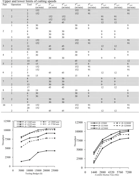
This paper demonstrates the importance of incorporating and solving the machining optimisation problem jointly with part selection and machine loading problems in order to avoid unbalanced workload in the FMS. Unbalanced workload renders to ineffective FMS such that some machines on the manufacturing shop floor become more occupied than others. Since CNC machine tools employed in the FMS are rather expensive, it is mostly important to balance the workload so that all machines can be effectively utilised. Therefore, in this study, two mathematical models are presented and solved in efforts to balance the workload and improve the performance of the FMS. A two-stage sequential approach is adopted whereby the first stage deals with the maximum throughput objective while the second stage deals with the minimum production cost objective. The results show that when part selection, machine loading and machining optimisation problems are jointly solved, more practical decisions can be made and a wide range of balanced workload in the FMS can be realised with minimum production cost objective. The results also show that the available machine time and tooling budget have enormous effects on throughput and production cost.
© 2011 Growing Science Ltd. All rights reserved
Keywords:
Part selection Machine loading Machining optimisation Flexible manufacturing systems
1. Introduction
Intensive market competition has forced manufacturing industries to focus on flexible manufacturing systems (FMSs). This is because FMSs offer a rapid and timely response to market demands thus helping the manufacturing industries to win competitive advantage. FMSs are highly automated manufacturing systems that consist of a group of processing workstations, usually computer-numerical control (CNC) machine tools, interconnected by automated material handling and storage systems altogether interfaced via a central computer. They are designed to combine the flexibility of a low-production-volume job shop and the efficiency of a high-production-volume flow shop to best suit the batch production of mid-volume and mid-variety of products. Job shop and flow shop are two conventional manufacturing systems that are associated with a traditional arrangement of machine tools on a manufacturing shop floor. In a job-shop system, machines are grouped together to perform similar operations for different parts. In a flow-shop system, machines are arranged together to process the parts as they flow from one machine to the next through the sequence of operations.
then effectively utilised to meet the production requirements, achieve the operational objectives and yet provide the payback more quickly. Various FMS planning problems have been addressed at different stages of the FMS’s life cycle. Stecke (1985) divided the FMS planning problems into five subproblems of part type selection, machine grouping, machine loading, production ratio, and resource allocation. Hwang (1986) found that among the five planning subproblems, part selection and machine loading are the most important in the FMS. However, the decisions of part selection and machine loading problems in the FMSs may not be effective because they often lead to unbalanced workload. As reported by Liang (1994), some planning policies such as maximising throughput may cause extremely unbalance workloads thereby causing bottleneck in some machines involved in the manufacturing process. The source for unbalanced workload decisions in part selection and machine loading problems may be the fact that the values of machining parameters are always predetermined and not optimised during FMS planning process as exhibited in Liang (1994), Yang and Wu (2002), and Choudhary, et al (2006).
The optimisation of machining parameters such as cutting speed, feed rate, and depth of cut is an essential step in achieving high machining efficiency and effective FMS. Ermer and Kromodihardjo (1981) and Manna and Salodkar (2008) optimised machining parameters for single machine problems while Agapiou (1992) optimised machining parameters for a conventional multi-stage machining system for effective machine utilisation. It is however learnt that previous studies on the optimisation of machining parameters mainly relied on either standalone machines or traditional multi-stage manufacturing systems rather than on FMSs. In order to utilise the machines in the FMS more effectively, it is necessary to determine the optimum machining parameters during the production planning stage. It is the purpose of this study to integrate the decisions of part selection, machine loading and machining optimisation problems in an attempt to balance the workload while improving the performance of the FMS.
2. Theoretical framework
2.1 Mathematical notations
The following mathematical notations are used for providing the theoretical concepts and in formulating the mathematical models for the FMS:
(1) Indices
j index for part type, j=1,..., J
k index for machines, k=1, …, K
o index for operations of part types, o,..., Oj
t index for tool type, t=1,..., T
(2) Decisions variables
xj = 1, if part type j is selected, 0 otherwise
xjotk = 1, if operation o of part j is processed using tool t on machine k, 0 otherwise
ytk = 1, if tool type t is assigned to machine k, 0 otherwise
vjotk cutting speed for combination j,o, t, k (m/min)
fjotk feed rate for combination j,o, t, k (mm/rev or mm/tooth)
pjk processing time of part j on machine k (min)
(3) Parameters
αjt tool life constant of the cutting speed for tool t on part j
γjt tool life constant of the depth of cut for tool t on part j
βjt tool life constant of the feed rate for tool t on part j
λjt tool life constant of the number of tool teeth in milling operations for tool t on part j
ωjt tool life constant of the tool diameter in milling operations for tool t on part j
δjt tool life constant of the width of cut in milling operations for tool t on part j
ajot depth of cut for operation o on part j using tool t (mm)
Ak available time at machine k (min)
B available tooling budget ($)
Ce tool cost of machining a single part ($)
Cm machining cost ($)
Cr tool replacement cost ($)
Ct cost per edge of tool t ($)
Djot tool diameter for operation o on part j (mm)
Ejt tool life constant for tool t on part j
FLjotk lower feed rate limit for combination j,o, t, k (mm/rev or mm/tooth)
FUjotk upper feed rate limit for combination j,o, t, k (mm/rev or mm/tooth)
Gk number of slots on tool magazine of machine k
Ljo length of cut for operation o on part j (mm)
Mjot, Njot machining constants for operation o on part j using tool t
Qj production quantity of part type j
qr number of parts per tool replacement
Rt replacement time for tool t (min)
St number of slots required by tool type t
Tjt tool life for part j and tool t combination
tm machining time (min)
tp processing time of a single part (min)
uj value coefficient of part j
VL
jotk lower cutting speed limit for combination j,o, t, k (m/min)
VUjotk upper cutting speed limit for combination j,o, t, k (m/min)
Wj width of cut on part j (mm)
Zt number of teeth of tool t
2.2 Theoretical concepts and main assumptions
The concept of solving part selection, machine loading and machining optimisation problems jointly comes with the need to define the relationship among their entities. In reality, processing time and tooling cost form a major linkage among part selection, machine loading and machining optimisation problems. On one hand, the selected parts for processing in the FMS depend on the available machine time. Similarly, due to higher tooling cost, the number of tools that can be loaded on the tool magazine depends on the available tooling budget. On the other hand, machining parameters, processing time and tooling cost are strongly coupled. For instance, at higher cutting speeds, machining time and the related cost are less but more cutting tools are consumed thus increasing tooling cost. Major components of processing time are machining time and tool replacement time.
Machining time is the actual time required to process a part on a machine described as (Narang and Fischer, 1993):
1 1 − −
= jot jotk jotk
m N v f
t (1)
where
1000
jo jot jot
L D
N =π , for drilling and tapping/reaming operations, and (2a)
t jo jot jot Z
L D N
1000
π
= for milling operations. (2b)
Machining cost is the product of machining time and operating cost rate. Denoting Uo as the
operating cost rate, the machining cost can be written as:
o jotk jotk jot
m N v f U
C = −1 −1 (3)
Tool replacement time is the time needed to remove a worn tool from the machine and replace with a new tool. Tooling cost is the cost of purchasing new cutting tools. Both the tool replacement time and tooling cost are functions of the Taylor’s tool life equation. The extended tool life equation reported by Lambert and Walvekar (1978) can be written in the following form:
jt jt jt
jot jotk jotk
jt jt
a f v
E
T = α β γ (4)
The tool life is reached and the tool can be replaced when several parts have been processed on a machine. It follows that the number of parts at each tool replacement is the ratio of tool life in Eq. (4) to unit machining time in Eq. (1) expressed as:
jt jt jt
jot jotk jotk jot
jt r
a f v N
E
q = α β γ (5)
Substituting Eqs. (2a) and (2b) into Eq. (5) and rearranging the terms, the tool replacement time and tooling cost distributed to each part can be respectively presented as:
t jotk jotk jot
r M v f R
t = αjt−1 βjt−1 (6)
and,
t jotk jotk jot
e M v f C
Mjot is a machining constant which is defined by Wang and Liang (2005) as: jt jo jot jot E L D M jt 1000
1−ω
π
= for drilling operations
(8a) and, jt jot jo jot jot E a L D M jt jt 1000
1−ω γ
π
= for reaming/tapping operations (8b)
The machining constant for milling operations defined by Shnumugam, et al (2002) and Wang and Liang (2005) is:
jt t j jot jo jot jot E Z W a L D M jt jt jt jt 1000 1 1−ω γ δ λ −
π
= (8c)
Correspondingly, the tool replacement cost is the product of tool replacement time and operating cost rate and is defined as:
o t jotk jotk jot
r M v f RU
C = αjt−1 βjt−1 (9)
Taking the sum of machining time in Eq. (1) and tool replacement time in Eq. (6), the processing time can be represented as:
t jotk jotk jot jotk jotk jot
p N v f M v f R
t = −1 −1 + αjt−1 βjt−1 (10)
In similar manner, adding up the machining cost in Eq. (3), tool cost in Eq. (7), and tool replacement cost in Eq. (9), the total production cost can be obtained as:
o t jotk jotk jot o jotk jotk jot
p N v f U M v f RU C = −1 −1 + αjt−1 βjt−1
t jotk jotk
jotv f C M αjt−1 βjt−1
+ (11)
As shown earlier, both processing time and tooling cost make a significant link among part selection, machine loading and machining optimisation problems. Therefore, Eq. (7), Eq. (10) and Eq. (11) are accordingly useful for the formulation of mathematical models in the subsequent sections. Before formulating the models, the main assumptions are defined as follows:
(1) The manufacturing parameters are deterministic and static. Breakdowns on machines are not considered and parameters are considered as constant and hence do not change over time. (2) The depths of cut of part-tool-machine combinations are known and given.
(3) The compatibilities of part-machine and tool-part combinations in the FMS are given.
(4) A part type is selected or rejected for processing before the beginning of the production period and remains unchanged during this period.
(5) The CNC machining centres are identical and can perform different operations on any part type. One machining centre can process one operation at a time.
(6) Machining, loading and unloading workstations have sufficient input and output buffer spaces. (7) Machining centres, raw materials, parts and tools are simultaneously available in the beginning
of the production period.
(8) The material handling system, pallets and fixtures are fully available.
(9) Setting-up of parts is performed offline and the times required for transferring parts between machining centres are negligible.
3. Methodology
minimised while making the decisions of machine loading and machining optimisation but retaining the maximum throughput obtained in the first stage. The two-stage sequential approach was chosen primarily to avoid the complexity of meeting two different objectives concurrently in one aggregate planning problem.
Computational experiments are designed for sensitivity analysis, which involves varying the values of some control factors and examining how the observed results change with variations in control factors. This would help to test out the range of validity of models and data, and also to get more insights of the results and consequently make easier to evaluate and interpret the results. A two-factor full factorial design was adopted with the available machine time and maximum tooling budget as control factors each assigned to 5 levels. Therefore, a total of 52=25 computational experiments were conducted using Extended LINGO 11 software.The two FMS models are formulated in the following subsections:
3.1 Maximisation of throughput
The primary objective in the first stage was to maximise the FMS throughput within the boundaries of the operational requirements. The decisions of the integrated part selection, machine loading (operation allocation, part routing and tool assignment) and machining optimisation (cutting speed and feed rate) problem can be obtained when the model is solved. The model for maximising the FMS throughput was formulated by Mgwatu, et al (2009) as follows:
max j j
J
j
ju x Q
∑
=1 (12) subject to j T t K k jotk x x =∑ ∑
=1 =1
, ∀(j, o) (13)
1
1 1 1 ≥
∑ ∑∑
= = = J j O o T t jotk jx , ∀k (14)
1 1 1 ≤
∑ ∑
= = j O o T t jotkx , ∀(j, k) (15)
tk J j O o jotk y x j ≤
∑ ∑
=1 =1
, ∀(t, k) (16)
k tk T
t
ty G S ≤
∑
=1
, ∀k (17)
(
N v f M v f R)
Qjxjotk Ak kJ j O o T t t jotk jotk jot jotk jotk jot j jt
jt ≤ ∀
+
∑ ∑ ∑
= = = − β − α − − ,1 1 1
1 1 1 1 (18) B y S Q C f v
M jotk jotk t j t tk J j O o T t K k
jot jt jt
j ≤ − β − α = = = =
∑ ∑ ∑ ∑
1 11 1 1 1
(19)
U jotk jotk L
jotk v V
V ≤ ≤ , ∀(j, o, t, k) (20)
U jotk jotk L
jotk f F
F ≤ ≤ , ∀(j, o, t, k) (21)
0
=
jotk
x or 1, ∀(j, o, t, k) (22)
0
=
j
x or 1, ∀j (23)
0
= tk
y or 1, ∀(t, k) (24)
j is selected, xj = 1, and 0 if otherwise. Constraint (13) states that the total proportion of a part
processed at all alternative machines using all feasible tools should be the same for all operations, either xjotk = 0 or 1. The variable xjotk = 1, if operation o of part j is processed using tool t on machine
k, and 0 if otherwise. To ensure that all machines are utilised in the shop floor, constraint (14) binds every machine to perform at least one operation on a part. Constraint (15) prevents recirculation of parts on machines and maintains the flexibility of the system. Constraint (16) ensures that if a part is allocated to a machine, the required tool ytk should be assigned to that machine. If tool type t is
assigned to machine k, ytk = 1, and 0 if otherwise. Constraint (17) restricts the total number tool types
needed on tool slots St not to exceed tool magazine capacity Gk. Constraint (18) forces the total
processing time at each machine not to exceed the available machine time Ak on the shop floor.
Constraint (19) assures that the total tooling cost is not beyond the available tooling budget B. Constraints (20) and (21) give the lower and upper bounds for cutting speed (VL
jotk, VUjotk) and feed
rate (FLjotk, FUjotk) respectively. Constraints (22) through (24) represent binary restrictions on the
decision variables.
3.2 Minimisation of production cost
The model in the second stage was formulated to minimise the production cost. The selected parts already obtained in the first phase were maintained and used among other input data in the second stage model. There was an attempt to re-assign the selected parts and reallocate the tools to machines, and also to re-optimise the cutting speed and feed rate for the purpose of exploring the most possible minimum production cost. Once the second stage model is solved, the decisions of machine loading (operation allocation, part routing, tool assignment), machining optimisation (cutting speed and feed rate), and processing times of parts on machines can be made. The formulation of the production cost minimisation model is presented as:
min
∑∑∑∑
(
)
∈ = = = − β − α − − + s j jt jt J j O o T t K k jotk j o t jotk jotk jot jotk jotk
jotv f M v f R U Q x N
1 1 1
1 1 1 1
∑∑∑∑
∈ = = = − β − α + s j jt jt J j O o T t K k tk t j t jotk jotkjotv f C Q S y M
1 1 1
1 1
, Js=
{
j|xj =1}
(25) subject to 1 1 1 =
∑ ∑
= = T t K k jotkx , j∈Js, ∀o (26)
1
1 1 ≥
∑∑∑
∈s = =
j J j O o T t jotk
x , ∀k (27)
1 1 1 ≤
∑ ∑
= = j O o T t jotkx , j∈Js, k (28)
tk J j O o jotk y x s j ≤
∑∑
∈ =1
, ∀(t, k) (29)
(
)
j jotkJ j O o T t t jotk jotk jot jotk jotk
jotv f M v f R Q x N s j jt jt
∑∑∑
∈ = = − β − α − − + 1 1 1 1 11 =h, ∀k (30)
k A
h≤ , ∀k (31)
(
)
j jotk jkO o T t t jotk jotk jot jotk jotk
jotv f M v f R Q x p N j jt jt = +
∑∑
= = − β − α − − 1 1 1 1 11 , j∈J
s, ∀k (32)
∑∑∑∑
∈ = = = − β − α ≤ s j jt jt J j O o T t K k tk t j t jotk jotkjotv f CQ S y B M
1 1 1
1
1 (33)
U jotk jotk L
jotk v V
U jotk jotk L
jotk f F
F ≤ ≤ , j∈Js, ∀(o, t, k) (35)
0
=
jotk
x or 1, j∈Js, ∀(o, t, k) (36)
Constraint (17), tk k T
t
ty G S ≤
∑
=1
, ∀k, and Constraint (24), ytk =0 or 1, ∀(t, k)
The objective function (25) minimises the production cost of the selected parts. Constraints (26)-(29) and Constraints (33)-(36) are equivalent to Constraints (13)-(16) and Constraints (19)-(22), respectively. Constraint (30) assigns equal processing time h at all machines to guarantee balanced workload in the FMS. In Constraint (31), the processing times at machines are bound within the available machine time. Constraint (32) specifies the processing time pjk of each part at different
machines.
4. Results and discussions
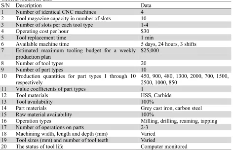
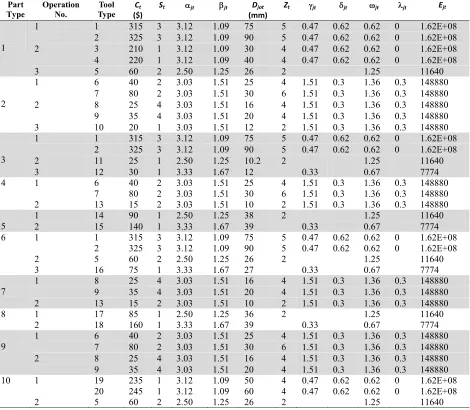
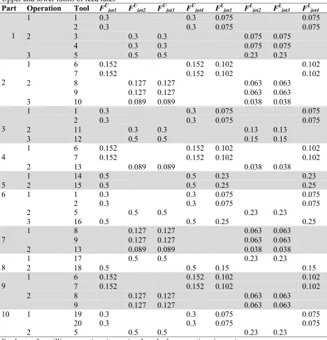
Both the formulated throughput and production cost models are integer nonlinear programming (INLP) problems and were computed using Extended LINGO 11 software. LINGO is a nonlinear programming software package which has the capability to solve nonlinear programming problems with unlimited number of linear and nonlinear constraints as well as unlimited number of integer, nonlinear and global variables (LINDO Systems Inc., 2008). The computations were conducted using the numerical data summarised in Table 1-Table 5. In the data, the tool-operation and tool-machine compatibilities are pre-specified. Tool life constants were taken from Shnumugam, et al (2002) and Wang and Liang (2005) while the tool costs per edge were obtained from McMaster-Carr Supply Company (2008). Limits of cutting speeds and feed rates were found in Chapman (2002).
Table 1
General industrial data
S/N Description Data
1 Number of identical CNC machines 4
2 Tool magazine capacity in number of slots 10 3 Number of slots per each tool type 1-4
4 Operating cost per hour $30
5 Tool replacement time 1 min
6 Available machine time 5 days, 24 hours, 3 shifts 7 Estimated maximum tooling budget for a weekly
production plan
$25,000
8 Number of tool types 20
9 Number of part types 10
10 Production quantities for part types 1 through 10
respectively 450, 900, 480, 1300, 2000, 700, 1500, 2500, 1000, 850 11 Value coefficients of part types 1
12 Tool materials HSS, Carbide
13 Tool availability 100%
14 Part materials Grey cast iron, carbon steel
15 Raw material availability 100%
16 Operation types Milling, drilling, reaming, tapping
17 Number of operations on parts 2-3
18 Machining width, length and depth (mm) Varied 19 Tool sizes (mm) and number of tool teeth Varied
Table 2
Tool and empirical data
Part
Type OperationNo. TypeTool ($)Ct
St
αjt βjt Djot
(mm)
Zt
γjt δjt ωjt λjt Ejt
1
1 1 315 3 3.12 1.09 75 5 0.47 0.62 0.62 0 1.62E+08
2 325 3 3.12 1.09 90 5 0.47 0.62 0.62 0 1.62E+08
2 3 210 1 3.12 1.09 30 4 0.47 0.62 0.62 0 1.62E+08
4 220 1 3.12 1.09 40 4 0.47 0.62 0.62 0 1.62E+08
3 5 60 2 2.50 1.25 26 2 1.25 11640
2
1 6 40 2 3.03 1.51 25 4 1.51 0.3 1.36 0.3 148880
7 80 2 3.03 1.51 30 6 1.51 0.3 1.36 0.3 148880
2 8 25 4 3.03 1.51 16 4 1.51 0.3 1.36 0.3 148880
9 35 4 3.03 1.51 20 4 1.51 0.3 1.36 0.3 148880
3 10 20 1 3.03 1.51 12 2 1.51 0.3 1.36 0.3 148880
3
1 1 315 3 3.12 1.09 75 5 0.47 0.62 0.62 0 1.62E+08
2 325 3 3.12 1.09 90 5 0.47 0.62 0.62 0 1.62E+08
2 11 25 1 2.50 1.25 10.2 2 1.25 11640
3 12 30 1 3.33 1.67 12 0.33 0.67 7774
4 1 6 40 2 3.03 1.51 25 4 1.51 0.3 1.36 0.3 148880
7 80 2 3.03 1.51 30 6 1.51 0.3 1.36 0.3 148880
2 13 15 2 3.03 1.51 10 2 1.51 0.3 1.36 0.3 148880
5 1 2 14 15 90 140 1 1 2.50 3.33 1.67 1.25 38 39 2 0.33 0.67 1.25 11640 7774
6 1 1 315 3 3.12 1.09 75 5 0.47 0.62 0.62 0 1.62E+08
2 325 3 3.12 1.09 90 5 0.47 0.62 0.62 0 1.62E+08
2 5 60 2 2.50 1.25 26 2 1.25 11640
3 16 75 1 3.33 1.67 27 0.33 0.67 7774
7 1 8 9 25 35 4 4 3.03 3.03 1.51 1.51 2016 44 1.511.51 0.30.3 1.36 1.36 0.3 0.3 148880 148880
2 13 15 2 3.03 1.51 10 2 1.51 0.3 1.36 0.3 148880
8 1 17 85 1 2.50 1.25 36 2 1.25 11640
2 18 160 1 3.33 1.67 39 0.33 0.67 7774
9 1 6 7 40 80 2 2 3.033.03 1.511.51 30 25 6 4 1.51 1.51 0.3 0.3 1.36 1.36 0.3 0.3 148880148880
2 8 25 4 3.03 1.51 16 4 1.51 0.3 1.36 0.3 148880
9 35 4 3.03 1.51 20 4 1.51 0.3 1.36 0.3 148880
10 1 19 235 1 3.12 1.09 50 4 0.47 0.62 0.62 0 1.62E+08
20 245 1 3.12 1.09 60 4 0.47 0.62 0.62 0 1.62E+08
2 5 60 2 2.50 1.25 26 2 1.25 11640
slots to be loaded as densely as possible. Therefore, the tooling cost and the penalty cost due to unused tool slots can be compromised basing on the economical benefits that suit the needs of a particular FMS.
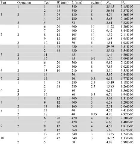
Table 3
Part and machining data
Part Operation Tool Wj(mm) Lj(mm) ajot(mm) Njot Mjot
1
1 1 68 540 5 25.45 3.15E-07
2 68 540 5 30.54 3.37E-07
2 3 26 180 8 4.24 6.36E-08
4 26 180 8 5.65 7.10E-08
3 5 32 2.61 3.82E-06
2
1 6 20 600 10 11.78 1.20E-04
7 20 600 10 9.42 8.44E-05
2 8 12 105 10 1.32 2.11E-05
9 12 105 10 1.65 1.95E-05
3 10 12 80 5 1.51 1.02E-05
3
1 1 68 630 4 29.69 3.31E-07
2 68 630 4 35.63 3.54E-07
2 11 45 1.44 6.80E-06
3 12 45 0.9 1.70 3.99E-05
4
1 6 20 500 8 9.82 7.12E-05
7 20 500 8 7.85 5.02E-05
2 13 10 210 6 3.30 3.55E-05
5 1 2 14 15 50 50 0.5 5.97 6.13 5.44E-06 6.77E-05
6
1 1 68 280 2.5 13.19 1.18E-07
2 68 280 2.5 15.83 1.26E-07
2 5 80 6.53 9.56E-06
3 16 80 0.5 6.79 6.94E-04
7
1 8 12 400 3 5.03 1.31E-05
9 12 400 3 6.28 1.20E-05
2 13 10 160 5 2.51 2.06E-05
8 1 17 40 4.52 4.41E-06
2 18 40 0.75 4.90 4.92E-05
9
1 6 20 420 4 8.25 2.10E-05
7 20 420 4 6.60 1.48E-05
2 8 12 360 4 4.52 1.81E-05
9 12 360 4 5.65 1.67E-05
10
1 19 42 340 3 13.35 1.24E-07
20 42 340 3 16.02 1.33E-07
2 5 50 4.08 5.98E-06
0 2500 5000 7500 10000 12500
0 5000 10000 15000 20000 25000
T
hr
ough
put
Tooling Budget ($)
A=1440 min A=2880 min A=4320 min A=5760 min A=7200 min
Table 4
Upper and lower limits of cutting speeds
Part Operation Tool VU
jot1
(m/min)
VU jot2
(m/min)
VU jot3
(m/min)
VU jot4
(m/min)
VL jot1
(m/min)
VL jot2
(m/min)
VL jot3
(m/min)
VL jot4
(m/min)
1
1 1 152 152 91 91
2 152 152 91 91
2 3 152 152 91 91
4 152 152 91 91
3 5 45 45 12 12
2
1 6 30 30 9 9
7 30 30 9 9
2 8 30 30 9 9
9 30 30 9 9
3 10 30 30 9 9
3
1 1 152 152 91 91
2 152 152 91 91
2 11 45 45 12 12
3 12 19 19 6 6
4
1 6 30 30 9 9
7 30 30 9 9
2 13 30 30 9 9
5
1 14 45 45 12 12
2 15 15 15 8 8
6
1 1 152 152 91 91
2 152 152 91 91
2 5 45 45 12 12
3 16 15 15 8 8
7 1 8 9 30 30 30 30 9 9 9 9
2 13 30 30 9 9
8
1 17 45 45 12 12
2 18 19 19 6 6
9
1 6 30 30 9 9
7 30 30 9 9
2 8 30 30 9 9
9 30 30 9 9
10 1 19 152 152 91 91
20 152 152 91 91
2 5 45 45 12 12
Fig. 1.Relationship between tooling budget and throughput Fig. 2. Relationship between available machine time and throughput 0
2500 5000 7500 10000 12500
0 1440 2880 4320 5760 7200
T
hr
oughput
Available Machine Time (Min)
Table 5
Upper and lower limits of feed rates
Part Operation Tool FU
jot1 FUjot2 FUjot3 FUjot4 FLjot1 FLjot2 FLjot3 FLjot4
1
1 1 0.3 0.3 0.075 0.075
2 0.3 0.3 0.075 0.075
2 3 0.3 0.3 0.075 0.075
4 0.3 0.3 0.075 0.075
3 5 0.5 0.5 0.23 0.23
2
1 6 0.152 0.152 0.102 0.102
7 0.152 0.152 0.102 0.102
2 8 0.127 0.127 0.063 0.063
9 0.127 0.127 0.063 0.063
3 10 0.089 0.089 0.038 0.038
3
1 1 0.3 0.3 0.075 0.075
2 0.3 0.3 0.075 0.075
2 11 0.3 0.3 0.13 0.13
3 12 0.5 0.5 0.15 0.15
4
1 6 0.152 0.152 0.102 0.102
7 0.152 0.152 0.102 0.102
2 13 0.089 0.089 0.038 0.038
5 1 2 14 15 0.5 0.5 0.5 0.5 0.23 0.25 0.23 0.25
6 1 1 0.3 0.3 0.075 0.075
2 0.3 0.3 0.075 0.075
2 5 0.5 0.5 0.23 0.23
3 16 0.5 0.5 0.25 0.25
7
1 8 0.127 0.127 0.063 0.063
9 0.127 0.127 0.063 0.063
2 13 0.089 0.089 0.038 0.038
8
1 17 0.5 0.5 0.23 0.23
2 18 0.5 0.5 0.15 0.15
9 1 6 7 0.152 0.152 0.152 0.152 0.102 0.102 0.102 0.102
2 8 0.127 0.127 0.063 0.063
9 0.127 0.127 0.063 0.063
10 1 19 0.3 0.3 0.075 0.075
20 0.3 0.3 0.075 0.075
2 5 0.5 0.5 0.23 0.23
Feed rates for milling operations in mm/tooth and other operations in mm/rev.
Table 6
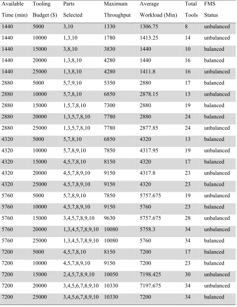
General results for maximum throughput model Available
Time (min)
Tooling
Budget ($)
Parts
Selected
Maximum
Throughput
Average
Workload (Min)
Total
Tools
FMS
Status
1440 5000 3,10 1330 1306.75 8 unbalanced
1440 10000 1,3,10 1780 1413.25 14 unbalanced
1440 15000 3,8,10 3830 1440 10 balanced
1440 20000 1,3,8,10 4280 1440 16 balanced
1440 25000 1,3,8,10 4280 1411.8 16 unbalanced
2880 5000 5,7,9,10 5350 2880 17 balanced
2880 10000 5,7,8,10 6850 2878.15 13 unbalanced
2880 15000 1,5,7,8,10 7300 2880 19 balanced
2880 20000 1,3,5,7,8,10 7780 2880 24 balanced
2880 25000 1,3,5,7,8,10 7780 2877.85 24 unbalanced
4320 5000 5,7,8,10 6850 4320 13 balanced
4320 10000 5,7,8,9,10 7850 4317.95 19 unbalanced
4320 15000 4,5,7,8,10 8150 4320 17 balanced
4320 20000 4,5,7,8,9,10 9150 4317.8 23 unbalanced
4320 25000 4,5,7,8,9,10 9150 4320 23 balanced
5760 5000 5,7,8,9,10 7850 5757.675 19 unbalanced
5760 10000 4,5,7,8,9,10 9150 5760 23 balanced
5760 15000 3,4,5,7,8,9,10 9630 5757.675 28 unbalanced
5760 20000 1,3,4,5,7,8,9,10 10080 5758.3 34 unbalanced
5760 25000 1,3,4,5,7,8,9,10 10080 5760 34 balanced
7200 5000 4,5,7,8,10 8150 7200 17 balanced
7200 10000 4,5,7,8,9,10 9150 7200 23 balanced
7200 15000 2,4,5,7,8,9,10 10050 7198.425 30 unbalanced
7200 20000 3,4,5,6,7,8,9,10 10330 7197.675 34 unbalanced
Table 7
Decisions of part selection, machine loading and machining optimisation for maximum throughput model
Available
Time (min) Tooling Budget ($) Part Operation Tool Machine Cutting Speed (m/min)
Feed Rate (mm/tool or (mm/rev)
Part routes
1440 5000
3 1 1 1 96.1 0.103 M1→M3→M2
2 11 3 28.6 0.131
3 12 2 6 0.150
10 1 19 4 103.7 0.076 M4→M3
2 5 3 12 0.230
4320 15000
4 1 6 1 28.2 0.133 M1→M2
2 13 2 30 0.089
5 1 14 1 41 0.326 M1→M4
2 15 4 12 0.500
7 1 8 2 28.6 0.098 M2→M3
2 13 3 30 0.089
8 1 17 3 12.1 0.500 M3→M4
2 18 4 13.6 0.500
10 1 20 4 112.3 0.296 M4→M3
2 5 3 12.1 0.278
7200 25000
3 1 1 1 91 0.300 M1→M2→M3
2 11 2 41.3 0.300
3 12 3 16.9 0.277
4 1 7 4 22.5 0.145 M4→M3
2 13 3 22.7 0.063
5 1 14 4 44 0.320 M4→M1
2 15 1 14.4 0.351
6 1 1 4 91 0.192 M4→M3→M1
2 5 3 21.8 0.365
3 16 1 8 0.311
7 1 8 3 30 0.073 M3→M2
2 13 2 29 0.069
8 1 17 2 31.7 0.366 M2→M4
2 18 4 9.5 0.486
9 1 7 1 29 0.127 M1→M2
2 8 2 19.7 0.063
10 1 19 1 91 0.265 M1→M2
2 5 2 12.1 0.233
machines and thus balancing the workload in the FMS. Other observations are that, in some cases, the average workload and tool slot usage decreased with time and tool cost savings as compared to those observed in the first stage.
Table 8
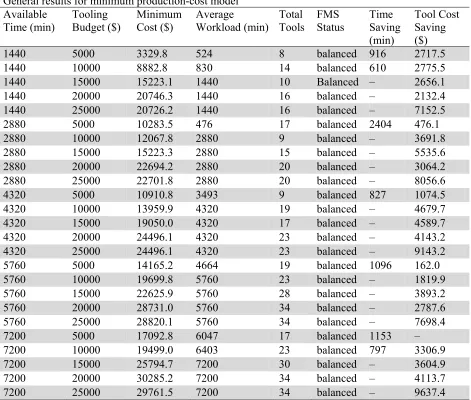
General results for minimum production-cost model Available
Time (min) Tooling Budget ($) Minimum Cost ($) Average Workload (min) Total Tools FMS Status Time Saving (min)
Tool Cost Saving ($)
1440 5000 3329.8 524 8 balanced 916 2717.5
1440 10000 8882.8 830 14 balanced 610 2775.5
1440 15000 15223.1 1440 10 Balanced – 2656.1
1440 20000 20746.3 1440 16 balanced – 2132.4
1440 25000 20726.2 1440 16 balanced – 7152.5
2880 5000 10283.5 476 17 balanced 2404 476.1
2880 10000 12067.8 2880 9 balanced – 3691.8
2880 15000 15223.3 2880 15 balanced – 5535.6
2880 20000 22694.2 2880 20 balanced – 3064.2
2880 25000 22701.8 2880 20 balanced – 8056.6
4320 5000 10910.8 3493 9 balanced 827 1074.5
4320 10000 13959.9 4320 19 balanced – 4679.7
4320 15000 19050.0 4320 17 balanced – 4589.7
4320 20000 24496.1 4320 23 balanced – 4143.2
4320 25000 24496.1 4320 23 balanced – 9143.2
5760 5000 14165.2 4664 19 balanced 1096 162.0
5760 10000 19699.8 5760 23 balanced – 1819.9
5760 15000 22625.9 5760 28 balanced – 3893.2
5760 20000 28731.0 5760 34 balanced – 2787.6
5760 25000 28820.1 5760 34 balanced – 7698.4
7200 5000 17092.8 6047 17 balanced 1153 –
7200 10000 19499.0 6403 23 balanced 797 3306.9
7200 15000 25794.7 7200 30 balanced – 3604.9
7200 20000 30285.2 7200 34 balanced – 4113.7
7200 25000 29761.5 7200 34 balanced – 9637.4
Fig. 3. Relationship between Tooling Budget and Production
Cost Fig. 4.
Relationship between available machine time and production cost
Table 9
Decisions of machine loading and machining optimisation for minimum production-cost model
Available
Time (min) Tooling Budget ($) Part Operation Tool Machine Cutting Speed
(m/min)
Feed
Rate (mm/tool or (mm/rev)
1440 5000
3 1 1 4 91 0.300
2 11 3 24.4 0.300
3 12 2 6 0.260
10 1 19 1 91 0.239
2 5 3 16.2 0.500
4320 15000
4 1 7 1 20 0.152
2 13 2 26.5 0.089
5 1 14 1 45 0.500
2 15 4 11.5 0.500
7 1 8 2 23.9 0.127
2 13 3 16.9 0.089
8 1 17 3 17.6 0.500
2 18 4 11.4 0.500
10 1 19 1 91 0.300
2 5 3 13 0.500
7200 25000
3 1 1 4 91 0.300
2 11 2 22.5 0.300
3 12 3 6 0.500
4 1 7 1 20 0.152
2 13 2 17.2 0.089
5 1 14 4 45 0.500
2 15 1 8 0.500
6 1 1 1 91 0.300
2 5 3 14.2 0.500
3 16 4 8 0.400
7 1 8 2 15.5 0.127
2 13 3 18.1 0.089
8 1 17 3 19.1 0.500
2 18 4 7.9 0.500
9 1 7 4 29 0.152
2 8 3 12.9 0.127
10 1 19 1 91 0.300
2 5 2 14.9 0.500
0 7000 14000 21000 28000 35000
-5000 5000 15000 25000
Pr
oduct
ion Cost
($
)
Tooling Budget ($)
A=1440 min A=2880 min A=4320 min A=5760 min A=7200 min
0 7000 14000 21000 28000 35000
0 1440 2880 4320 5760 7200
Pr
oduct
ion Cost
($
)
Available Machine Time (Min)
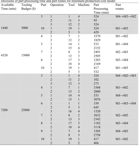
Table 10
Decisions of part processing time and part routes for minimum production-cost model Available
Time (min) Tooling Budget ($) Part Operation Tool Machine Part Processing Time (min)
Part routes
1440 5000
3 1 1 4 524 M4→M3→M2
2 11 3 95
3 12 2 524
10 1 19 1 524 M1→M3
2 5 3 429
4320 15000
4 1 7 1 3370 M1→M2
2 13 2 1829
5 1 14 1 533 M1→M4
2 15 4 2152
7 1 8 2 2491 M2→M3
2 13 3 2505
8 1 17 3 1283 M3→M4
2 18 4 2169
10 1 19 1 417 M1→M3
2 5 3 532
7200 25000
3 1 1 4 524 M4→M2→M3
2 11 2 102
3 12 3 273
4 1 7 1 3368 M1→M2
2 13 2 2800
5 1 14 4 533 M4→M1
2 15 1 3076
6 1 1 1 339 M1→M3→M4
2 5 3 645
3 16 4 1520
7 1 8 2 3832 M2→M3
2 13 3 2342
8 1 17 3 1182 M3→M4
2 18 4 3118
9 1 7 4 1505 M4→M3
2 8 3 2758
10 1 19 1 417 M1→M2
2 5 2 466
5. Conclusions
maximum throughput objective in the first stage. With minimised production cost, the bottleneck machines are eliminated and in some cases, the average workloads are decreased. This is a result of re-adjusting the machining parameters such as cutting speeds and feed rates, and also reallocating parts and reassigning tools on machines. The findings also support the applicability of the adopted approach over a wide range of planning period and tooling budget.
Acknowledgements
This research was supported by Sida-SAREC funding at the University of Dar es Salaam in Tanzania and Fulbright Scholarship for research visit at Lehigh University in United States of America.
References
Agapiou, J.S. (1992). Optimisation of multistage machining system, part 1: mathematical solution,
Journal of Engineering for Industry, 114(4), 524-531.
Chapman, W. (Ed.) (2002). Modern Machine Shop’s Handbook for the Metalworking Industries, Hanser Gardner Publications, 1st Edition, Cincinnati, Ohio, USA.
Choudhary, A. K., Tiwari, M.K., & Harding, J.A. (2006). Part selection and operation-machine assignment in a flexible manufacturing system environment: A genetic algorithm with chromosome differentiation-based methodology. Proceedings of the Institution of Mechanical
Engineers, Part B: Journal of Engineering Manufacture, 220(5), 677-694.
Ermer, D.S., & Kromodihardjo, S. (1981). Optimisation of multi-pass turning with constraints.
Journal of Engineering Industry, 103(3), 462-468.
Hwang, S. (1986). A constraint-directed method to solve the part selection problem in flexible manufacturing systems planning stage, Proceedings of the Second ORSA/TIMS Conference on
Flexible Manufacturing Systems, Ann Arbor, Michigan, USA, 297-309.
Lambert, B.K. & Walvekar, A.G. (1978). Optimisation of Multi-Pass Machining Operations.
International Journal of Production Research, 16(4), 259-265.
Liang, M. (1994). Integrating Machining Speed, Part Selection and Machine Loading Decisions in Flexible Manufacturing Systems. Computers in Industrial Engineering, 26(3), 599-608.
LINDO Systems Inc. (2008). LINDO User’s Guide, Chicago, Illinois, USA.
Manna, A., & Salodkar, S. (2008). Optimisation of Machining Conditions for Effective Turning of E0300 Alloy Steel. Journal of Materials Processing Technology, 203(1-3), 147-153.
McMaster-Carr Supply Company (2008). Cutting Tool E-Catalog, http://www.mcmaster.com, 1-3675, retrieved on Tuesday, 30th September 2008.
Mgwatu, M.I, Opiyo, E.Z. & Victor, M.A.M. (2009). Integrated Decision Model for Interrelated Sub-Problems of Part Design or Selection, Machine Loading and Machining Optimization, In Proceedings of the American Society of Mechanical Engineers (ASME) International Design
Engineering Technical Conferences and Computers and Information in Engineering Conference,
San Diego, California, USA, 3-12.
Narang, R.V. & Fischer, G.W. (1993). Development of a Framework to Automate Process Planning Functions and to Determine Machining Parameters. International Journal of Production Research, 31(8), 1921-1942.
Shnumugam, M.S., Reddy, S.V.B., & Narendran, T.T. (2002). Selection of Optimal Conditions in Multi-Pass Face-Milling Using a Genetic Algorithm, International Journal of Machine Tools and
Manufacture, 40, 401-414.
Stecke, K.E. (1985). Design, Planning, Scheduling, and Control Problems of Flexible Manufacturing Systems. Annals of Operations research, 3, 3-12.
Wang, P. and Liang, M. (2005). An Integrated Approach to Tolerance Synthesis, Process Selection and Machining Parameter Optimization Problems. International Journal of Production Research, 43(11), 2237-2262.