VOLUME 36, ARTICLE 35, PAGES 1015
−
1038
PUBLISHED 30 MARCH 2017
http://www.demographic-research.org/Volumes/Vol36/35/ DOI: 10.4054/DemRes.2017.36.35
Research Article
Examining the influence of major life events as
drivers of residential mobility and
neighbourhood transitions
Timothy Morris
© 2017 Timothy Morris.
This open-access work is published under the terms of the Creative Commons Attribution NonCommercial License 2.0 Germany, which permits use, reproduction & distribution in any medium for non-commercial purposes, provided the original author(s) and source are given credit.
1 Introduction 1016
1.1 Residential mobility 1016
1.2 Theoretical limitations within the literature 1017 1.3 Methodological limitations within the literature 1018
1.4 Study aim 1019
2 Methods 1019
2.1 Data 1019
2.2 Statistical analysis 1022
3 Results 1024
3.1 Descriptive statistics 1024
3.2 Recurrent events 1027
3.3 Unobserved confounding due to excluded life event data 1029
3.4 Stuck in place 1030
3.5 Competing risks 1031
4 Discussion 1032
5 Acknowledgements 1035
Examining the influence of major life events as drivers of residential
mobility and neighbourhood transitions
Timothy Morris1
Abstract
BACKGROUND
Residential mobility and internal migration have long been key foci of research across a range of disciplines. However, the analytical strategies adopted in many studies are unable to unpick the drivers of mobility in sufficient detail because of two issues prevalent within the literature: a lack of detailed information on the individual context of people’s lives and a failure to apply longitudinal methods.
OBJECTIVE/METHODS
Using detailed data from a UK birth cohort study, the Avon Longitudinal Study of Parents and Children (ALSPAC), and a multilevel recurrent-event history analysis approach, this paper overcomes these two major limitations and presents a number of findings.
RESULTS
Most life events increase the likelihood of moving, even though there is little evidence that they precede upwards or downwards mobility into more or less deprived neighbourhoods. The findings also suggest that families living in poor homes and neighbourhoods are more likely to be stuck in place following certain negative life events than those in good environments.
CONCLUSIONS
While broad demographic and socioeconomic characteristics reliably account for mobility patterns, the occurrence of life events and a person’s attitudes towards their living environment are necessary for a full understanding of mobility patterns. Future studies should strive to account for such detailed data.
CONTRIBUTION
We demonstrate the important impact that a wide range of life events has on the mobility of families and provide evidence that studies unable to account for major life events likely do not suffer strong bias results through unobserved confounding.
1. Introduction
1.1 Residential mobility
Residential mobility and internal migration have long been key foci of research across a range of disciplines, including demography (Champion 2005), health (Jelleyman and Spencer 2008), and education (Leckie 2009). This multidisciplinary interest has led to the extensive examination of mobility as both a cause and an outcome of various social processes. Traditionally, studies focussed on differences in broad social characteristics such as age and occupational social class between groups of mobile and nonmobile people, concluding that mobility patterns could largely be explained by such broad characteristics (Lee 1966; Bentham 1988). These findings led to the concept of selective migration – that individuals and families who move may differ from the populations in origin and destination areas and have differing capacities to select areas that they may migrate to compared to the general population. While this concept still underpins modern migration theory, in recent years there has been an increasing emphasis on how the specific context of people’s lives influences their mobility and migration patterns (Coulter and van Ham 2013). This approach argues that while broad social differences of mobile and nonmobile groups are important for determining group level patterns, it is individual, context-specific experiences that actively drive mobility by acting as exogenous shocks on people and their underlying mobility decision-making processes (Morris, Manley, and Sabel 2016).
This shift in focus complements recent advances in lifecourse theory within the mobility literature (Coulter, van Ham, and Findlay 2015). While a lifecourse approach is by no means new (Clark and Dieleman 1996), it has not yet been widely adopted. A lifecourse approach applied to mobility theorises that mobility behaviour cannot solely be explained by an individual or family’s status but also by important changes or life events that can occur throughout the whole lifecourse, from conception through to death (De Jong and Roempke Graefe 2008). This approach allows for drilling down into the heterogeneity of mobile and nonmobile groups and pulls away from notions of a simple ‘good/bad’ dichotomy that all people in these groups experience mobility in the same way. However, despite theoretical advances towards a lifecourse approach to mobility and calls for greater emphasis on the detailed context of individual lives, few studies have used data on individual life experiences such as major life events in a lifecourse framework when examining mobility (Morris, Manley, and Sabel 2016).
broad demographic and socioeconomic characteristics of mobile individuals, failing to account for life events or individuals’ attitudes towards the house and neighbourhood. Such missing key information risks unobserved confounding due to omitted variable bias in published findings. Secondly, the dominance of cross-sectional approaches throughout the literature makes it difficult to overcome issues of reverse confounding and to say anything about the temporal patterns of mobility, such as how life experiences at one point in time may influence mobility at another.
This paper uses longitudinal data and applies a lifecourse approach to investigate the impact that major family life events and attitudes towards the living environment have upon subsequent mobility. Data from the Avon Longitudinal Study of Parents and Children (ALSPAC), a UK birth cohort study, and an analytical approach is used to help overcome these two major limitations. I present evidence that shows that while broad demographic and socioeconomic characteristics are undoubtedly strong predictors of mobility, the occurrence of life events and opinions of the living environment are vital for a full understanding of mobility patterns. In this paper mobility is considered a microprocess focussing on the individual family unit, differentiated from migration as a macroprocess focussing on aggregated groups at the area level. However, the findings are also of relevance to macroprocess migration studies.
1.2 Theoretical limitations within the literature
While lifecourse theory in a mobility framework has advanced, empirical studies have been slow to adapt. A number of limitations persist which inhibit a full, contextualised understanding of mobility as a biographical event in the lifecourse (Morris, Manley, and Sabel 2016). There is a major theoretical limitation relating to the (lack of) important life event data used in many studies. While demographic and socioeconomic characteristics are often included in mobility studies, life events – the active drivers of mobility – are often excluded. Studies examining life events such as union formation (Grundy and Fox 1985) and dissolution (Flowerdew and Al-Hamad 2004; Feijten and van Ham 2007, 2010; Clark 2013), childbirth (Clark, Deurloo, and Dieleman 1994; Kulu 2005), and employment changes (Rabe and Taylor 2010) have determined that they exert an independent influence on increasing the likelihood of mobility over and above broad characteristics.
characteristics of mobile groups without life event data. These studies are important for understanding new cohort or population samples and cement the importance of broad characteristics in understanding mobility patterns. However, the inclusion of data on life events and opinions of the living environment in studies such as these would increase understanding of mobility in these cohorts as a process (although it is accepted that in numerous studies data limitations may prevent a more detailed analysis). Failing to account for such data limits our understanding of mobility.
Studies including life events have generally studied single events in isolation, meaning that it has been difficult to identify their relative importance. Some studies, however, have shed light on the way in which events can cooperate to influence mobility. Clark (2013) examined the impact of marriage, birth, separation, divorce, widowing, and job loss on mobility amongst an Australian sample and found that all events other than widowing were associated with an increased likelihood of making a residential move. Clark’s study was also one of very few to unpack divorce and separation into two separate events, finding that separation effects were twice as large as divorce effects (Clark 2013). Using UK samples, Coulter and Scott (2015) observed that marriage, separation, widowing, employment changes, and birth all increased the likelihood of mobility, while Rabe and Taylor (2010) found that childbirth and union dissolution both increased the likelihood of moving. Rabe and Taylor (2010) also accounted for neighbourhood opinions and observed that negative opinions were associated with increased mobility. De Groot and colleagues (2011) analysed multiple events alongside moving intentions in a Dutch sample and found that union formation and dissolution, child birth, and job change were all associated with increased mobility. They also went on to show that in each of these cases effects were stronger where people had no intention to move prior to an event occurring (de Groot et al. 2011), suggesting that unexpected shocks may disturb residential stability. These findings point to the importance of simultaneously considering multiple life events and opinions alongside broad characteristics when studying the drivers and patterns of mobility and migration.
1.3 Methodological limitations within the literature
cross-sectional framework. The use of such analyses may be born out of necessity due to cross-sectional data limitations, but where more detailed longitudinal data is available – as it widely is – such methods heavily limit the extent to which mobility can be understood. One methodological approach that is becoming more prevalent in mobility studies (De Jong and Roempke Graefe 2008; Ginsburg et al. 2011) and that is utilised here is an event history approach which focuses on the influence of both the occurrence and the timing of time-variant influences on mobility. This approach has not yet been used while considering life event data alongside broad characteristics in the context of studies examining mobility and migration.
1.4 Study aim
In this paper I argue that the omission of data on life events and subjective opinions of the living environment prevents a more detailed understanding of mobility patterns. I take a micro-perspective (at the family level) on the reasons that people move house and build upon previous work to make contributions to the literature in three areas: examining the role of a wider range of events than previously studied after accounting for demographic and socioeconomic characteristics, whether bias due to unobserved confounding may exist in broad characteristics where life events are excluded from analysis, and if life events influence subsequent mobility trajectories into more or less deprived areas. The dataset utilised in this study contains an extremely rich account of family life throughout time that is unique to population geography studies and allows for an examination of the drivers of mobility at a level of detail not possible in previous analyses of other datasets.
2. Methods
2.1 Data
The data comes from a UK longitudinal birth cohort study, the Avon Longitudinal Study of Parents and Children (ALSPAC).2 Pregnant women resident in the (former) Avon Health Authority area in South West England were eligible to enrol if they had an expected date of delivery between April 1991 and December 1992. For full details of the cohort profile and study design see Boyd and colleagues (2013) and Fraser and
2
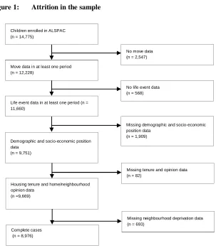
colleagues (2013). Data is utilised from mothers’ self-reports at seven time points from childbirth to child age 18. From the full enrolled sample of 14,775 children the analysis utilises data contributed by 8,976 mothers, resulting in 39,990 person-period observations (see Figure 1 for causes of attrition). The ALSPAC cohort is largely representative of the UK population when compared with 1991 census data; however, there is underrepresentation of ethnic minorities, single parent families, and those living in rented accommodation.
Figure 1: Attrition in the sample
Move data in at least one period (n = 12,228)
Life event data in at least one period (n = 11,660)
Missing demographic and socio-economic position data
(n = 1,909) No move data (n = 2,547)
No life event data (n = 568) Children enrolled in ALSPAC
(n = 14,775)
Demographic and socio-economic position data
(n = 9,751)
Missing tenure and opinion data (n = 82)
Housing tenure and home/neighbourhood opinion data
(n =9,669)
Complete cases (n = 8,976)
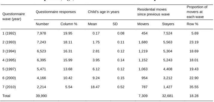
The outcome variable is any residential move as reported by the mother when their child was aged 2 months, and then at 2, 3, 4, 6, 9, and 18 years.3 Residential moves were coded 1 where a move occurred between the most recent and current questionnaire wave and 0 if no move occurred, providing a binary response variable indicating a move in the most recent period. Table 1 displays the responses and number of movers at each questionnaire wave used in the analysis.
Table 1: Responses, age, and residential moves at each questionnaire wave
Questionnaire wave (year)
Questionnaire responses Child’s age in years Residential moves since previous wave
Proportion of movers at each wave
Number Column % Mean SD Movers Stayers Row %
1 (1992) 7,978 19.95 0.17 0.08 454 7,524 5.69
2 (1993) 7,243 18.11 1.75 0.11 1,680 5,563 23.19
3 (1994) 6,523 16.31 2.81 0.12 1,219 5,304 18.69
4 (1995) 6,395 15.99 3.95 0.14 1,152 5,243 18.01
5 (1997) 5,471 13.68 6.12 0.12 1,063 4,408 19.43
6 (2000) 4,166 10.42 9.24 0.15 954 3,212 22.90
7 (2010) 2,214 5.54 18.47 0.52 787 1,427 35.55
Total 39,990 7,309 32,681 18.28
Note: SD: standard deviation. Year represents the year that questionnaires were sent to participants.
A range of life events are considered, including parental marriage, parental separation, parental divorce, parental job loss, death of a family member, illness of a family member, and sibling birth. Mothers were asked at regular intervals to report whether or not they had experienced each event.4 These were recorded for the same periods as residential moves, ensuring temporal consistency of data. Separation, divorce, and marriage are specified separately because a single marital status variable does not capture separation breaks in cohabitation, which are likely to be common given the proportion of nonmarried couples in the data. In addition to these life events, information was also collected on subjective opinions of the home and neighbourhood,
3
Mothers were asked about household moves by ALSPAC on additional occasions (8 months, 5 years, 11 years) but covariate data was not collected at all of these time points. For analysis purposes, where covariate data was not collected, move data was combined over two questionnaire waves to provide a temporally consistent measure indicating a move between the current and previous measurement occasion.
4
and this data was lagged to ensure that stated opinions referred to the houses and neighbourhoods that participants had moved away from.
Families’ demographic characteristics and socioeconomic position (SEP) were collected at regular intervals and were split into time-varying and time-invariant covariates. Time-varying covariates include financial difficulty,5 housing tenure, a variable indicating cumulative mobility throughout the study, and quintiles of neighbourhood deprivation measured by the UK Index of Multiple Deprivation (2004) based on 2001 lower layer super output areas. Time-invariant covariates utilised in the analysis were social class based on occupation, parental education, and parental age at birth.6
2.2 Statistical analysis
In order to make full use of the data in an appropriate modelling framework, an event history approach is employed (Steele 2005; Mills 2010). This longitudinal method allows for the examination of how explanatory variables such as life events impact subsequent residential mobility, while accounting for elapsed time through the inclusion of a baseline hazard rate (the probability of an event occurring at a given time). It is this focus on timing that separates event history analysis from standard regression models, an important consideration to mobility studies because of the nonuniform way that mobility and life events occur throughout the lifecourse. Because the questionnaire data used does not contain the exact timing of residential moves and life events, this analysis models time as discrete, with the outcome a discrete hazard rate.
Since residential moves can be made multiple times by a family, this analysis uses a multilevel recurrent-event history approach to incorporate multiple moves. Family-specific episodes (the time to a residential move being made) at level 1 are nested within families at level 2, so that a family that moves multiple times contributes multiple data records to the analysis. In this model families continue to contribute information after the first residential move, unlike in a single-event model, where they would be removed from analysis after the first move. The model assumes a binomial distribution and is defined with a complementary log-log link function, as follows:
5
Financial difficulty is chosen as the measure of household financial situation over income as it is more consistently measured in ALSPAC throughout time.
6
log 1 − ℎℎ = + + + +
~ (0, )
where the responseℎ is the hazard (likelihood of a residential move) in period for family , is the overall intercept in log odds for moving house when all else is constrained to zero,∑ captures each time interval dummy and represents the effect of elapsed time since the response (the baseline hazard function), represents a one-unit change in a time-varying covariate7 in episode of individual at time , and represents a one-unit change in a time-invariant covariate measured at baseline. Because recurrent events are experienced by the same families, it is likely that they will be correlated to a greater extent than two events drawn at random from the sample population. This may be due to unobserved characteristics that affect a family’s hazard of a move across all event episodes (for example, some mothers may form coresidential partnerships quicker than others because of unmeasured personality traits). To overcome this problem of unobserved heterogeneity, a normally distributed random effect is included at level 2 to control for unobserved time-invariant characteristics that influence mobility throughout the study period. This model allows the baseline intercept to vary between families by amount , but it still restricts the hazard form (duration and covariate effects) to be the same across families and allows for the estimation of the independent effect that each of the predictor variables has on mobility. This approach provides a number of advantages over a traditional single-level analysis. Firstly, it allows the pooling of all repeated episodes within families to maximise the data used. Secondly, it avoids breaking the independence assumption that would be broken in a single-level model. Thirdly, it also enables an examination of how exposure to previous mobility events has an effect on later mobility. In summary, the model facilitates the estimation of the relative effects that multiple life events have on recurrent residential moves.
Because we are also interested in whether life events have an impact on the likelihood that people may move towards more or less deprived neighbourhoods, the model can be further advanced to incorporate a competing-risks framework. A competing-risks model allows the examination of the impact of life events on mutually exclusive (i.e., competing) outcomes, in this case differential transitions to a more or less deprived neighbourhood than the neighbourhood of origin. The competing-risks
7
model consists of equations to estimate the risk of multiple independent outcomes compared to the risk of no outcome event, as follows:
log ℎ
( )
1 − ℎ( ) =
( )+ ( )+ ( ) ( )+ ( ) ( )+ = 1, … ,
~ (0, )
whereℎ( ) corresponds to the hazardℎ of outcome event at period for family . In this case, two events are modelled – one for a transition into a less deprived neighbourhood and another for a transition into a more deprived neighbourhood.
The analytical strategy for both the recurrent-event and competing-risk models consists of three stages. First, a series of single-event analyses are presented to determine the independent association between life events and mobility. Second, events are mutually adjusted for each other in order to examine their conditional association with mobility. Third, covariates are adjusted for to examine how the relationship between life events and mobility is explained by families’ underlying demographic and socioeconomic characteristics.
3. Results
3.1 Descriptive statistics
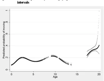
Figure 2: Predicted probability of moving by age of child with 95% confidence intervals
Note: Questionnaire data on moving was not collected between child ages 14 and 17.
neighbourhood were more likely to move than those who had positive opinions (p<0.001).
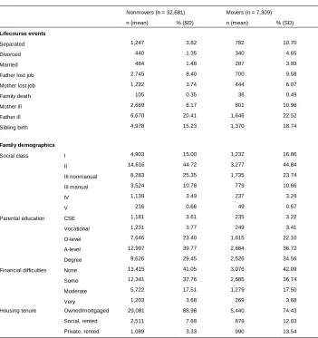
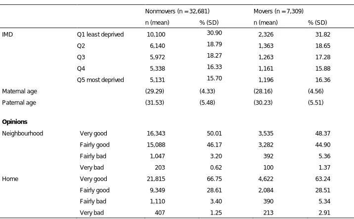
Table 2: Sample characteristics
Nonmovers (n = 32,681) Movers (n = 7,309)
n (mean) % (SD) n (mean) % (SD)
Lifecourse events
Separated 1,247 3.82 782 10.70
Divorced 440 1.35 340 4.65
Married 484 1.48 287 3.93
Father lost job 2,745 8.40 700 9.58
Mother lost job 1,222 3.74 444 6.07
Family death 105 0.35 36 0.49
Mother ill 2,669 8.17 801 10.96
Father ill 6,670 20.41 1,646 22.52
Sibling birth 4,978 15.23 1,370 18.74
Family demographics
Social class I 4,903 15.00 1,232 16.86
II 14,616 44.72 3,277 44.84
III nonmanual 8,283 25.35 1,735 23.74
III manual 3,524 10.78 779 10.66
IV 1,139 3.49 237 3.24
V 216 0.66 49 0.67
Parental education CSE 1,181 3.61 235 3.22
Vocational 1,231 3.77 249 3.41
O-level 7,646 23.40 1,615 22.10
A-level 12,997 39.77 2,684 36.72
Degree 9,626 29.45 2,526 34.56
Financial difficulties None 13,415 41.05 3,076 42.09
Some 12,341 37.76 2,685 36.74
Moderate 5,722 17.51 1,279 17.50
Very 1,203 3.68 269 3.68
Housing tenure Owned/mortgaged 29,081 88.98 5,440 74.43
Social, rented 2,511 7.68 879 12.03
Table 2: (Continued)
Note: SD, standard deviation; CSE, common certificate of education; IMD, index of multiple deprivation.
3.2 Recurrent events
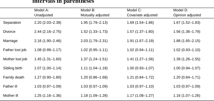
The main focus of the analysis is on the effects that the occurrence of major family life events have on the likelihood of making a residential move. Table 3 displays the results from the four event history analyses expressed as cluster-specific (family-specific) hazard ratios, showing the likelihood of moving house compared to remaining residentially stable given the occurrence of a life event within the period −1, . The assumptions for proportional hazards were satisfied for all variables with the exception of sibling birth and social class, which were modelled using interactions with elapsed time. These interactions ( < 0.001) indicated that delayed sibling birth was associated with a decreased likelihood of moving and that families in the lowest four social classes were disproportionately less likely to move as time passed than those in the highest two social classes.
Model 1 provides the unadjusted impact of each life event on the likelihood of making a residential move independently. Union formation and dissolution are the strongest predictors of a residential move – the occurrence of these events more than
Nonmovers (n = 32,681) Movers (n = 7,309)
n (mean) % (SD) n (mean) % (SD)
IMD Q1 least deprived 10,100 30.90 2,326 31.82
Q2 6,140 18.79 1,363 18.65
Q3 5,972 18.27 1,263 17.28
Q4 5,338 16.33 1,161 15.88
Q5 most deprived 5,131 15.70 1,196 16.36
Maternal age (29.29) (4.33) (28.16) (4.56)
Paternal age (31.53) (5.48) (30.23) (5.51)
Opinions
Neighbourhood Very good 16,343 50.01 3,535 48.37
Fairly good 15,088 46.17 3,282 44.90
Fairly bad 1,047 3.20 392 5.36
Very bad 203 0.62 100 1.37
Home Very good 21,815 66.75 4,622 63.24
Fairly good 9,349 28.61 2,084 28.51
Fairly bad 1,110 3.40 390 5.34
doubles an individual’s likelihood of making a residential move. Smaller effects are observed for sibling birth, maternal job loss, and maternal illness. Mutually adjusting life events (Model B) attenuates the impacts on mobility for all life event variables with the exception of sibling birth. The hazard ratio for parental divorce is heavily attenuated by the coadjusting effect of parental separation, indicating that the impact of divorce on moving may, to a considerable extent, be picking up the unmeasured effect of separation in the unadjusted model (I will return to this in the discussion). Adjusting for demographic and socioeconomic covariates (Model C) has an attenuating effect on most life events, but substantive conclusions remain the same for all events with the exception of sibling birth, which is attenuated to the null. Model D presents results from an analysis in which all life events are considered together alongside covariates and housing/neighbourhood attitudes. Adjustment for attitudes towards the home and neighbourhood has only a small attenuating effect on life events, and substantive conclusions from the models remain the same. A sensitivity analysis including lag and lead effects of life events on mobility demonstrated that the associations between life events and mobility were not biased by any potential anticipatory or delayed moves (Supplementary Table S3).
Table 3: Hazard ratios from event history analysis with 95% confidence intervals in parentheses
Model A: Unadjusted
Model B: Mutually adjusted
Model C: Covariate adjusted
Model D: Opinion adjusted
Separation 2.20 (2.03–2.38) 1.95 (1.79–2.13) 1.69 (1.54–1.86) 1.67 (1.52–1.83)
Divorce 2.44 (2.16–2.75) 1.52 (1.33–1.73) 1.57 (1.37–1.80) 1.56 (1.36–1.79)
Marriage 2.16 (1.90–2.46) 2.03 (1.79–2.31) 1.91 (1.67–2.19) 1.88 (1.65–2.15)
Father lost job 1.08 (0.99–1.17) 1.02 (0.95–1.11) 1.02 (0.94–1.11) 1.02 (0.93–1.10)
Mother lost job 1.45 (1.31–1.60) 1.37 (1.24–1.51) 1.41 (1.27–1.56) 1.39 (1.26–1.55)
Sibling birth 1.07 (1.00–1.14) 1.11 (1.04–1.18) 1.00 (0.93–1.07) 1.00 (0.94–1.07)
Family death 1.27 (0.90–1.80) 1.20 (0.86–1.68) 1.21 (0.84–1.72) 1.20 (0.84–1.71)
Father ill 1.03 (0.97–1.09) 1.03 (0.97–1.09) 1.03 (0.97–1.10) 1.03 (0.97–1.09)
Mother ill 1.25 (1.16–1.36) 1.18 (1.09–1.28) 1.17 (1.08–1.27) 1.16 (1.07–1.26)
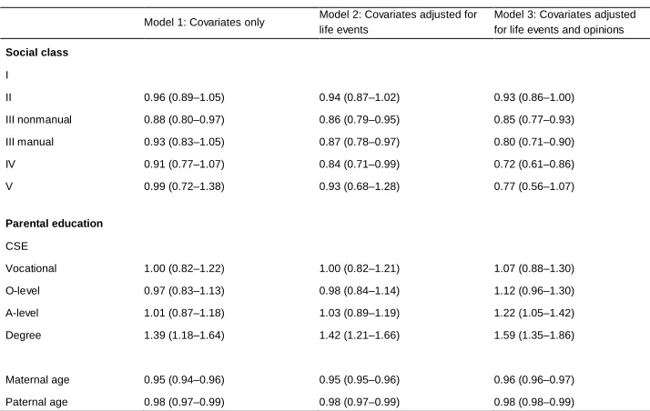
3.3 Unobserved confounding due to excluded life event data
Given the robust effects for numerous life events in Table 3, it is important to consider whether their exclusion leads to bias in results where only broad characteristics are considered. To test for the presence of such unobserved confounding, I conducted an analysis examining the change in hazard ratios of socioeconomic and demographic characteristics before and after adjusting for life events. The results of this analysis (see Table 4) demonstrate that excluding life event and opinion data results in an upward bias of estimates for social class and a downward bias for parental education. This is an important finding for the robustness of studies that only account for such characteristics, because it suggests that bias due to unobserved confounding is likely to be minimal.
Table 4: Bias due to unobserved confounding. Results expressed as hazard ratios with 95% confidence intervals in parentheses
Model 1: Covariates only Model 2: Covariates adjusted for life events
Model 3: Covariates adjusted for life events and opinions
Social class
I
II 0.96 (0.89–1.05) 0.94 (0.87–1.02) 0.93 (0.86–1.00)
III nonmanual 0.88 (0.80–0.97) 0.86 (0.79–0.95) 0.85 (0.77–0.93)
III manual 0.93 (0.83–1.05) 0.87 (0.78–0.97) 0.80 (0.71–0.90)
IV 0.91 (0.77–1.07) 0.84 (0.71–0.99) 0.72 (0.61–0.86)
V 0.99 (0.72–1.38) 0.93 (0.68–1.28) 0.77 (0.56–1.07)
Parental education
CSE
Vocational 1.00 (0.82–1.22) 1.00 (0.82–1.21) 1.07 (0.88–1.30)
O-level 0.97 (0.83–1.13) 0.98 (0.84–1.14) 1.12 (0.96–1.30)
A-level 1.01 (0.87–1.18) 1.03 (0.89–1.19) 1.22 (1.05–1.42)
Degree 1.39 (1.18–1.64) 1.42 (1.21–1.66) 1.59 (1.35–1.86)
Maternal age 0.95 (0.94–0.96) 0.95 (0.95–0.96) 0.96 (0.96–0.97)
Paternal age 0.98 (0.97–0.99) 0.98 (0.97–0.99) 0.98 (0.98–0.99)
3.4 Stuck in place
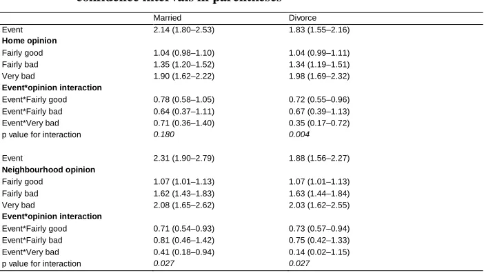
The analysis thus far concentrates on mobility but says little about residential immobility. While mobility theory suggests that families who experience life events are more likely to move, it is possible that major events may have the opposite effect on families that want to move and make them more likely to be stuck in place. To test if families who experienced life events but were living in subjectively poor houses and neighbourhoods were less likely to move than those who did not experience life events, a series of models with interactions specified between life events and home or neighbourhood opinions were run. Table 5 presents the results of these models for marriage and divorce, the only events for which interactions were detected. Families who had greater dissatisfaction with their environmental conditions and had experienced parental divorce were less likely to move than those who were dissatisfied but had not experienced divorce; that is, they were more likely to be stuck in place. A similar effect was observed for marriage, but only for neighbourhood satisfaction. These findings demonstrate the importance of considering residentially immobile families as a heterogeneous group.
Table 5: Interactions between marriage and divorce events and living environment opinions expressed as hazard ratios with 95% confidence intervals in parentheses
Married Divorce
Event 2.14 (1.80–2.53) 1.83 (1.55–2.16)
Home opinion
Fairly good 1.04 (0.98–1.10) 1.04 (0.99–1.11) Fairly bad 1.35 (1.20–1.52) 1.34 (1.19–1.51) Very bad 1.90 (1.62–2.22) 1.98 (1.69–2.32)
Event*opinion interaction
Event*Fairly good 0.78 (0.58–1.05) 0.72 (0.55–0.96) Event*Fairly bad 0.64 (0.37–1.11) 0.67 (0.39–1.13) Event*Very bad 0.71 (0.36–1.40) 0.35 (0.17–0.72)
p value for interaction 0.180 0.004
Event 2.31 (1.90–2.79) 1.88 (1.56–2.27)
Neighbourhood opinion
Fairly good 1.07 (1.01–1.13) 1.07 (1.01–1.13) Fairly bad 1.62 (1.43–1.83) 1.63 (1.44–1.84) Very bad 2.08 (1.65–2.62) 2.03 (1.62–2.55)
Event*opinion interaction
Event*Fairly good 0.71 (0.54–0.93) 0.73 (0.57–0.94) Event*Fairly bad 0.81 (0.46–1.42) 0.75 (0.42–1.33) Event*Very bad 0.41 (0.18–0.94) 0.14 (0.02–1.15)
p value for interaction 0.027 0.027
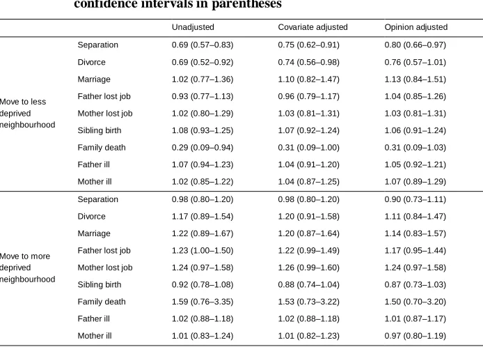
3.5 Competing risks
Table 6: Relative risk ratios from competing-risks analysis with 95% confidence intervals in parentheses
Unadjusted Covariate adjusted Opinion adjusted
Move to less deprived neighbourhood
Separation 0.69 (0.57–0.83) 0.75 (0.62–0.91) 0.80 (0.66–0.97)
Divorce 0.69 (0.52–0.92) 0.74 (0.56–0.98) 0.76 (0.57–1.01)
Marriage 1.02 (0.77–1.36) 1.10 (0.82–1.47) 1.13 (0.84–1.51)
Father lost job 0.93 (0.77–1.13) 0.96 (0.79–1.17) 1.04 (0.85–1.26)
Mother lost job 1.02 (0.80–1.29) 1.03 (0.81–1.31) 1.03 (0.81–1.31)
Sibling birth 1.08 (0.93–1.25) 1.07 (0.92–1.24) 1.06 (0.91–1.24)
Family death 0.29 (0.09–0.94) 0.31 (0.09–1.00) 0.31 (0.09–1.03)
Father ill 1.07 (0.94–1.23) 1.04 (0.91–1.20) 1.05 (0.92–1.21)
Mother ill 1.02 (0.85–1.22) 1.04 (0.87–1.25) 1.07 (0.89–1.29)
Move to more deprived neighbourhood
Separation 0.98 (0.80–1.20) 0.98 (0.80–1.20) 0.90 (0.73–1.11)
Divorce 1.17 (0.89–1.54) 1.20 (0.91–1.58) 1.11 (0.84–1.47)
Marriage 1.22 (0.89–1.67) 1.20 (0.87–1.64) 1.14 (0.83–1.57)
Father lost job 1.23 (1.00–1.50) 1.22 (0.99–1.49) 1.17 (0.95–1.44)
Mother lost job 1.24 (0.97–1.58) 1.26 (0.99–1.60) 1.24 (0.97–1.58)
Sibling birth 0.92 (0.78–1.08) 0.88 (0.74–1.04) 0.87 (0.73–1.03)
Family death 1.59 (0.76–3.35) 1.53 (0.73–3.22) 1.50 (0.70–3.20)
Father ill 1.02 (0.88–1.18) 1.02 (0.88–1.18) 1.01 (0.87–1.17)
Mother ill 1.01 (0.83–1.24) 1.01 (0.82–1.23) 0.97 (0.80–1.19)
Note: Events analysed independently of one another. Covariate coefficients suppressed; see Supplementary Tables S8–S16 for full model results.
4. Discussion
Additionally, it is important to consider not only mobile families, but also immobile families who may be stuck in undesirable home and neighbourhood environments following the occurrence of negative life events. Results from the competing-risks analysis suggest life events have little additional impact on the type of neighbourhoods that people move to, although the sample for this analysis was small and may have suffered from a lack of power to detect effects. Parental separation and divorce reduced the probability of families making a ‘positive’ move to a less deprived neighbourhood than to a neighbourhood with the same level of deprivation, while paternal job loss increased the probability of moving to a more deprived neighbourhood than to a similarly deprived neighbourhood. These results also suggest that movers may actually reinforce neighbourhood differences in deprivation through the transfer of unemployed individuals from less to more deprived areas, given that unemployment is one of the input variables for the IMD.
role in the mobility process above and beyond other factors, as has been suggested by others (Coulter and Scott 2015).
This study complements those that have used alternative methodological techniques to analyse the impact of life events on mobility. Clark’s study used a pooled cross-sectional approach and so was unable to measure longitudinal effects on the same individuals; Coulter and Scott used fixed-effects approaches and so were unable to include time-invariant characteristics; and De Groot and colleagues (2011) were only able to examine a short temporal snapshot of mobility. Like in Rabe and Taylor’s study (2010), the modelling approach used in this study accounts for time-stable unobserved differences between families. However, it is possible that these results may still be influenced by variant unobserved confounding, although the wide range of time-varying control variables that are utilised should minimise this. While each of these analytical techniques suffers limitations, they all do so differently, and the consistency in findings between this study and those referenced above provides robust evidence that life events and opinions of the living environment are important considerations for residential mobility, over and above broad socioeconomic and demographic characteristics.
recorded in the data. The fourth limitation relates to the measurement of deprivation used. Neighbourhood deprivation can vary over time, but by using deprivation data at only one time point, this study assumes deprivation to remain constant. While the use of multiple measures of deprivation at different time points throughout the study period was not possible due to comparability issues, there is evidence that deprivation levels remain relatively stable over time (Norman 2010) and, therefore, it is unlikely that the results are heavily biased. Future longitudinal studies may shed further light on the impact of place-specific changing deprivation and provide valuable insight to cohort studies and other data guardians in how to address these issues.
In conclusion, the results presented here suggest that life events are robust predictors of residential mobility. Studies should therefore account for the occurrence of life events and people’s attitudes toward the home and neighbourhood environment to permit a fuller understanding of residential mobility. Studies that are limited by data restrictions and do not account for such information are useful for describing populations and cohorts, but a more detailed examination of residential mobility as a biographical process, coupled with a lifecourse theory approach, is necessary for advancing our understanding of mobility and our ability to unpick the heterogeneity of mobile and immobile groups.
5. Acknowledgements
References
Bentham, G. (1988). Migration and morbidity: Implications for geographical studies of disease. Social Science and Medicine 26(1): 49–54. doi:10.1016/0277-9536(88)90044-5.
Boyd, A., Golding, J., Macleod, J., Lawlor, D.A., Fraser, A., Henderson, J., Molloy, L., Ness, A., Ring, S., and Davey Smith, G. (2013). Cohort profile: The ‘children of the 90s’ – The index offspring of the Avon Longitudinal Study of Parents and Children.Internatinal Journal of Epidemiology 42(1): 111–127.doi:10.1093/ije/ dys064.
Champion, T. (2005). Population movement within the UK. In: Chappell, R. (ed.).
Focus on people and migration. Basingstoke: Palgrave Macmillan: 91–113.
doi:10.1007/978-1-349-75096-2_6.
Clark, W.A.V. (2013). Life course events and residential change: Unpacking age effects on the probability of moving. Journal of Population Research 30(4): 319–334.
doi:10.1007/s12546-013-9116-y.
Clark, W.A.V. and Dieleman, F. (1996). Households and housing: Choice and outcomes in the housing market. New Jersey: Rutgers University, Center for Urban Policy Research.
Clark, W.A.V., Deurloo, M., and Dieleman, F. (1994). Tenure changes in the context of micro-level family and macro-level economic shifts. Urban Studies 31(1): 137– 154.doi:10.1080/00420989420080081.
Coulter, R. and van Ham, M. (2013). Following people through time: An analysis of individual residential mobility biographies. Housing Studies 28(7): 1037–1055.
doi:10.1080/02673037.2013.783903.
Coulter, R. and Scott, J. (2015). What motivates residential mobility? Re-examining self-reported reasons for desiring and making residential moves. Population, Space and Place 21(4): 354–371.doi:10.1002/psp.1863.
Coulter, R., van Ham, M., and Findlay, A.M. (2015). Re-thinking residential mobility: Linking lives through time and space. Progress in Human Geography 40(3): 352–374.doi:10.1177/0309132515575417.
Feijten, P. and van Ham, M. (2010). The impact of splitting up and divorce on housing careers in the UK. Housing Studies 25(4): 483–507. doi:10.1080/ 02673031003711477.
Flowerdew, R. and Al-Hamad, A. (2004). The relationship between marriage, divorce and migration in a British data set. Journal of Ethnic and Migration Studies
30(2): 339–351.doi:10.1080/1369183042000200731.
Fraser, A., Macdonald-Wallis, C., Tilling, K., Boyd, A., Golding, J., Davey Smith, G., Henderson, J., Macleod, J., Molloy, L., Ness, A., Ring, S., Nelson, S.M., and Lawlor, D.A. (2013). Cohort profile: The Avon Longitudinal Study of Parents and Children: ALSPAC mothers cohort. International Journal of Epidemiology
42(1): 97–110.doi:10.1093/ije/dys066.
Ginsburg, C., Steele, F., Richter, L.M., and Norris, S.A. (2011). Modelling residential mobility: Factors associated with the movement of children in Greater Johannesburg, South Africa. Population, Space and Place 17(5): 611–626.
doi:10.1002/psp.614.
De Groot, C., Mulder, C.H., Das, M., and Manting, D. (2011). Life events and the gap between intention to move and actual mobility. Environment and Planning A
43(1): 48–66.doi:10.1068/a4318.
Grundy, E. and Fox, A.J. (1985). Migration during early married life.European Journal of Population 1: 237–263.doi:10.1007/BF01796934.
Jelleyman, T. and Spencer, N. (2008). Residential mobility in childhood and health outcomes: A systematic review. Journal of Epidemiology and Community Health 62(7): 584–592.doi:10.1136/jech.2007.060103.
De Jong, G.F. and Roempke Graefe, D. (2008). Family life course transitions and the economic consequences of internal migration. Population, Space and Place
14(4): 267–282.doi:10.1002/psp.506.
Kulu, H. (2005). Migration and fertility: Competing hypotheses re-examined.European Journal of Population 21: 51–87.doi:10.1007/s10680-005-3581-8.
Lawrence, E., Root, E.D., and Mollborn, S. (2015). Residential mobility in early childhood: Household and neighborhood characteristics of movers and non-movers. Demographic Research 33(32): 939–950. doi:10.4054/DemRes. 2015.33.32.
the Royal Statistical Society: Series A (Statistics in Society) 172(3): 537–554.
doi:10.1111/j.1467-985X.2008.00577.x.
Lee, E.S. (1966). Theory of migration.Demography 3(1): 47–57.doi:10.2307/2060063.
Mills, M. (2010).Introducing survival and event history analysis. London: SAGE.
Morris, T., Manley, D., and Sabel, C.E. (2016). Residential mobility: Towards progress in mobility health research. Progress in Human Geography. doi:10.1177/ 0309132516649454.
Nivalainen, S. (2004). Determinants of family migration: Short moves vs. long moves.
Journal of Population Economics 17(1): 157–175. doi:10.1007/s00148-003-0131-8.
Norman, P. (2010). Identifying change over time in small area socio-economic deprivation. Applied Spatial Analysis and Policy 3(2–3): 107–138.doi:10.1007/ s12061-009-9036-6.
Rabe, B. and Taylor, M. (2010). Residential mobility, quality of neighbourhood and life course events. Journal of the Royal Statistical Society: Series A (Statistics in Society) 173(3): 531–555.doi:10.1111/j.1467-985X.2009.00626.x.
Steele, F. (2005). Event history analysis. Bristol: ESRC National Centre for Research Methods (NCRM methods review papers, NCRM/004). http://eprints.ncrm.ac.uk/88/1/MethodsReviewPaperNCRM-004.pdf
Thomas, M., Stillwell, J., and Gould, M. (2015). Modelling mover/stayer characteristics across the life course using a large commercial sample. Population, Space and Place 22(6): 584–598.doi:10.1002/psp.1943.