University of New Orleans University of New Orleans
ScholarWorks@UNO
ScholarWorks@UNO
University of New Orleans Theses and
Dissertations Dissertations and Theses
Spring 5-18-2018
Detecting Rip Currents from Images
Detecting Rip Currents from Images
Corey C. Maryan
University of New Orleans, [email protected]
Follow this and additional works at: https://scholarworks.uno.edu/td
Part of the Artificial Intelligence and Robotics Commons
Recommended Citation Recommended Citation
Maryan, Corey C., "Detecting Rip Currents from Images" (2018). University of New Orleans Theses and Dissertations. 2473.
https://scholarworks.uno.edu/td/2473
This Thesis is protected by copyright and/or related rights. It has been brought to you by ScholarWorks@UNO with permission from the rights-holder(s). You are free to use this Thesis in any way that is permitted by the copyright and related rights legislation that applies to your use. For other uses you need to obtain permission from the rights-holder(s) directly, unless additional rights are indicated by a Creative Commons license in the record and/or on the work itself.
Detecting Rip Currents from Images
A Thesis
Submitted to the Graduate Faculty of the University of New Orleans in partial fulfillment of the requirements for the degree of
Master of Science in
Computer Science
by
Corey Maryan
B.A. Southeastern Louisiana University, 2013
Acknowledgments
I would like to thank Dr. Mahdi Abdelguerfi for all of the opportunities he has given me
during my career at the University of New Orleans. He has given me more than I could ever ask
for. I would also like to thank him for recommending the thesis idea.
I would like to thank Dr. Md Tamjidul Hoque for providing me with the assistance I
needed for both the machine learning portion and writing portion of this project. He kept a
considerate attitude throughout the course of the project and was always eager to help.
I would also like to thank Dr. Elias Ioup and Dr. Christopher Michael for helping lay the
groundwork for collaboration with Naval Research Labs and for thesis guidance. I would also
like to thank Dr. Elias Ioup for jointly recommending the thesis idea.
Finally, I would like to thank Devin Frey for sparking my initial interest in computer
Table of Contents
Abstract ... vi
Introduction ...1
Literature Review...5
Machine Learning ...5
Neural Networks ...6
Support Vector Machines ...11
Ada-Boost ...15
PCA ...16
Other Machine Learning Algorithms ...17
Object Detection ...18
Haar Features ...24
Oceanography ...27
Orthorectification ...32
Methodology ...36
Rip Current Dataset...36
Max distance from the average ...37
Matlab ...37
Implementation ...38
Support Vector Machines ...38
Features for training ...38
Implementation ...39
Convolutional Neural Net ...40
TensorFlow framework ...40
Implementation ...41
Viola-Jones ...41
OpenCV library ...41
Implementation ...42
Meta Learner ...43
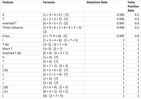
Additional Features ...43
Implementation ...45
Results ...48
Max distance from the average ...48
Support Vector Machines ...49
Convolutional Neural Net ...51
Viola-Jones ...52
Meta-Learner...55
New Features ...55
Stacking...56
Meta-learner ...57
Discussions ...61
Max distance from the average ...61
Support Vector Machines ...61
Convolutional Nueral Net ...62
Meta-Learner...64
New Features ...64
Classifier Stacking ...64
Conclusions ...66
Bibliography ...67
Appendices ...69
Ada-Boost in Java ...69
Integral Image in Java ...83
New Haar Features in Java ...86
Max distance from the average in Matlab ...92
Meta-Learner Feature Vector in Python ...98
Meta-Learner in Python ...104
List of Figures
Figure 1: Neural network node ...7
Figure 2: A Neural Network ...8
Figure 3: Neural network algorithm ...9
Figure 4: A hyperplane ...11
Figure 5: Non-linearly separability ...12
Figure 6: Maximal Margin ...13
Figure 7: Ada-Boost algorithm ...15
Figure 8: Attentional cascading ...18
Figure 9: The Viola-Jones Algorithm ...19
Figure 10: Viola-Jones image ...20
Figure 11: Example Haar Features ...24
Figure 12: Applying a feature ...25
Figure 13: Integral Image point ...25
Figure 14: Integral Image Regions ...26
Figure 15: A rip current ...27
Figure 16: Min max rip currents ...29
Figure 17: Transposed Sandbar locations ...31
Figure 18: Time averaged Shorline...32
Figure 19: Figure 18 transposed ...33
Figure 20: A picture from an Argus site ...34
Figure 21: Argus picture of rip currents ...34
Figure 22: Rain droplets...34
Figure 23: Sun blocking a camera ...34
Figure 24: Rip current samples ...36
Figure 25: Max distance from average ...37
Figure 26: TensorFlow Setup...40
Figure 27: Viola-Jones Model ...42
Figure 28: Matrix ...43
Figure 29: New Features results ...44
Figure 30: New Features ...45
Figure 31: Meta-classifier data ...46
Figure 32: Basic classifier parameters ...47
Figure 33: Meta-learner ...47
Figure 34: Max distance from the average ...48
Figure 35: Detection rate max distance ...49
Figure 36: False positive rate max distance ...50
Figure 37: SVM accuracy ...50
Figure 38: CNN detection rate ...51
Figure 39: CNN false positive count ...52
Figure 40: CNN image ...52
Figure 41: Viola-Jones Detection rate ...53
Figure 42: Viola-Jones False positive count ...54
Figure 43: Viola-Jones image ...54
Figure 45: Detection rate after stacking ...56
Figure 46: False positive rate after stacking ...57
Figure 47: Viola-Jones vs meta-learner detection rate ...58
Figure 48: Viola-Jones vs meta-learner false positive count ...58
Figure 49: Comparing detection rates ...59
Figure 50: Comparing false positive counts ...60
Figure 51: Viola-Jones vs meta-learner image ...60
Abstract
Rip current images are useful for assisting in climate studies but time consuming to manually
annotate by hand over thousands of images. Object detection is a possible solution for automatic
annotation because of its success and popularity in identifying regions of interest in images, such
as human faces. Similarly to faces, rip currents have distinct features that set them apart from
other areas of an image, such as more generic patterns of the surf zone. There are many distinct
methods of object detection applied in face detection research. In this thesis, the best fit for a rip
current object detector is found by comparing these methods. In addition, the methods are
improved with Haar features exclusively created for rip current images. The compared methods
include max distance from the average, support vector machines, convolutional neural networks,
the Viola-Jones object detector, and a meta-learner. The presented results are compared for
accuracy, false positive rate, and detection rate. Viola-Jones has the top base-line performance by
achieving a detection rate of 0.88 and identifying only 15 false positives in the test image set of
53 rip currents. The described meta-learner integrates the presented Haar features, which are
developed in accordance with the original Viola-Jones algorithm. Ada-Boost, a feature ranking
algorithm, shows that the newly presented Haar features extract more meaningful data from rip
current images than some of the current features. The meta-classifier improves upon the
stand-alone Viola-Jones when applying these features by reducing its false positives by 47% while
retaining a similar computational cost and detection rate.
1. Introduction
Rip currents are nearshore phenomena caused by the breaking of waves in an along-shore
direction. They account for the majority of lifeguard rescues at beaches. For oceanography, rip
current images assist in climate studies but must be manually annotated. “Argus site” locations
such as Duck, North Carolina hold rip current images in a backlog of beach imagery [1]. Argus
sites are groups of cameras that regularly take photos of shorelines. These images go through the
process of “orthorectification” [2],[3]. Othorectification alters the perspective of shoreline
photos by combining snapshots taken from cameras at different angles and turning them into one
image. The final image shows one, continuous bird’s eye view of the shoreline, which permits
easier identification of rip currents. There are many Argus sites at different locations taking
photos on an hourly basis. This amounts to several thousand images that may contain multiple
rip currents per image. Neither the time nor the manpower exist for manually annotating every
image, which makes conducting climate studies involving rip currents difficult. The lack of
resources creates a need for an automated method to find rip currents in images. The automation
of rip current detection can reduce the risk to swimmers and provide data for nearshore studies in
a shorter amount of time. Finding an efficient method to automatically find these rip currents
naturally lends itself to computing since computers process data far more quickly and accurately
than humans. Specifically, a branch of computer science called “machine learning” provides a
possible, effective solution because of its success in identifying regions of interest in images
[4-6].
Machine learning involves the development of algorithms that train models, which make
predictions on a set of test data [7]. Predicting the class of a data sample is known as
example, if a model trains to find rip currents in an image, then a collection of images is the test
data. Some images exemplify rip currents and have a class label of 1 while other images have a
class label of 0. The model is exposed to the images and trains with an algorithm. Then, the
model anticipates the class of unfamiliar images. Training a model with images involves
extracting data from each image via “computer vision” techniques. Computer vision is an area of
computer science concerned with image processing and “feature extraction” [8]. Feature
extraction collects descriptive data from each data sample, which trains a model. Feature
extraction, as a tool, reduces the amount of input data for the model. A large amount of data
yields more time and processing power for training. The reduction of input data makes feature
extraction important as it reduces runtime and conserves memory. A model identifies certain
areas in an image after it trains on computer vision features. Identifying a specific region of an
image with machine learning algorithms is “object detection”.
Object detection lends itself to a broad category than simply rip currents. Human faces
are a popular object for detection research [9],[10]. Models built for face detection train on
images of faces and develop from learning algorithms. An algorithm describes how a model
updates itself in accordance with the data. Learning algorithms find a pattern between samples
and update a model to achieve a higher performance on the dataset based on how many instances
a model incorrectly predicts. The most important goal for a detection model is finding an
accurate tradeoff between detected objects and misclassified non-object instances.
This thesis project aims to find a model that precisely detects rip currents from nearshore
imagery. Different methods for classification are compared, including: max distance from the
average [11], Support Vector Machines (SVM) [12], TensorFlow convolutional neural networks
Principle component analysis (PCA) [11] reduces the number of dimensions for a data
sample. This is important to the research as image data contain a large number of dimensions.
This project attempts to apply PCA to detection by finding the maximum distance from the
average data sample. A SVM [16] is another type of model that separates 2 classes with the
greatest distance by finding the maximal margin of separation. Classifier stacking [15] is a
meta-technique that trains a classifier on the output of many different models to increase accuracy.
TensorFlow is a framework developed by Google [13] and is applied to many machine
learning obstacles. Convolutional neural networks built with TensorFlow detect objects from
images. CNNs generate their own features through “image convolution” [4], [6]. Image
convolution applies a “kernel” to generate image effects, such as edge detection and blurs. A
kernel is a matrix paired with a region of an image and alters the makeup of the pixel it centers
around. These filters extract data from each image and eventually become features for training a
model. CNNs do not need their designs fine-tuned for a specific object when built with
TensorFlow [13], which makes them promising candidates for developing a rip current detection
model.
Another popular algorithm for object detection is “Viola-Jones” [10]. Viola-Jones
employs a unique set of features for extracting data, known as “Haar features”. Haar features are
sets of adjacent rectangles that correspond to different regions in an image. The value of a Haar
feature is extracted from the grey-scale pixel values in the rectangles. The values of Haar
features are generated while training the model. Viola-Jones has a technique to choose the best
Haar feature for the dataset [10]. The advantage of Viola-Jones is the speed of extracting Haar
The OpenCV package for Viola-Jones [14], TensorFlow framework [13] for CNN
models, Matlab for max distance from the average, and the Scikit-learn package [17] for basic
classifiers are run to generate results. Methods are a collection of machine learning tools, which
produces an object detection model in Python. Python is a popular programming language for
computer vision and machine learning because of the functionality already included. The built-in
implementation of the models are applied to the problem instead of constructing one from
scratch. Python is also user friendly and a viable choice for this project. Models make a
prediction on a dataset of rip current images and are compared with a predefined benchmark of
test images. The dataset is developed from 514 rip current samples manually extracted from the
surf zone of larger images. The large images are downloaded from a website of beach imagery
that contains many photos from previously mentioned Argus sites [1]. A larger dataset is created
by warping the samples from the smaller dataset with OpenCV.
This project expands upon the Haar feature space for the Viola-Jones classifier by finding
features better suited for rip currents. This project also contributes a meta-classifier that improves
upon the most accurate results of the current tools. The meta-classifier trains not only on the
output of many different models, but on the optimal Haar features chosen by the same algorithm
2. Literature Review
The literature review covers various topics relating to machine learning and how it is
involved with object detection and oceanography. The machine learning section covers different
algorithms applied in research. These algorithms are employed by object detection and can
extract data with Haar features. Certain oceanographic research involving rip currents depends
on these machine learning algorithms and orthorectification.
2.1 Machine Learning
Machine learning concerns fitting data to a model with an algorithm [12], [7]. The
models then make a prediction on a data sample with no class label. This prediction is conducted
with previous occurrences of similar data. For example, a model trains to predict whether a given
image is a rip current. The class of the image defines if it is a rip current. Images labeled 1 are of
rip currents or are labeled 0 if not of rip currents. The images in class 1 are positive samples
while the images in class 0 are negative samples. The learning algorithm processes training data
from each image. An example of training data is the location of dark regions in an image.
Machine learning implementations employ either “supervised”, “unsupervised”, semi-supervised
or reinforcement learning [7].
Unsupervised learning is the training of a model when the dataset has no class labels, or
“ground-truth” data [7]. The ground-truth data describes the correct prediction on a data sample.
Updating a model is more difficult when its predictions cannot compare with ground-truth data.
Unsupervised learning is applied when class labels are unknown. This can be useful for tasks
Supervised learning concerns a model trained with data that has class labels [7].
Supervised learning is the focus of this project because the location of rip currents in images is
known. The learning is supervised since the model’s predictions are compared to a class label.
These forms of learning are the training each model goes through.
Training data are a set of features, which describe each sample in a numerical fashion [7].
The evaluation of a model is performed after training. A model compares the predicted class to
the actual class. A “false negative” is an incorrect prediction on a positive sample. An incorrect
prediction on a negative sample is a “false positive”. A correct prediction on a positive sample
defines a “true positive”. A “true negative” identifies a correct prediction on a negative sample.
The goal of a model is to maximize the number of true positives while minimizing the number of
false positives. Maximizing true positives minimizes false negatives and minimizing false
positives maximizes true negatives. Learning algorithms such as neural networks, support vector
machines or Ada-boost enhance a model’s predictions on data.
2.1.1 Neural Networks
Neural networks form around the concept of the human brain [12]. Basic units in the
network are “nodes”. Nodes are similar to a neuron of the human brain. A node is made of three
parts, including: the input, the activation function, and the output. An example of a node is seen
in Figure 1. In Figure 1, the output of the neuron Y is equal to a function of its inputs. These
nodes connect to other nodes by links. The inputs of a node are outputs from other nodes. The
outputs result from multiplying each link weight by an input, then adding them together. Links
Links have a weight associated with them, which determine how strongly a node’s output is
considered when the network classifies a sample. The nodes become a network when every node
connects to every other node. An example network is in Figure 2. In Figure 2, a neural network
is made of three different layers: the input layer, the output layer, and a hidden layer. The input
layer takes the initial data. The output layer predicts the class label. The label is based on the
output from nodes in the hidden layers. A “single layer perceptron” is composed of an input
layer directly connected to an output layer [12]. A “multi-layer feed-forward network” has 1 or
more hidden layers. The hidden layers represent the complex relationships between the input and
output nodes. A more complex relationship needs additional hidden layers. The neural network
trains by propagating through these layers until it reaches the output layer. The network’s error is
the output found versus the desired output.
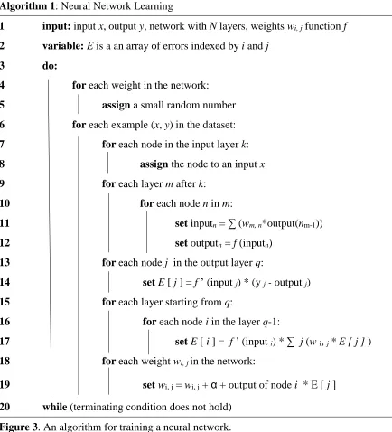
“Back-propagation” is the network updating the weights in reverse order [12]. The algorithm for
training a neural network is seen in Figure 3. In line 1 of Figure 3, the algorithm takes an input
dataset x and an output dataset y. A data structure is setup to store the error for each node.
Everything below line 3 repeats until convergence is determined at line 20. Small, random
numbers are assigned to every weight in the network. Each node in the input layer is then
assigned an input from the dataset. Line 9 starts forward propagation. The inputs and outputs for
every node of every layer after the input layer are calculated through the activation function. In
Line 13-14, the error of each node in the output layer is calculated in accordance with the class
label. Line 15-17 applies back-propagation. This starts from the output layer and works
backward. The error of each node is found until the input layer is reached. The weights update in
lines 18 and 19. In line 20 the network checks for convergence. The algorithm exits if the model
did not improve or ran a specific number of “epochs”. An epoch is an iteration of training for the
network. The algorithm resumes at line 4 if these conditions are not met.
Images contain vast information for a dataset. Building an efficient network is unrealistic
if the dataset is too large. For example, each pixel in a 224 by 244 image has 3 dimensions for its
red, green, and blue color value. A node is created for every pixel and every dimension
amounting to 150,528 nodes in the input layer. Parameters total to 22,658,678,784 after adding
the links to each node. The memory needs of parameters yield an inefficient use of resources. A
Algorithm 1: Neural Network Learning
1 input: input x, output y, network with N layers, weights wi, j function f
2 variable: E is a an array of errors indexed by i and j
3 do:
4 for each weight in the network:
5 assign a small random number
6 for each example (x, y) in the dataset:
7 for each node in the input layer k:
8 assign the node to an input x
9 for each layer m after k:
10 for each node n in m:
11 set inputn = ∑ (wm, n*output(nm-1))
12 set outputn = f (inputn)
13 for each node j in the output layer q:
14 set E [ j ] = f ’ (input j) * (y j - output j)
15 for each layer starting from q:
16 for each node i in the layer q-1:
17 set E [ i ] = f ’ (input i) * ∑ j (wi, j * E [ j ] )
18 for each weight wi, jin the network:
19 setwi, j = wi, j + α + output of node i * E [ j ]
20 while (terminating condition does not hold)
224 by 224 image is relatively small, which makes the creation of nodes more difficult for larger
images. Instead, a “convolutional neural network” is built.
A convolutional neural network uses image processing techniques to extract and learn
features [5]. The input from these features is sent to a traditional set of fully connected layers.
The extraction of features is performed through “image convolution”. Image convolution is the
application of a filter to an image. When performing convolution, a square matrix is placed over
some center point in the image (x, y). Each number in the matrix corresponds to a weight. An
output is generated by setting (x, y) equal to the result of multiplying the weights in the kernel
with the values at the positions around (x, y). The results are added together to produce (x, y)’.
Convolution transforms pixels, which finds edges or generates blur effects. The effect depends
upon the kernel. These operations are the basis for the “convolution layer”. The convolutional
layer is the first layer after the input layer in a convolutional neural network. The convolutional
layer contains a set hyperparmeters, including: the number of filters (kernels), the distance every
filter extends over the image (receptive field), the “stride”, and the amount of “zero-padding”.
Stride is the number of pixels skipped when centering the kernel at the next pixel in the region.
Zero-padding assigns values to regions outside the image, which handles cases when the kernel
falls out of bounds. The layer accepts an input region of the image and outputs a corresponding
volume of data based on the number of filters. For example, a region of input from an image is 7
by 7 by 3. The width, height, and depth of this volume are 7, 7, and 3 respectively. 2 kernels, 3
by 3 in size, are convoluted with the region. Convolution produces an output of size 3 by 3 by 2
if a stride of 2 is applied. The third dimension (depth) is equal to the number of filters given as
input. Local connectivity is an important property of the nodes in a convolutional layer. Nodes
dimension. The local connection heavily reduces the number of input parameters, which saves
memory. An activation layer applies an activation function to the input volume after a
convolutional layer. A recurrence of convolutional layers are each followed by an activation
layer, which is needed to transform the input for future layers. The data alters into input for the
fully connected layers as it passes through each convolutional layer since the number of input
dimensions gradually decreases. The convolutional layers intermingle with pooling layers.
The pooling layers reduce the size of the input volume on the width and height dimensions. This
reduction in volume assists the computational effort for convoluting at future layers. The data is
fed to a traditional feed- forward, fully-connected neural network for prediction on a class label.
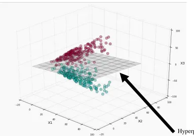
2.1.2 Support Vector Machines
Figure 4. An example of a hyperplane in a 3 dimensional space.
Another powerful learner is a support vector machine (SVM). A SVM finds the best
formula to separate data into different classes that have the greatest distance between them. This
is the “maximal margin” between classes and is represented by support vectors [12]. These
outlying points help form the boundary line between their class and a neighboring class, called a
“hyperplane”. An example is seen in Figure 4. In Figure 4, the hyperplane is the grid in grey
separating the two classes by intersecting the green points and red points. This example is
“linearly separable”. The relationships between non-linear input data and output data are not
separated into well-defined groups. The output is a set of points similar to Figure 5 if a graph is
shaped with non-linearly separable data. Notice the separating plane is not a function of the input
since the hyperplanes are curved in many directions. The most accurate hyperplane has the
largest margin of separation. “Margin” refers to the distance between the hyperplane and the
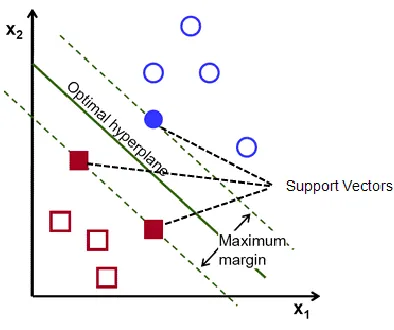
closest vector on each side of the plane. An example is seen in Figure 6. The solid colored
vectors in red and blue represent the support vectors and are closest to the separator.
Figure 5. An example of a non-linearly separability. The hyperplanes needed to separate the data are of complex shapes [16].
Non-linear hyperplane
Therefore, the margin is twice the distance from the separator to the closest support vector. Data
points are given a class, 1 or -1, in a binary classification problem. The separator is the set of
points defined by (1).
Finding this set of points involves solving the optimization problem defined in (2). New points
are classified by (3) after the optimum vector is found.
This solution works if the classes are linearly separable. “Data projection” is applied when
classes non-linearly separable and plots data in a higher or lower dimensional space. For
example, additional features are generated with (4), (5) and (6). Graphing in a 3-
Figure 6. A maximal margin. The margin is the distance of the closest support vectors in solid red and blue to one another. Each belong to a separate class. The optimal hyperplane is the center of the margin [18].
{𝑥 ∶ 𝑤 ∙ 𝑥 + 𝑏 = 0} (1)
𝑎𝑟𝑔𝑚𝑎𝑥 𝛼 ∑ 𝛼𝑗 − 1 2⁄ ∑ 𝛼𝑗𝛼𝑘𝑦𝑗𝑦𝑘(𝑥𝑗∙ 𝑥𝑘) (2)
dimensional space allows for more hyperplanes to be found because the data is now linearly
separable [12]. Projecting into higher dimensions is the “kernel trick”. The kernel function is
projecting the data and contains any number of dimensions. The dimensionality of the kernel
function allows for projection into a potentially infinite number of dimensions. A “hard margin”
is found when a margin separates data perfectly into each class by a straight line. Figure 6 is an
example of a hard margin. The separator is kept noisy when data is noisier. “Noise” is a property
of the data that distorts a data sample. An example is glare on a camera lens. A more realistic
classifier is produced if the separator retains the noisy property of the data. The target separator
is a “soft-margin” for non-linearly separable data. This margin adjusts itself for outlying points,
which increases the accuracy of the final classifier.
There are some disadvantages to SVM’s. SVM’s tend not to scale to a dataset that has
more dimensions than samples [7]. The correct kernel must also be chosen. A kernel to start with
is a “radial basis function” (RBF) kernel because it projects data into an infinite dimensional
space [7]. The input parameters “gamma” and “C” must also be chosen if the RBF is chosen. C
is the penalty parameter for incorrect classification and Gamma is the coefficient for the kernel.
These parameters are found through a process called “grid search”. Grid search tests a range of
gamma and C coefficients through “10-fold cross-validation”. 10-fold cross-validation breaks
data into 10 equally sized sets. The model trains on 9 folds and tests on the 1 remaining. The
model’s performance is a combination of testing results from each holdout fold after training on
the other 9. The best parameters are chosen based on the model’s performance.
𝑥12 (4)
𝑥22 (5)
𝑥1
1
2∙ 𝑥
2.1.3 Ada-Boost
Ada-boost searches through a set of features and ranks them in terms of error [19]. These
features build “decision stumps”, known as weak classifiers. Decision stumps are simple
classifiers that make a guess at classification, but are combined to form an
accurate model. Ada-Boost continuously re-evaluates a model with a test dataset and weighs
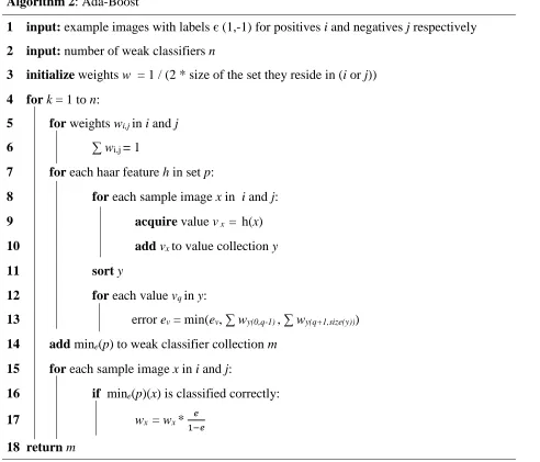
features accordingly. An example of the Ada-Boost algorithm is seen in Figure 7.
Algorithm 2: Ada-Boost
1 input: example images with labels є (1,-1) for positives i and negatives j respectively
2 input: number of weak classifiers n
3 initialize weights w = 1 / (2 * size of the set they reside in (i or j))
4 for k = 1 to n:
5 for weights wi,j in i and j
6 ∑ wi,j = 1
7 for each haar feature h in set p:
8 for each sample image x in i and j:
9 acquire value vx = h(x)
10 add vx to value collection y
11 sort y
12 for each value vq in y:
13 error ev = min(ev, ∑ wy(0,q-1) , ∑ wy(q+1,size(y)))
14 add mine(p) to weak classifier collection m
15 for each sample image x in i and j:
16 if mine(p)(x) is classified correctly:
17 wx = wx * 𝑒 1−𝑒
18 returnm
The inputs for Ada-Boost are a set of labeled images and the number of weak classifiers to
return. At line 3 the weights of each input image are initialized. Lines 5 through 17 repeat for
every weak classifier needed, which is based on n. Lines 5-6 normalize the weights of the images
every time a new search starts. Lines 7-13 repeat for every feature in the feature space. A feature
generates a collection of feature values after it is applied to the image collection. Lines 8-10
generate the feature values. Line 11 sorts the values and line 13 calculates the error for the
feature based upon the weights of the images. The error for the feature is found by comparing 2
different values. Errors are assigned at each feature value in the sorted set. The first error results
from setting all image above the current image to 1 and below to 0. The other error is found by
doing the opposite operation of the previous error. Error calculations are done in one pass over
the dataset. The feature with the minimum error is found at line 14, after every feature has an
error. The feature with the lowest error becomes a weak classifier. This weak classifier is added
to the current collection. In lines 15 through 17, the weight of the images update in reference to
images incorrectly classified by the weak classifier. The algorithm continues until k equals n.
An advantage of Ada-Boost is its resistance to “overfitting” the data [20]. Overfitting
occurs when the model learns the training dataset too well. This decreases generalization.
Generalization affects the prediction on samples not in the dataset. Ada-Boost also does not
require many parameters, which lowers memory needs [10].
2.1.4 PCA
Principle component analysis (PCA) is a method of analyzing the “variance” of a dataset.
Variance defines the difference between each data sample and the average data sample. PCA
reduces the number of dimensions in a feature vector [7]. Any dataset has a corresponding
the dataset. “Singular value decomposition” generates the Eigen vector by factoring the
covariance matrix [11]. The Eigen components are ranked from greatest to least variance
retained [11]. Dimension reduction employs Eigen components to project the dataset upon.
Projection is calculated through multiplication of the feature vector and the components, which
results in a new feature vector for the data sample. This vector has a size equal to the number of
components projected upon.
2.1.5 Other Machine Learning Algorithms
This section briefly outlines algorithms that create the meta-classifier. These algorithms
include: decision trees, K-nearest neighbors, Naïve Bayes and bagging.
A decision tree is a structure built from nodes and branches [21]. The branches extend
from every node. Nodes correspond to a test on an input variable while the branches are the
results of the test. Leaf nodes represent class labels when training a decision tree since they are
the final decision for the tree. Nodes check an input feature value, typically being for inequality
to a threshold value.
K-nearest neighbors (KNN) classify a data sample based on the class of a certain number
of neighbors, k [22]. Neighbors are assigned a weight based on how far they are from the sample.
Heftier neighbors have a greater impact on classification.
Naïve Bayes classifies a sample with the independent probability of features in the
training data [23]. The model assumes the probability of every feature is not dependent on the
probability of another feature, which drastically reduces the amount of computation needed to
train a classifier.
Bagging involves a variety of models that make a prediction on a data sample. Each
example, the outputs of a neural network, KNN, and Naïve Bayes are given a weight. A neural
network and Naïve Bayes model vote on the same class. The final output is their class since it is
2 to 1. However, the weight of KNN also affects the vote. If KNN has a larger weight than the
other two classifiers combined, then it chooses the class of KNN. The class predictions of these
algorithms assist in producing accurate object detection models.
2.2 Object Detection
Computer vision is the study of algorithms that alter and manipulate data contained in an
image [8]. The algorithms extract features for machine learning. Object detection is a
combination of computer vision and machine learning, which identifies certain regions of an
image. In contrast, object recognition concerns identifying a particular instance of an identified
object. Methods need “positive” and “negative” images. A positive image contains the object
being sought after while a negative image does not. Object detection also employs a training
algorithm, such as Viola-Jones or a convolutional neural network.
One type of object detection algorithm is the Jones object detector [10].
Viola-Jones uses Ada-Boost as the learning algorithm, Haar features, and “cascading architecture”. An
example of cascading architecture is shown in Figure 8. The detector starts with every sub
window in an image. Windows are checked at every position and scale in the image. Each sub
window is passed to a layer of the cascade for processing. The layers that vote the window
contains the object pass the image along to the next layer of the cascade. The layers that vote the
image does not contain the object discard it. The model is evaluated by its “detection rates” and
“false positive rates”. The detection rate is the number of positives correctly classified divided by
the total positive windows while the false positive rate is the number of negatives misclassified
divided by the total negative windows. A cascade’s detection rate and false positive rate are
equal to the product of every layers’ rate. For example, a cascading object detector has 4 layers.
Every layer has a detection rate of 0.99. The total detection rate for the classifier is 0.994 or 0.96.
Notice how the detection rate decreases as the number of layers increase. The detection rate
decreases because each layer cannot achieve a detection rate of 1.0, which causes them to lose
positive images. In contrast, the product of the false positive rates work in favor of the cascade.
Layers train to reject false positives of the previous layer. A higher detection rate and lower false
positive rate make it difficult to find a collection of suitable weak classifiers.
Only 0.067 seconds are needed to evaluate a 384 by 288 image on a 700 MHz Pentium
III processor [10]. The rapid detection speed creates “real-time object detection”. Real-time
object detection involves detecting objects at the speed of video frames and is associated with the
Algorithm 3: Viola-Jones Cascading Classifier
1 input: target false positive rate fp
2 input: false positive rate per layer fpi
3 input: detect rate per layer dti
4 input : set of positive and negative images j
5 variable i = 0 starting detection rate d = 1.0; starting false positive rate f = 1.0
6 whilef < fp:
7 i++
8 n = 0
9 while fpm< f * fpi-1
10 n++
11 collection of weak classifiers m = Ada-Boost(n,j)
12 evaluate collection on test set of images
13 while dtm < d * dti-1
14 decrease threshold k for collection and re-evaluate
15 setm as a layer i for cascaded classifier
16 delete any negatives in j correctly classified
rejection rate of negative samples. The rejection rate of negative samples depends on how low
the false positive rate per layer is set while the misclassification rate of positive samples depends
on how high the detection rate per layer is set. Negative windows are rejected quicker if the false
positive rate is lower. Positive images are more slowly discarded if the detection rate is higher.
An example of an image classified by the face detector is shown in Figure 9. The detected faces
are in red boxes.
An example of the Viola-Jones algorithm is seen in Figure 10. The Viola-Jones object
detector is given set of positive and negative examples on which to train and test. Other inputs
are an acceptable detection rate per layer, a target false positive rate, and a false positive rate per
layer. In line 5, i is initialized to 0. I represents the current layer the algorithm is building. The
starting false positive rate and detection rate for the cascade are initialized to 1.0. The classifier
considers every image a rip current when they are set to 1.0. Lines 6 through 16 repeat until the
classifier achieves the target false positive rate. At line 7 a new layer of the cascade starts. Line 8
sets the number of weak classifiers returned from Ada-Boost to 0. Line 9 through line 14 repeat
until the layer achieves the false positive rate needed. In line 10 the number of weak classifiers
needed increases. This starts at 1 to try the fastest possible computation time for each layer. At
line 11, Ada-Boost ranks every feature in the feature-space in terms of weighted error with the
algorithm described in section 2.1.3. Ada-Boost returns weak classifiers in a group of size n. The
collection becomes a potential layer of the cascade. On line 12 the algorithm evaluates the
performance of the layer by classifying a test set of images. Lines 13 and 14 repeat until the layer
has an acceptable detection rate. Decreasing the threshold causes the detection rate and false
positive rate. A layer with an acceptable false positive rate becomes a layer of the cascade.
Otherwise, the layer is discarded and the process starts over, with n increased by 1.
Open-source Computer Vision (OpenCV) is a Python package [14] for object detection
employing the Viola-Jones algorithm. The advantage the OpenCV implementation has over the
original is a more robust feature set [24]. This set includes features rotated at 45 degree angles.
OpenCV automatically produces a dataset by superimposing a slightly warped, positive sample
on top of negative sample. This introduces a risk of overfitting to an artificial dataset. The object
detector becomes adequate for only detecting artificial samples if the samples do not contain
meaningful data. The OpenCV package also saves a cascade by writing every layer to a file. The
files are accessed at a later time to continue training instead of building a new cascade from
scratch.
Recently, Google has implemented an object detection framework containing convolution
neural nets [9], called TensorFlow. This framework employs checkpoints of previous models,
which accelerates training to just a few hours [13]. Models built with TensorFlow spend weeks
training on many different objects. Then, they fine tune the final layer to the detect the object
needed [13]. TensorFlow has a variety of configurations for building a customized network. Two
examples are the Inception and Mobilenet models.
In [6], the authors address a need for an efficient convolutional neural network. The need
is generated from the current method for improving performance of a network, which involves
increasing the width and parameters of the network. This makes the network prone to overfitting.
The Inception model is introduced to alleviate the issue. 5 by 5 convolutions are expensive to
compute, given enough filters are applied at a convolution layer. A 1 by 1 convolution is applied
reduces the depth dimension. A 1 by 1 convolution keeps the same width and height of the input,
but reduces the depth if the number of filters applied is less than the previous output volume’s
depth. 1 by 1 convolutions make larger networks without sacrificing memory efficiency and
make local machines with less memory able to build larger networks. Inception networks consist
of inception modules, which contain a number of 1 by 1 convolution operations followed by a
larger size convolution or a pooling operation. The final Inception model has one fully-connected
layer at the end of the network. During training, it has a fully connected layer at the end of each
module in addition to a connection to the next module. This makes back-propagation start at
every module, which speeds up the training process. The fully-connected layers are discarded
after the model is complete.
Mobilenets are introduced in [4] as a different approach to reducing the size and
computational effort of convolutional neural networks. These networks contain “depth-wise
separable convolutions”. Depth-wise separable convolutions break up the convolution step into 2
parts. The first part involves applying a single filter to every input volume depth, called
“depth-wise convolution”. The second step applies a 1 by 1 convolution to the input volume. The 2
results are added together, which achieves a similar effect of normal convolution, but at a
reduced cost of parameters. The paper also introduces a method of thinning the network with a
“width multiplier”. This is a number less than one multiplied to the input depth and output depth.
The width multiplier reduces the width of each layer of the network, which further decreases the
cost of parameters.
Convolutional neural networks prove beneficial for building an object detector of many
different objects. Other approaches, like Viola-Jones, weigh heavily on the features they
2.3 Haar Features
Haar features form the main basis for a Viola-Jones [14] and are rectangular regions of an
image. The regions expose unique features extracted for training. Examples of Haar features are
seen in Figure 11. The feature (A) is known as “Four”, (B) as “Three Horizontal”, (C) as “Three
Vertical”, (D) as “Two Horizontal”, and (E) as “Two Vertical”. The feature types are chosen in
accordance with similarities of light and dark values in all faces [10]. The similarities are found
by taking a large set of face images, all of the same size, and averaging each pixel. An example
of an applied Haar feature is shown in Figure 12. The black regions of the Haar features are
covering the image with different orientations. The feature values are not calculated from the
original image, but from the “integral image”. An example is seen in Figure 13.
The value at (x, y) is the sum of the gray-scales values above and to the left of the pixel. The
difference between the areas under the rectangles is taken after the integral image values for each
of the rectangles are calculated. The difference of areas is the sum of integral image pixels in
white rectangles subtracted from the sum of pixels in black rectangles. An example of this is
shown in Figure 14. Figure 14 is a Haar rectangle with four regions: A, B, C, and D. The region
of A is the integral image value at point 1.
Figure 13. Integral Image point. The point (x, y) = sum of all pixels above and to the left of (x,
y).
Region B is the integral image value at point 2 subtracted from the value at point 1. Region C is
the integral image value at point 1 subtracted from point 3. Region D is the integral image value
at 4 added to the value at point 1. The final result is (1+4) – (2+3). Applying a Haar feature to an
image yields a single value, which is cheap to hold in memory and quickly computed. Integral
image values are accessed instantly while normal image values are iterated over. Therefore,
normal image values take more time to compute. The access speed results in immediate
evaluation time. A Haar feature placed at every width and height in a 24 by 24 image creates
over 160,000 features in the feature space. Ada-Boost iterates over the feature space every time a
weak classifier is needed. Adding more features slows down the search.
Normal Haar features are limited upright regions in horizontal and vertical directions.
The OpenCV implementation has a more robust set with rotated and upright regions [24]. The
original Haar features cannot locate tilted faces, which creates the need for rotated features.
These features are rotated by 45 degrees to mimic a rotated face.
There is no alternative to blunt force when searching for the optimal feature [25].
Searching the entire feature collection comprises the inefficiency of these features. Most
implementations of Viola-Jones have Haar features for face detection because they are optimized
for faces. There has been no further research into optimizing these features for different objects.
2.4 Oceanography
Oceanography is an Earth science coving a range of topics, including: ocean currents,
waves, plate tectonics and the sea floor [26]. Nearshore research comprises one area of
oceanographic research. An example of nearshore research are rip current studies. Rip currents
are narrow regions of the surf zone, are perpendicular to the shoreline, and are created by wave
breaking [28]. An example is shown in Figure 15 [27]. In Figure 15, the dotted line near the top
of the figure is a shoreline. The forces causing waves to move toward the shoreline are in purple.
The wave breaking forces are at opposite ends of the rip current and are in red and blue. More
than 100 people annually die from rip currents in the United States alone and rip currents account
for over 80% of the rescues performed by beach lifeguards [29]. People have a difficult time
recognizing rip currents when not trained to spot them [30]. Rip currents also play a large role in
beach erosion because of their seaward force from shoreline [31], which causes a large amount
of erosion for countries like Korea. Rip currents images assist in climate studies for
oceanography, but must be manually annotated by hand [32]. One image can contain many
different rip currents, which makes annotating thousands of images unreasonable. This can make
climate studies harder to conduct since they need the number of rip currents in each image and
the location of each rip current. The previous reasons generate the importance of an accurate
method for automatic rip current identification in images. One possible solution is machine
learning because it has become a popular, successful approach for locating certain regions of an
image [4-6].
Some oceanographic research is conducted with computer algorithms. One study
involves rip current behavior and video imagery [28]. In this study, a semi-automated algorithm
is introduced and adopts “local minima and maxima” for detecting rip channel patterns. The
local minima and maxima identify darkest and lightest areas of the image, respectively. The
algorithm is semi-automated because of human correction.Finding rip currents with light and
dark values is a contribution as the center of rip currents appear darker. A sample from the study
bottom of the image. In Figure 16, (a) the results of the automated portion of the algorithm are
shown.
Figure 16, (b) shows warmer colors for minima and cooler colors for maxima. Figure 16, (c)
shows the same shoreline after human modification. The algorithm finds the local maxima and
minima located in a 7.5 by 7.5 area of the image. All pixels outside the dotted area are not
considered since they are not near the shore. A few specification rules are introduced to
objectively remove pixels not considered part of the rip current. First, a rip current must be a part
of at least 5 connected local minima pixels. Second, segments of rip currents within 40 m of one
another are joined. Third, the rip current is split into 2 different rip currents if it has sections
connected by a line parallel to the shore. Finally, a rip current is removed if it does not extend
from the shoreline to the tip of the bar-line (dotted line). These images all have a similar
orientation, which allows the algorithm more generalizability. This makes the algorithm useful
for images distinct from the samples in the study.
Another study has already noted disadvantages of rip current imagery [33]. This study
discusses the “noise” found in such imagery. Noise makes it difficult to detect rip currents in
shoreline imagery because of how it interferes with meaningful data. An example could be rain
droplets or sun glare in the images. The solution is to apply a Gaussian blur, which filters out
noise. This involves a blending of color values of a particular group of pixels. Next, the image is
segmented into different regions based on the red, green, and blue values. Finally, color values
are grouped together to obtain a synthetic, noiseless image. A digitized version of rip currents are
manually created as a detection benchmark. This makes the process semi-automated. The
detection rate is 34% for original images and 41% for synthetic images. Correcting noise helps
minimize the variance of the samples, which generalizes the application of the algorithm.
In the following study, neural networks predict sandbar movement [34]. Sandbar
locations are output nodes and wave heights are input nodes. Predictions on sandbar locations are
more accurate when wave height is high and less accurate when the wave height is low. Previous
models cannot capture the data relationships because the data is non-linear. Hidden layers
capture non-linearity in data, which makes the study a contribution [7]. Example data from the
experiment is seen in Figure 17 [34]. The image in the top right is a bird’s-eye view and is
White, foamy regions from the image are placed onto a horizontal plane x (m). H (m) is wave
height over an 8 year period. Sandbar location is the data’s class label. In this situation, the
neural networks are “recurrent”. Ergo, the output of one time step is the input for the next time
step. For example, there is a sandbar location x (m)at time t. Wave height, averaged over time
t-1 through time t, predicts sandbar location at time t. Time step t becomes t-1 and predicts
sandbar location for the next time step t, previously t+1. A trained network predicts sandbar
locations outside of the training set.
Rip currents are a neglected focus of study for machine learning. The imagery from
previous studies has the potential for assisting in rip currents identification since it is
Figure 17. The white foam from the image in to top right is transposed onto x (m).
“normalized”. Normalization constrains data between 0 and 1, which highlights similarities in
extracted features. For images, this involves aligning each image to the same orientation and
size. These studies rely heavily on the bird’s-eye view images of the shoreline. These images are
not taken from a bird’s eye view, but created through the process of orthorectification.
2.5 Orthorectification
Previously mentioned studies [28],[34],[33] include imagery of rip currents. This is not
simple photography. Multiple cameras capture images of the shoreline at several different
angles. These images are “orthorectified”. This process converts the perspective of an image
into a different perspective [3],[2]. A 10 minute clip of video footage is averaged at every pixel
to enhance the wave and sandbar behavior in a resulting image. The image looks similar to
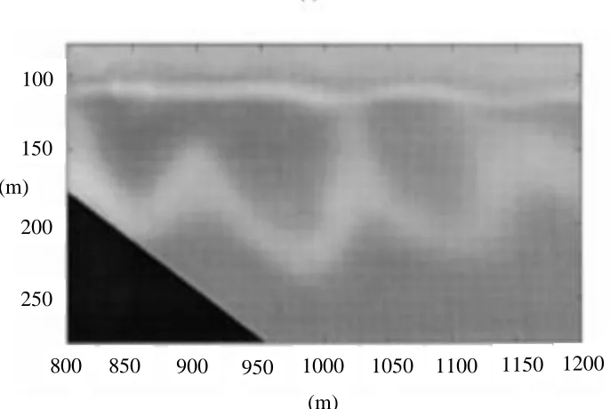
Figure 18 after it is averaged over 5-10 minutes [3].
In Figure 18, the surf zone of a beach front image is smoothed over time. The smoothing allows
the motion of the waves and sandbar location to appear well-defined. The center of the image is
used a reference point when transforming coordinates (x, y, z) into a 2 dimensional plane (u, v)
through matrix multiplication. The camera is calibrated after the multiplication is complete. The
camera is corrected through the equation described in [3],[2], hence the dotted region in the
image looks like Figure 19 [3]. Figures 18 and 19 are taken from an older Argus model from
1997. Argus sites [1], are set up at many beaches around the world. Multiple cameras are set up
for one beach. Combining the images at different locations produces a full view of the shoreline.
This is seen in Figure 20. Figure 20 is an example of an image from the Duck, North Carolina
camera site. In Figure 21, rip currents are darker blue regions of the surf zone, are surrounded in
red boxes, and are taken from Secret Harbour, Australia. Rip currents have less defined shapes
and sizes than other objects. There is some uncertainty whether the dark blue region farthest to
the right is a true rip current due to the horizontal orientation.
Figure 19. The dotted region of Figure 18 transposed onto a 2-D plane. 100
150
200
250
800 850 900 950 1000 1050 1100 1150 1200 (m)
Figure 20. An updated picture from an Argus site [1].
Figure 21. An Argus picture of rip currents.
Figure 22. An Argus picture with rain droplets on the lens of one camera.
Figure 23. An Argus picture with the sun blocking a camera.
Images can be distorted or unclear. An image looks like Figure 22 on a rainy day. In
Figure 22, rain is distorting one of the cameras. The rain produces a “stretched” look for the area
marked in red. In addition, Figure 23 is produced if the sun causes a reflection off of the ocean.
In Figure 23, lighter areas covering the shoreline are annotated in red. These distortions make
images not as desirable for a dataset. The images need to be as clear as possible to retain the
most meaningful data for a model. The orthorectified images create a usable dataset because of
their similar orientation for rip currents. A dataset of these images builds a rip current object
detector. Rip current regions in the images are pulled out of the larger image. The rip currents are
processed to create a list of descriptive features. The descriptive features train different models
for classifying images. There have been no studies applying machine learning to rip current
3. Methodology
The following topics describe the dataset and how it builds rip current object detectors.
Rip Current Dataset discusses how and where rip current images are generated from. These
images create training data and a benchmark for comparing different methods of rip current
classification. Next, the implementation and package details of max distance from average,
SVMs, convolutional neural network, Viola-Jones, and the meta-learner are shown. The new
features are revealed in the meta-learner section. The implementations explain how models
conduct classification. Methods generate a collection of values for comparison of detected rip
currents, including: accuracy, detection rate, false positive rate, and false positive count.
3.1 Rip Current Dataset
The data is downloaded from the Coastal Imaging lab web site [1]. The website contains
a collection of backlogged imagery from different beaches. An example is shown in Figure 24.
Figure 24 contains 5 rip currents extracted for training. These images are orthorectified by the
method mentioned in section 2.5. Orthorectification allows rip current images to have similar
orientation, which spawns similar features between the samples. All rip currents come
specifically from the Duck, North Carolina and Secret Harbour, Australia datasets. 514 examples
of rip currents, 24 by 24 in size, are extracted by hand from every image after shoreline images
are downloaded from the site. In addition, 800 24 by 24 negative examples are pulled in a similar
fashion from the surf zone. Surf zone negatives are part of the dataset because rip currents only
appear in images with a surf zone. Faces and other objects appear in many different places. The
false positive rate for the model reaches an acceptable level sooner when there are fewer types of
negatives to classify. Models created from negatives in any image are compared against surf
zone models.
3.2 Max Distance from Average
This section explains how to generate the max distance from the average rip current.
Then, the implementation of the classifier is described. This is the baseline classifier. Every other
classifier improves upon it.
3.2.1 Matlab
PCA runs on the set of rip currents, which finds the max distance from the average.
D. Only training on positive samples reduces the training data needed to create a classifier. This
eliminates computation effort as the size of the dataset has a significant impact on training time.
3.2.2 Implementation
A depiction of the implementation is seen in Figure 25. Every image is a 1 by 576 vector
when processed column wise. The 24 columns in the image are appended together to produce an
input vector. Singular value decomposition yields the Eigen vector for the collection of rip
current vectors. The vectors are projected toward the Eigen vector through matrix multiplication,
which creates a feature set for the image. The maximum distance from the average feature vector
is produced by finding the average feature vector. The resulting feature vector has size 1 when 1
component is projected toward. The average of the single values creates a midpoint in a range of
possible values. The absolute value of the greatest difference between any one sample feature
and the average is a threshold. This threshold classifies the images. Every component is
projected toward, which identifies the component with the smallest threshold. A projected
sample is classified as a rip current if it has a distance from the average less than or equal to the
threshold. It is classified as a non-rip current if the distance from the average is greater than the
threshold.
3.3 Support Vector Machines
This section reveals the SVMs built for classification. Formulas for processing the SVM
features and how the SVMs train on them are discussed.
3.3.1 Features for training
Meaningful features are the most important part in creating an accurate SVM [7]. Haar
a generous portion of image data. Not every feature is considered because the feature space is too
broad. SVMs do not scale well when there are more features than there are samples [7]. Instead,
an average of 10 Haar feature types are placed into the feature vector, which limits the training
vector size to 10 at the cost of descriptive information. This includes 5 new Haar identified in
section 3.7.1. Features in each category are grouped for averaging. The ratio of black to white
pixels in the image and “circularity” are also appended to the vector. Circularity represents how
close to a perfect circle an object is. An image consisting of either black or white pixels produces
a ratio between the two when they are counted and divided. A black and white image is
developed from setting every pixel in an image to totally black or totally white, which depends
on a threshold value. Circularity is calculated from a segmented image. A segmented image is
the result of applying a Matlab routine to a black and white image. Formula (7) produces
circularity. In the segmented image, bwow is the number of black pixels without a white
neighbor and bww is the number of black pixels with a white neighbor.
4𝜋(𝑏𝑤𝑜𝑤 𝑏𝑤𝑤⁄ 2) (7)
Circularity is a significant feature as rip currents have a semi-circular shape to them.
3.3.2 Implementation
The Scikit-learn package for Python creates and trains the SVM [17]. The SVM has a
RBF kernel because it projects data into an infinite dimensional space, which reveals
hyperplanes. 10-fold cross-validation evaluates the classifier. The model randomly chooses 10%
of the training data. The model tests on the 10% holdout after it finishes training on the other
only a few minutes to complete. A robust scaler from the Scikit-learn package scales the data
while grid search optimizes the results by finding C and gamma.
3.5 Convolutional Neural Networks
This section explains the CNNs compared. First, TensorFlow and the input needed to
train the networks are described. Next, how the networks intend to accomplish object detection is
revealed.
3.5.1 TensorFlow Framework
Tensorflow is a Machine Learning framework developed by Google. It is praised for its
fast training and ease of use [13]. TensorFlow supplies convolutional neural network
configurations for building models. Images generated from the OpenCV package train the
models. The training of convolution neural networks requires a large number of annotated
images. There are about 100 large, original images containing rip currents. More training
samples are needed. Therefore, they are trained on 4000 positive and 8000 negative images
generated by OpenCV. A record of every rip current location is created as input for the
framework. The models are evaluated on 10% of the training data.
3.5.2 Implementation
The convolutional neural network setup is seen in Figure 26. There are different model
configurations provided by Google [35]. One example is “SDD mobilenet V2 coco”. This model
trades training speed for accuracy. Another example is “faster rcnn inception resnet V2”.
Inception focuses on precision and accuracy in place of training speed as it has larger layers.
Training both models covers a wider range of CNN capabilities. Models are built from scratch
since the prebuilt models are not trained on rip current images [13]. The configurations for the
models are not changed from default. They run for 5 weeks and are evaluated on the same set of
orthorectified images as the other models.
The CNNs learn specific filters applied to different areas of an image. An example of a
filter is horizontal line detection. Thousands of samples teach CNNs important filters for a
specific object. Applying a certain filter activates a neuron path, which leads to a region
classified as an object of interest.
3.6 Viola-Jones
This section discusses the package containing an implementation of Viola-Jones. Then,
Viola-Jones is explained by showing how it classifies an image and showing the manner of
choosing its features.
3.6.1 OpenCV Library
OpenCV [14] is a popular python library that contains numerous methods to conduct
Machine Learning experiments. One built-in function trains a cascading object detector similar
to Viola-Jones [24]. OpenCV also has a method for automatically creating positive samples. The
![Figure 5. An example of a non-linearly separability. The hyperplanes needed to separate the data are of complex shapes [16]](https://thumb-us.123doks.com/thumbv2/123dok_us/8921365.1841799/20.612.112.535.91.300/figure-example-linearly-separability-hyperplanes-needed-separate-complex.webp)

![Figure 18 after it is averaged over 5-10 minutes [3].](https://thumb-us.123doks.com/thumbv2/123dok_us/8921365.1841799/40.612.153.466.392.660/figure-after-it-is-averaged-minutes.webp)