JIEM, 2014 – 7(4): 785-815 – Online ISSN: 2014-0953 – Print ISSN: 2014-8423 http://dx.doi.org/10.3926/jiem.1058
Integration of simulation and DEA to determine the most efficient
patient appointment scheduling model for a specific healthcare setting
Nazanin Aslani, Jun Zhang
North Dakota State University (United States)
[email protected], [email protected] Received: December 2013
Accepted: July 2014
Abstract:
Purpose:
This study is to develop a systematic approach for determining the most efficient
patient appointment scheduling (PAS) model for a specific healthcare setting with its
characteristics of multiple appointments requests in order to increase patients’ accessibility,
improve resource utilization, and reduce operation cost. In this study, three general
appointment scheduling models, centralized scheduling model (CSM), decentralized scheduling
model (DSM), and hybrid scheduling model (HSM), are considered.
Design/methodology/approach:
This study integrates discrete event simulation and data
envelopment analysis (DEA) to determine the most efficient PAS model. Simulation analysis is
used to obtain the outputs of different configurations of PAS, and the DEA based on the
simulation outputs is applied to select the best configuration in the presence of multiple and
contrary performance measures. The best PAS configuration provides an optimal balance
between patient satisfaction, schedulers’ utilization, and the cost of the scheduling system and
schedulers’ training.
in the interval from 15% to 25% the selected PAS model can be either DSM or HSM based on
expert idea. Similarly, if the proportion is in the interval from 50% to 70% the best PAS model
can be either CSM or HSM.
Originality/value:
This is the first study that determines the best PAS model for a particular
healthcare setting. The proposed approach can be used in a variety of healthcare settings.
Keywords:
data envelopment analysis, discrete event simulation, patient appointment scheduling,
multiple appointments, centralized scheduling model, decentralized scheduling model, hybrid
scheduling model
1. Introduction
Many outpatient clinics are facing the high pressure of reducing the cost and increasing the patient satisfaction. Patient appointment scheduling (PAS) has a significant impact on the clinic’s operation. An efficient PAS model is critical to achieving high accessibility, high resource utilization, and low cost (Gupta & Denton, 2008; Hooten & US ARMY Academy of Health Science, 1990).
Scheduling appointments in outpatient clinics is the process of assigning clinics’ timeslots to incoming requests (Guo, Wagner & West, 2004). Patients obtain appointments through a PAS system, which operates, based on the scheduling model. There are three major types of scheduling models: centralize scheduling model (CSM), decentralized scheduling model (DSM), and hybrid scheduling model (HSM). The performance of the PAS system is impacted by the interaction of the scheduling model used and the characteristics of the healthcare setting. The characteristics of the healthcare setting include a set of the attributes in each clinic, such as the arrival rate of demand and the percentage of patients with multiple appointments. If the PAS model is designed by not considering the characteristics of the healthcare setting, the PAS system would operate inefficiently (Nealon & Moreno, 2003). An efficient PAS system has the ability to provide a balance between the three indicators: cost, accessibility, and resource utilization.
The methodology used in this study is the integration of simulation and Data Envelopment Analysis (DEA) approaches to select the most efficient PAS model for a specific healthcare setting, as well as analyze the inefficient scheduling models, and identify parameters that may be altered to improve the overall system efficiency. Since it is not practical to apply different PAS models in the same healthcare setting to evaluate their performances due to the high interruption cost, this study applies simulation approach to obtain performance measures of different PAS models’ configurations that are needed for DEA outputs. Then DEA is applied to compare different scheduling models and select the most efficient scheduling model. Comparing the efficiency of scheduling models that have different attributes is a hard task. However DEA is a perfect tool which has the ability to compare the efficiency (or productivity) across different configurations (Avikran, 2001).According to our knowledge, this is the first research in the domain of healthcare operations that provides a generic framework to integrate simulation and DEA to find the most efficient PAS model for a specific clinic setting.
The structure of this study is as follow: Section 2 presents a literature review for the PAS system and DEA. Section 3 describes the problem statement as well as the framework structure to determine an efficient PAS model for a specific clinic setting. Section 4 presents the proposed methodology. Section 5 provides empirical examples in three different clinic settings to validate the usability of the proposed procedure. Finally, the conclusions for the study and other useful methodology that can be integrated with DEA in future research (for evaluating the efficiency of PAS model) are proposed in Section 6.
2. Literature Review
There are three major PAS models in terms of assigning timeslot(s) to the requested single or multiple appointments: CSM, DSM, and HSM (Zhang, Dharmadhikari & Song, 2009).
In CSM, a patient obtains appointments for multiple clinics or single clinic through one request, such as a phone call. Any scheduler can schedule appointments for all the clinics. The schedulers can locate in one central scheduling department or locate in different clinics or locations. In DSM, schedulers can only schedule patient appointments for one predefined clinic. If a patient has to request for multiple appointments, he or she will make multiple phone calls to obtain all the appointments. HSM is the combination of DSM and CSM. In HSM, some clinics operate under CSM and the rest of the clinics operate under DSM (Zhang, Gonela & Aslani, 2011; Berry & Phanthasomchit, 2000).
in how appointments are handled and better ability to monitor the entire process. The disadvantages of CSM are the needs for advanced information system and high skilled schedulers.
The advantages of DSM are: 1) the available capacity of the specific clinic is used efficiently, since the schedulers are familiar with the clinic resource; and 2) schedulers can schedule the clinic with the lowest cost. Implementation of DSM is useful in settings with a small number of clinics (Zhang, Gonela & Aslani, 2010; Zhang, Gonela & Aslani, 2011).However, if the number of patients with multiple appointments increases, the DSM might cause higher communication cost and conflicts among different clinics.
HSM takes the advantages of CSM and DSM. There is no need to have advanced information system and high skill level schedulers in HSM. When high interaction level requires between clinics and there is unavailability of advanced scheduling software, HSM is selected instead of CSM (Zhang, Gonela, & Aslani, 2010; Zhang, Gonela, & Aslani, 2011).The disadvantages of HSM are: sometimes it is required to contact more than one scheduler to schedule some of patients with multiple appointments due to the communication gap between the clinics with CSM and the clinics with DSM.
An inefficient PAS model would impose either high cost or lower patient dissatisfaction under certain healthcare settings. For example, if the healthcare setting is involved high volume of patients with multiple appointments and the PAS model is DSM, patients have to make multiple phone calls to schedule all the appointments. This will cause longer waiting time for the patients to get their appointments (each phone call might cause waiting time) and possible conflicts for the appointments.
In each PAS model (e.g., CSM), there are many configurations. Determining the most efficient appointment scheduling model between different generated configurations is complicated from general point of view. Firstly, different configurations cannot be easily compared because each configuration has its own attributes. Secondly, the objective function includes contrary performance measures. As a result, DEA is selected as the methodology to compare different configurations and select the most efficient configuration as well as analyzing the inefficient configurations.
at the operational level and suitable to use in studying healthcare systems (Peng, Niu & ElMekkawy, 2013; Jacobson, Hall & Swisher, 2013). Therefore, this study uses DES to obtain outputs of different configurations of PAS models.
DEA is an approach for evaluating the relative efficiency of either different organizations or different units in one organization. DEA has the capability of discriminating between multiple efficient units or organizations and determining the most efficient unit or organization (Yang & Kuo, 2003; Avikran, 2001). Additionally, DEA considers multiple inputs and outputs at the same time in the presence of complex relationships between inputs and outputs. This makes it different from several other efficiency approaches.
There are some studies in manufacturing industry which use DEA as a decision tool to select the most efficient staff allocation, staff training, and technology selection, such as the study for optimal operator allocation in cellular manufacturing (Ertay & Ruan, 2005).
There are some studies in healthcare area that integrate simulation and DEA to find out the most relative efficient system. Weng, Tsai, Wang, Chang and Gotcher (2011) apply the integration of DEA and simulation to find out the most relative efficient combination of nurses and physicians in emergency department through considering the utilization of nurses and physicians as well as patient waiting time as the performance measures. Al-Refaie, Fouad, Li and Shurrab (2014) apply the integration of simulation and DEA in the emergency department to find out the best distribution of nurses in order to increase utilization and decrease patient waiting time.
According to our knowledge, there are no studies in healthcare domain that apply analytical methods to determine the PAS model with the best allocation of schedulers, training level of schedulers, and complexity level of scheduling systems. In order to bridge the gap, this study proposes a method that integrates simulation and DEA to determine the most efficient PAS model for different healthcare settings.
3. Problem Statement
In order to increase patients’ accessibility, resource utilization, and reduce cost in hospitals or other healthcare settings, a framework is proposed to determine the most efficient patient PAS system for a specific healthcare setting with multiple appointments requests. Multiple appointments requests are considered as one of the major problems in appointment scheduling models (Nealon & Moreno, 2003).
defined as the ratio of patients requesting multiple appointments to the total patients requesting appointments. This index is used to classify healthcare settings.
Efficiency is evaluated through three categories of indicators relevant to PAS systems:
• Satisfaction indicator for patients, staffs, and managers
• Resource utilization indictor for schedulers
• Cost indicator for both complexity level of scheduling software and skill level of schedulers
One or multiple factors will be assigned to each category of indicators for evaluating the efficiency. Accessibility is defined as a factor for patient satisfaction. In this study, accessibility is measured by average waiting time before connecting to a scheduler and average call duration. The utilization of scheduler and the number of schedulers are the factors for resource utilization indicator. Complexity level of scheduling software and skill level of schedulers are the factors to cost indicator.
A framework is proposed to integrate simulation and DEA to determine the most efficient PAS model for a specific healthcare setting. The proposed methodology compares different configurations of different PAS models based on the three categories of efficiency indicators.
4. Proposed Methodology
First, different configurations based on the major PAS models (CSM, DSM, and HSM) are generated. Then, simulation models are built to obtain the outputs for the DEA model. The simulation outputs for the DEA model are staffs’ average utilization, patients’ average waiting time, and holding time in the system. Finally, the DEA model is implemented to determine the most efficient configuration from the generated configurations, and the reasons of inefficiency of other configurations.
The DEA inputs are the cost of scheduling software, the training cost, and the number of schedulers. The two cost-based inputs are obtained from the hospital administrator and vendors, and the number of schedulers is obtained from the queuing theory formula for the subjective service level (Agnihotri & Taylor, 1991).
schedulers with different skill level, the service level and the required number of the schedulers for different configuration.
The percentage of multiple appointments is obtained from the available historical data in the database. The clinics’ interaction index is the ratio of total number of multiple appointments over total number of appointments.
If the interaction index is less than 15 percent, the interaction level in the setting is low. If the interaction index is from 25 percent to 50 percent, the interaction level in the setting is medium. Finally, if the interaction index is more than 70 percent the interaction level in the setting is high. The interval from 15 percent to 25 percent is the threshold interval and the setting can be considered as either low or medium interaction level. In addition, the interval from 50 percent to 70 percent is the threshold interval and the setting can be considered as either medium or high interaction level.
4.1. Configuration generation
Different configurations for the three major PAS models (CSM, DSM, and HSM) are generated to provide sufficient number of alternatives. Sufficient number of alternatives should be evaluated to identify the best configuration of PAS model for a healthcare setting.
4.1.1. Configurations of CSM
Two configurations for CSM are generated in this study: CSM (1) and CSM (2). In CSM (1), the schedulers are single task. They only conduct scheduling task and are centralized in the scheduling department. In CSM (2), the schedulers are multi-task. They conduct scheduling task and other tasks, such as checking in patients. They are located in individual clinics.
CSM (2) is implemented in situations where no space is available for centralized scheduling department. The schedulers in CSM (2) are multitasking for providing high scheduler utilization (Ertay & Ruan, 2005).
4.1.2. Configurations of DSM
overlapped and schedulers’ multitasking provides higher resource utilization (Ertay & Ruan, 2005).
4.1.3. Configurations of HSM
HSM configurations are obtained by defining specific number of clusters for each configuration. Each cluster would include single or multiple clinics.
4.2. Simulation study
The followings are the seven steps to conduct the simulation study.
1. Identify feasible number of requested multiple appointments and their probability.
2. Identify the probability of specific requested combination of clinics for all the feasible multiple appointment.
3. Collect simulation model inputs.
4. Build the model.
5. Determine simulation outputs.
6. Apply termination conditions.
7. Run the simulation model and obtain the numerical value for the defined outputs.
4.3. DEA approach
Inefficiency term General definition Interpretation in this study Applied Model Technical Inefficiency
The configuration does not use the available capacity efficiently (Venkatesh, 2006;
Ozcan, 2008)
Performance of scheduling software and schedulers do not match their
capability.
BCC output-oriented
Scale Inefficiency
The configuration does not use the proper technology with
clinic setting’s inputs (Venkatesh, 2006; Ozcan,
2008)
The clinic setting requires more complex scheduling software and
higher skill level.
BCC and CCR output-oriented
Mix Inefficiency There exists extra in inputs andshortfall in outputs
Waiting time and handle time should be decreased and utilization
rate should be increased.
CCR output-oriented
with slack
Table 1. Different terms of inefficiency
4.3.1. Analyze inefficient configurations
In this study, three terms of inefficiency are evaluated which are technical inefficiency, scale inefficiency, and mix inefficiency (refer to Table 1 for the definitions). The following illustrates the solutions for the three different inefficiency terms.
4.3.1.1. Technical inefficiency
The models that are introduced by Charnes-Cooper-Rhodes (CCR) and Banker-Charnes-Cooper (BCC) are the major models in DEA (Cooper, Seiford & Tone, 2006). The main difference between CCR and BCC models is that BCC efficiency score does not consider scale efficiency. As a result BCC efficiency score illustrates pure technical efficiency.
Max ηB (1)
Subject to (2)
(3) (4)
λj ≥ 0 (5)
where
β: BCC model
i Index number of inputs i = 1, 2,...,m r Index number of outputs r = 1,2,…,s j Index number of decision units j = 1,2,..,N
ηB = Efficiency Score
yrj = Quantity of output r for the decision unit j
yr0 = Quantity of output r for the evaluated decision unit
xij = Quantity of input i for the decision unit j
xi0 = Quantity of input i for the evaluated decision unit
λj = The benchmark index for the decision unit j
Objective function, Equation (1), is to maximize the efficiency score ηB for increasing yr0 to
ηByr0 without increasing xi0. Equation (2) and Equation (3) confirm that the improved decision
unit is located in the feasible region. Equation (4) defines the feasible region based on convex hull concept. Equation (5) is non-negative constraint. If ηB is equal to one, the configuration is technically efficient, otherwise the configuration would be inefficient. The benchmark index for the efficient configuration is equal to 1, and zero for the inefficient configuration. The reference set for inefficient configurations, is the configuration with benchmark index greater than zero.
4.3.1.2. Scale inefficiency
Equations (6)-(9) are the formula of CCR output-oriented model (Cooper, Seiford & Tone, 2006).
Max ηCCR (6)
Subject to (7)
(8)
λj ≥ 0 (9)
where
CCR: CCR model
i Index number of inputs i = 1, 2,..,m r Index number of outputs r = 1,2,…,s j Index number of decision units j = 1,2,..,N
ηCCR = Efficiency Score
yrj = Quantity of output r for the decision unit j
yr0 = Quantity of output r for the evaluated decision unit
xij = Quantity of input i for the decision unit j
xi0 = Quantity of input i for the evaluated decision unit
λj = The benchmark index for the decision unit j
Objective function, Equation (6), is to maximize ηCCR for increasing yr0 to ηCCRyr0 without
increasing xi0. Equation (7) and Equation (8) confirm that the improved decision unit is located
in the feasible region. Equation (9) is the benchmark for inefficient decision units. The evaluated decision unit with the benchmark index equal to 1 and consequently ηCCR equal to 1 is efficient. The evaluated decision unit with ηCCR greater than 1 is inefficient and the benchmarks for this inefficient decision unit are the decision units with λj greater than zero.
4.3.1.3. Mix inefficiency
Phase one:
Max ηCCR (10)
Subject to (11)
(12)
λj ≥ 0 (13)
where
i Index number of inputs i = 1, 2,..,m r Index number of outputs r = 1,2,…,s j Index number of decision units j = 1,2,..,N
ηCCR = Efficiency Score
yrj = Quantity of output r for thedecision unit j
yr0 = Quantity sdof output r for the evaluated decision unit
xij = Quantity of input i for the decision unit j
xi0 = Quantity of input i for the evaluated decision unit
λj = The benchmark index for the decision unit j
= Excess in input i
= Shortfall in output r
Equations (10)-(13) are the same as Equations (1)-(5). The only difference is that in Equation (11) and Equation (12) the inequality constraints are changed to quality constraints by adding variables for input excess and output shortfall. In phase one, ηCCR is calculated to be substitud in phase two for obtaining mix inefficiency which is the sum of S–* and S+*.
Phase two:
Max w = (14)
Subject to (15)
(16)
λj ≥ 0 (17)
≥ 0 (18)
where
w = Mix inefficiency
ηCCR = Maximum technical Efficiency Score from Phase one
Objective function, Equation (14), is to maximize the sum of input excess and output shortfall which is mix inefficiency. Equation (15) is the constraint for input excess and Equation (16) is the constraint for output shortfall. Equations (17)-(19) are non-negative constraints. If w* ≠ 0,
it means S–* ≠ 0 or (and) S+* ≠ 0. This indicates there is mix inefficiency. Table 1 summaries
the definitions for the three terms of efficiency and the models used.
4.3.2. Select the most efficient configuration
The configuration is identified as efficient if the configuration does not have technical inefficiency, scale inefficiency, and mix inefficiency. It is highly possible that the DEA model identifies multiple configurations as efficient. Unrealistic weight distribution is one of the reasons for multiple efficient configurations (Li & Reeves, 1999). Unrealistic weight distribution is defined as assigning an unrealistic too large weight to a single outputs or/and assigning a too small weight to single input to make the configuration relatively efficient (Li & Reeves, 1999). Li and Reeves (1999), proposed a minimax approach in their study to overcome the problem of unrealistic weight distirbution which is formulated in Equations (20)-(24).
Mix M (20)
Subject to (21)
(22)
M – dj ≥ 0 (23)
ur, wi, dj ≥ ε ≥ 0
r = 1,…,s i = 1,…,m j = 1,…,n
(24)
Minimax efficiency approach discriminates efficient configurations from inefficient configurations more realistically compare to the classic DEA approach. If the origin of inefficiency is not required to be identified, minimax efficiency approach is only applied to select efficient configurations.
The selected efficient configurations through both minimax efficiency approach and classic DEA approach have the deviation variable equal to zero. The minimax efficient configurations have an additional constraint to minimize the maximum of all the deviation variables of other configurations. The additional constraint makes the selected minimax efficient configurations more realistic.
The objective function of minimax efficiency approach (Equation (14)) can be modified to “M – kd0”. Firstly, the minimax efficiency approach is applied with the coefficient k equal to zero. If more than one configuration is selected as efficient, k ranges between (0, 1) and is determined by trial and error. The number of trials to find the most efficient configuration is limited and the trial that first provides only one configuration as the most efficient is selected. The modified minimax efficiency score is less than the original minimax efficiency score, so that the modified minimax efficiency approach can identify the most efficient configuration from multiple efficient configurations (Ertay, Ruan & Tuzkaya, 2006).
The reason for selecting only one configuration as the most efficient one is to provide a benchmark. Benchmark configuration is defined as the superior configuration that provides robustness to demand variability and the tradeoff between indicators of efficiency. In case, the hospital is not able to change its current configuration, the benchmark leads to continuous improvement of the implemented configuration(Lai, Huang, & Wang, 2010).
5. Case Study
In this section, case study is conducted to illustrate the effectiveness of the proposed methodology.
5.1. Healthcare settings
Two types of appointments, which are appointments through phone calls and appointments requested by providers, are considered. It is assumed that appointments requested by provider transferred to the related scheduler through phone call.
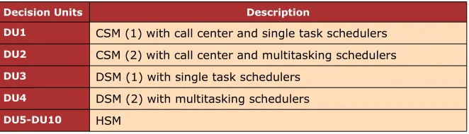
Decision Units Description
DU1 CSM (1) with call center and single task schedulers
DU2 CSM (2) with call center and multitasking schedulers
DU3 DSM (1) with single task schedulers
DU4 DSM (2) with multitasking schedulers
DU5-DU10 HSM
Table 2. Configuration generation for the major scheduling models.
The mean time between arrivals of appointments is 2 minutes and follows exponential distribution. Service time follows triangular distribution. The distributions for service time and arrival of appointment request are obtained from analyzing the historical data.
Decision Units HSM Cluster1 Cluster2 Cluster3
DU5 HSM (1) Lab, primary one, urology Lab, primary two, physicaltherapy Lab, Audiology
DU6 HSM (2) Lab, primary one, primary two Urology, audiology Physical therapy
DU7 HSM (3) Lab, primary one, primary two Lab, urology, physical therapy Audiology
DU8 HSM (4) Lab, primary one, primarytwo, urology Audiology, Physical Therapy
DU9 HSM (5) Lab, primary one, urology,physical Therapy Lab, primary2, audiology
DU10 HSM (6) Lab, primary one, Audiology,urology Lab, primary2, Physicaltherapy
Decision Unit Model Average Waiting Time (hour)
Average Total time (hour)
Average Utilization rate
Number of Staffs
DU1 CSM (1) 0.00925 0.05119 0.42 3
DU2 CSM (2) 0.00925 0.05119 0.6 3
DU3 DSM (1) 0.0549 0.1424 0.43 5
DU4 DSM (2) 0.0549 0.1424 0.65 5
DU5 HSM (1) 0.1111 0.1723 0.62 3
DU6 HSM (2) 0.0867 0.1506 0.53 3
DU7 HSM (3) 0.0777 0.1424 0.51 3
DU8 HSM (4) 0.02823 0.0903 0.47 2
DU9 HSM (5) 0.03184 0.0874 0.48 2
DU10 HSM (6) 0.0414 0.0999 0.49 2
Table 4. Simulation outputs for the setting with high interaction
5.2. Configuration generation
Different configurations of the three major PAS models of CSM, DSM, and HSM are generated. They are considered as decision units for DEA models. The configurations in this study include: two CSMs, two DSMs, and six HSMs. The first CSM includes a call center and the schedulers are single task. The second CSM, does not include a call center and the schedulers are multitasking. As a result for the second CSM, the utilization of the schedulers is multiplied by a coefficient to obtain the correct value for utilization of staff for performing scheduling task. The third and forth configurations are DSM. Six configurations for HSM are also developed that assign clinics to different clusters and each cluster has its own scheduler. All configurations are summarized in Table 2 and Table 3.
5.2.1. Simulation outputs
Decision Unit Model Average Waiting Time (hour)
Average Total time (hour)
Average Utilization rate
Number of Staffs
DU1 CSM (1) 0.003032 0.0320 0.41 3
DU2 CSM (2) 0.003032 0.0320 0.6 3
DU3 DSM (1) 0.01268 0.0545 0.2 5
DU4 DSM (2) 0.01268 0.0545 0.4 5
DU5 HSM (1) 0.01882 0.05236 0.33 3
DU6 HSM (2) 0.016034 0.04856 0.256 3
DU7 HSM (3) 0.0186 0.05390 0.3 3
DU8 HSM (4) 0.03066 0.06604 0.419 2
DU9 HSM (5) 0.02368 0.05525 0.387 2
DU10 HSM (6) 0.00599 0.03573 0.3 2
Table 5. Simulation outputs for the setting with medium interaction
5.2.2. Validation/Verification
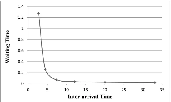
Model validation is measured through evaluating how accurate the created model depicts the real system Sensitivity analysis is applied to validate the simulation model through changing the inter-arrival between appointment requests and proportion of multiple appointments.
The inter-arrival time is changed from 1 to 3.5 and the behavior of average waiting time before connecting to a scheduler as well as average holding time are captured. Figure 2 and Figure 3 show the obtained waiting time and holding time by the simulation model. As it is observed, both waiting time and holding time are decreased by increasing the inter-arrival time. This matches the expectation.
Figure 3. The impact of request arrival on holding time
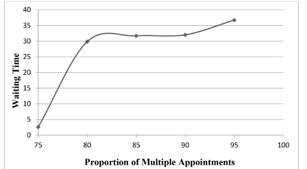
The proportion of multiple appointments is changed from 75 to 95 percent and the behavior of average waiting time before connecting to a scheduler as well as average holding time are captured. Figure 4 and Figure 5 show the obtained waiting time and holding time by the simulation model. As it is observed, both waiting time and holding time are increased by increasing the proportion of multiple appointments. This matched the expectation.
Figure 5. Impact of proportion of multiple appointments on holding time
Decision Unit Model Average Waiting
Time (hour) Average Total time(hour) Average Utilizationrate Number of Staffs
DU1 CSM (1) 0.002372 0.0288 0.3 3
DU2 CSM (2) 0.002372 0.0288 0.5 3
DU3 DSM (1) 0.006516 0.036227 0.35 5
DU4 DSM (2) 0.006516 0.036227 0.65 5
DU5 HSM (1) 0.014799 0.0421904 0.25 3
DU6 HSM (2) 0.011171 0.038508 0.21 3
DU7 HSM (3) 0.0172 0.045078 0.21 3
DU8 HSM (4) 0.0171 0.04487 0.2 2
DU9 HSM (5) 0.01942 0.04619 0.2 2
DU10 HSM (6) 0.0033 0.028 0.21 2
Table 6. Simulation outputs for the setting with low interaction
5.3. Results
5.3.1. Analyze inefficient configurations
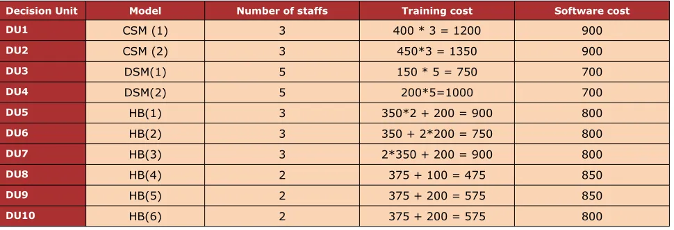
Decision Unit Model Number of staffs Training cost ($) Software cost ($)
DU1 CSM (1) 3 400 * 3 = 1200 900
DU2 CSM (2) 3 450*3 = 1350 900
DU3 DSM (1) 5 150 * 5 = 750 700
DU4 DSM (2) 5 200*5=1000 700
DU5 HSM (1) 3 350*2 + 200 = 900 800
DU6 HSM (2) 3 350 + 2*200 = 750 800
DU7 HSM (3) 3 2*350 + 200 = 900 800
DU8 HSM (4) 2 375 + 100 = 475 850
DU9 HSM (5) 2 375 + 200 = 575 850
DU10 HSM (6) 2 375 + 200 = 575 800
Table 7. DEA inputs for the setting with high interaction
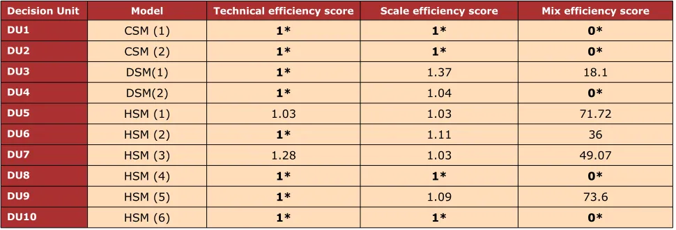
Equations (1)-(5) are applied to evaluate technical efficiency. Configurations 5 and 7 are technically inefficient. This indicates the scheduling software and the schedulers do not use their available capability.
Equations (6)-(9) are applied to evaluate scale efficiency. Scale inefficiency in the configurations 3, 5, 6, 7 and 9 shows that the complexity of scheduling software and schedulers’ skill level in DSM and HSM are not sufficient and improvement is needed in terms of scheduling software and schedulers’ skills.
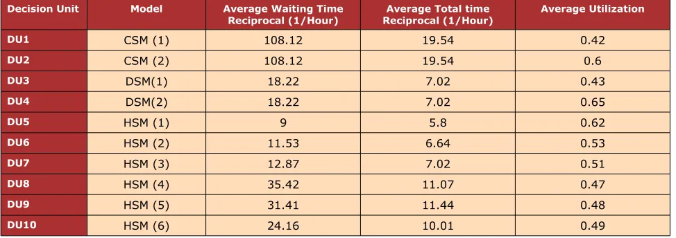
Decision Unit Model Average Waiting Time
Reciprocal (1/Hour) Reciprocal (1/Hour)Average Total time Average Utilization
DU1 CSM (1) 108.12 19.54 0.42
DU2 CSM (2) 108.12 19.54 0.6
DU3 DSM(1) 18.22 7.02 0.43
DU4 DSM(2) 18.22 7.02 0.65
DU5 HSM (1) 9 5.8 0.62
DU6 HSM (2) 11.53 6.64 0.53
DU7 HSM (3) 12.87 7.02 0.51
DU8 HSM (4) 35.42 11.07 0.47
DU9 HSM (5) 31.41 11.44 0.48
DU10 HSM (6) 24.16 10.01 0.49
Decision Unit Model Technical efficiency score Scale efficiency score Mix efficiency score
DU1 CSM (1) 1* 1* 0*
DU2 CSM (2) 1* 1* 0*
DU3 DSM(1) 1* 1.37 18.1
DU4 DSM(2) 1* 1.04 0*
DU5 HSM (1) 1.03 1.03 71.72
DU6 HSM (2) 1* 1.11 36
DU7 HSM (3) 1.28 1.03 49.07
DU8 HSM (4) 1* 1* 0*
DU9 HSM (5) 1* 1.09 73.6
DU10 HSM (6) 1* 1* 0*
Table 9. Inefficiency terms for the setting with high interaction level
Finally, Equations (10)-(19) are applied to evaluate mix inefficiency. Mix inefficiency in configuration 3, 5, 6, 7 and 9 is an evidence for the presence of extra inputs and outputs’ shortfalls.
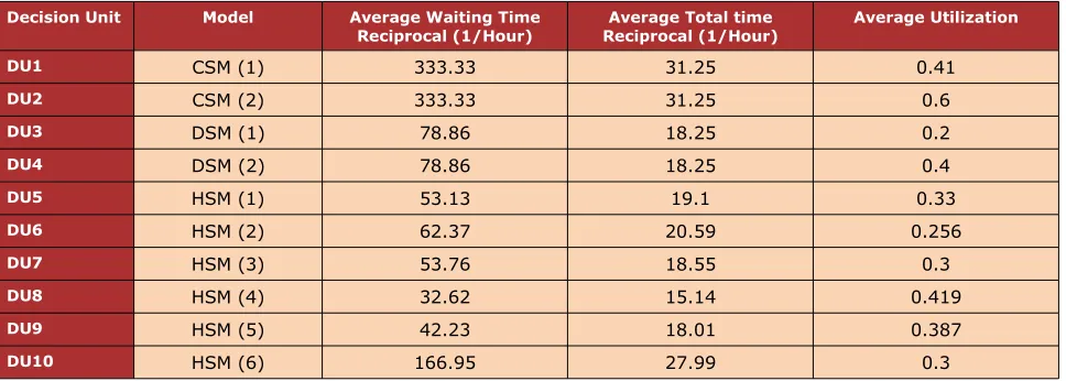
The DEA inputs and outputs value for the setting with medium interaction level are illustrated in Table 10 and Table 11. Table 12 presents the results from analyzing different terms of inefficiency for the clinic setting with medium interaction level.
Decision Unit Model Number of staffs Training cost Software cost
DU1 CSM (1) 3 400 * 3 = 1200 900
DU2 CSM(2) 3 450*3=1350 900
DU3 DSM(1) 5 150 * 5 = 750 700
DU4 DSM(2) 5 200*5=1000 700
DU5 HSM (1) 3 350*2 + 200 = 900 800
DU6 HSM (2) 3 350 + 2*200 = 750 800
DU7 HSM (3) 3 2*350 + 200 = 900 800
DU8 HSM (4) 2 375 + 100 = 475 850
DU9 HSM (5) 2 375 + 200 = 575 850
DU10 HSM (6) 2 375 + 200 = 575 800
Decision Unit Model Average Waiting Time
Reciprocal (1/Hour) Reciprocal (1/Hour)Average Total time Average Utilization
DU1 CSM (1) 333.33 31.25 0.41
DU2 CSM (2) 333.33 31.25 0.6
DU3 DSM (1) 78.86 18.25 0.2
DU4 DSM (2) 78.86 18.25 0.4
DU5 HSM (1) 53.13 19.1 0.33
DU6 HSM (2) 62.37 20.59 0.256
DU7 HSM (3) 53.76 18.55 0.3
DU8 HSM (4) 32.62 15.14 0.419
DU9 HSM (5) 42.23 18.01 0.387
DU10 HSM (6) 166.95 27.99 0.3
Table 11. DEA outputs for the setting with medium interaction
Equations (1)-(5) are applied to evaluate technical efficiency. Configurations 5 and 7 are technically inefficient that indicates the scheduling software and the schedulers do not use their capability. Equations (6)-(9) are applied to evaluate scale efficiency. Scale inefficiency in the configurations 3, 4, 5, 6, 7 and 9 shows that the complexity of scheduling software and schedulers’ skill level are not sufficient and improvement is needed in terms of scheduling software and schedulers’ skills.
Decision Unit Model Technical efficiency score Scale efficiency score Mix efficiency score
DU1 CSM(1) 1* 1* 0*
DU2 CSM(2) 1* 1* 0*
DU3 DSM(1) 1* 1.3 132.97
DU4 DSM(2) 1* 1.33 232.76
DU5 HSM (1) 1.35 1.06 179.56
DU6 HSM (2) 1* 1.15 174.26
DU7 HSM (3) 1.39 1.06 188.57
DU8 HSM (4) 1* 1* 0*
DU9 HSM (5) 1* 1.09 143
DU10 HSM (6) 1* 1* 0*
Decision Unit Model Number of staffs Training cost Software cost
DU1 CSM (1) 3 400 * 3 = 1200 900
DU2 CSM (2) 3 450*3 = 1350 900
DU3 DSM(1) 5 150 * 5 = 750 700
DU4 DSM(2) 5 200*5=1000 700
DU5 HB(1) 3 350*2 + 200 = 900 800
DU6 HB(2) 3 350 + 2*200 = 750 800
DU7 HB(3) 3 2*350 + 200 = 900 800
DU8 HB(4) 2 375 + 100 = 475 850
DU9 HB(5) 2 375 + 200 = 575 850
DU10 HB(6) 2 375 + 200 = 575 800
Table 13. DEA inputs for the setting with low interaction
Finally, Equations (10)-(19) are applied to evaluate mix inefficiency. Mix inefficiency in configurations 3, 4, 5, 6, 7 and 9 is an evidence for the presence of extra inputs and output shortfalls. The DEA inputs and outputs value for the setting with low interaction level are illustrated in Table 13 and Table 14. Table 15 presents the results from analyzing different terms of inefficiency for the clinic setting with low interaction level.
Decision Unit Model Average Waiting Time
Reciprocal (1/Hour) Reciprocal (1/Hour)Average Total time Average Utilization
DU1 CSM(1) 434.79 35.71 0.3
DU2 CSM(2) 434.79 35.71 0.5
DU3 DSM(1) 192.31 31.25 0.35
DU4 DSM(2) 192.31 31.25 0.65
DU5 HB(1) 66.67 25 0.25
DU6 HB(2) 133.33 29.94 0.21
DU7 HB(3) 188.68 32.26 0.21
DU8 HB(4) 454.54 35.71 0.2
DU9 HB(5) 500 37.04 0.2
DU10 HB(6) 303.03 35.7 0.21
Table 14. DEA outputs for the setting with low interaction level
Decision Unit Model Technical efficiency score Scale efficiency score Mix efficiency score
DU1 CSM (1) 1.02 1.08 0*
DU2 CSM (2) 1* 1* 0*
DU3 DSM (1) 1* 1* 0*
DU4 DSM (2) 1* 1* 0*
DU5 HSM (1) 1.4 1.01 324.7
DU6 HSM (2) 1.04 1* 58.7
DU7 HSM (3) 1.1 1* 385.67
DU8 HSM (4) 1* 1* 0*
DU9 HSM (5) 1.07 1.06 142
DU10 HSM (6) 1* 1* 0*
Table 15. Inefficiency terms for the setting with low interaction
Equations (6)-(9) are applied to evaluate scale efficiency. 10 runs and 10 comparisons of the model are performed to identify scale efficient configuration(s). Scale inefficiency in the configurations 1, 5, and 9 shows the complexity of scheduling software and schedulers’ skill level in these two configurations are not sufficient and improvement should be applied in the scheduling software and schedulers’ skills.
Finally, Equations (14)-(19) are applied to evaluate mix inefficiency. The mix inefficient configurations are identified through 20 runs of model. Mix inefficiency in configurations 5, 6, 7 and 9 is an evidence for the presence of extra inputs and outputs’ shortfalls.
5.3.2. Identify efficient configurations
5.3.2.1. Clinic setting with high interaction level
The configuration is identified as efficient if it is efficient in terms of technical, scale and mix. 20 comparisons are done between terms of efficiency. Table 9 shows that the efficient configurations for clinic setting with high interaction level are: DU1, DU2, DU8, and DU10.
5.3.2.2. Clinic setting with medium interaction level
5.3.2.3. Clinic setting with low interaction level
The efficient configurations for clinic setting with low interaction level are: DU1, DU2, DU3, DU4, DU8, and DU10.
5.3.3. Selecting the most efficient configuration
5.3.3.1. Clinic settings with high interaction level
Equations (20)-(24) are applied to remove unrealistic efficient configurations through minimax efficiency approach. Table 16 presents the results for selecting the most efficient configuration in the clinic setting with high interaction level. The DEA model runs 10 times and configuration 2 is identified as the most efficient configuration. This indicates in the presence of high proportion of multiple appointments advanced information sharing system and multi-tasking schedulers with high skill level are required.
The properties of the most efficient configuration for the setting with high interaction level are presented in Table 17. Single tasking versus multitasking is one of the major differences between configurations 1 and 2. Configuration 2 with multitasking option is applicable if the schedulers’ utilization in configuration 1 is less than 50 percent. In a case the utilization is smaller than 50 percent, a coefficient should be multiplied to the schedulers’ utilization in the first configuration to obtain the second configuration’s utilization. In the second configuration 6 staffs do the task of 9 staffs (3 schedulers and 6 check-in staffs), so there is 0.33 percent ((6-9)/9) decrease in staffs number that makes staffs’ utilization (42 percent) increase to 60 percent.
Decision Unit Model Minimax efficiency score
DU1 CSM (1) 0.75
DU2 CSM (2) 1*
DU3 DSM (1) 0.65
DU4 DSM (2) 0.9
DU5 HSM (1) 0.78
DU6 HSM (2) 0.83
DU7 HSM (3) 0.69
DU8 HSM (4) 0.62
DU9 HSM (5) 0.73
DU10 HSM (6) 0.72
Scheduling Model Configuration Type Average Waiting
Time (Hour) Average total time(Hour) UtilizationAverage CSM(2) CSM with multitasking staffs andwithout scheduling center 33 sec 3 min 0.6
Table 17. Properties of final configuration for settings with high interaction level.
5.3.3.2. Clinic settings with medium interaction level
Equations (20)-(24) are applied to remove unrealistic efficient configurations. The minimax efficiency approach selects the two Configurations 2 and 10 as efficient configurations. Therefore, modified minimax efficiency approach with k equal to 0.25 is applied to determine the most efficient configuration. Configuration 10 is selected as the most efficient configuration.
Configuration 10 with HSM decision structure outweighs configuration 2 with CSM decision structure in terms of lower cost. In the presence medium proportion of multiple appointments in the current clinic setting, it is efficient to form two clusters and assign the clinics with high interaction level to the same clinic with CSM decision structure. Configuration 10 provides sufficient accessibility and resource utilization besides lower cost. Table 18 presents the results for selecting the most efficient configuration in the clinic setting with medium interaction level.
Decision Unit Model MiniMax efficiency score efficiency score of M – 0.25*d0
DU1 CSM (1) 0.89 0.72
DU2 CSM (2) 1* 0.864
DU3 DSM (1) 0.628 0.628
DU4 DSM (2) 0.64 0.65
DU5 HB (1) 0.678 0.678
DU6 HB (2) 0.823 0.789
DU7 HB (3) 0.65 0.65
DU8 HB (4) 0.62 0.62
DU9 HB (5) 0.69 0.69
DU10 HB (6) 1* 1*
Table 18. Selecting the most efficient configuration for the setting with medium interaction
Scheduling Model Configuration Type Average Waiting Time
(Hour) Average total time(Hour) Average Utilization
HSM(6) HSM with 2 cluster 22 sec 2.14 min 0.7
Table 19. Properties of final configuration for settings with medium interaction level.
5.3.3.3. Clinic settings with low interaction level
Equations (20)-(24) are applied to select the most efficient configuration through minimax efficiency approach. Configurations 4 and 10 are selected. Therefore, the modified minimax efficiency approach with k equal to 0.25 is applied and configuration 4 is selected as the most efficient configuration. Configuration 4 has DSM decision structure outweighs configuration 10 with HSM decision structure in terms of lower cost. Table 20 presents the results for selecting the most efficient configuration in the clinic setting with low interaction level.
Decision Unit Model MiniMax efficiency score Efficiency score of M – 0.25*d0
DU1 CSM (1) 0.95 0.75
DU2 CSM (2) 0.89 0.78
DU3 DSM (1) 0.9 0.7
DU4 DSM (2) 1* 1*
DU5 HSM (1) 0.88 0.7
DU6 HSM (2) 0.87 0.94
DU7 HSM (3) 0.73 0.73
DU8 HSM (4) 0.74 0.74
DU9 HSM (5) 0.71 0.71
DU10 HSM (6) 1* 0.99
Table 20. Selecting the most efficient configuration for the setting with low interaction
The properties of the configuration that is selected as the most efficient one for the setting with low interaction level are presented in Table 21.
Scheduling Model Configuration Type Average Waiting Time
(Hour) Average total time(Hour) Average Utilization
DSM(2) Multitasking staffs 23 sec 2.17 min 0.65
6. Conclusion
This study focuses on developing a framework, which integrates simulation study with DEA approach, to determine the most efficient PAS model and its configuration for a specific healthcare setting. The efficiency is determined based on three terms of: technical efficiency, scale efficiency, and mix efficiency. Technical efficiency presents scheduling software and schedulers’ performances match their capability. Scale efficiency shows complexity of the scheduling software and skill level of schedulers match the clinic setting context. Finally, the mix inefficiency indicates the presence of extra inputs and outputs’ shortfalls. The configuration is efficient if it has all the three terms of efficiency simultaneously.
A case study for different types of healthcare settings is conducted to illustrate the effectiveness of the proposed method. The case study shows, the most efficient PAS For the clinic setting with high interaction level is the CSM. For the healthcare setting with medium interaction level is the HSM. For the clinic setting with low interaction level is the DSM (the schedulers are multitasking). The most efficient scheduling models for the three clinic settings in the case study are selected in terms of the balance between patient satisfaction, schedulers’ utilization and scheduling system cost.
The developed framework in this study can be used for any real world healthcare setting. When different healthcare setting is studied, new simulation models should be developed to obtain the DEA outputs. The most efficient configuration for the new setting is determined through the developed DEA approach in this study.
For the future work, further simulation study will be conducted to determine the mutual impact of scheduling model and clinic flows. Queuing theory will be applied to determine the required resource for different configuration. Additional inputs and outputs will be defined to apply in the DEA approach to select the most efficient PAS model.
References
Agnihotri, S., & Taylor, P. (1991). Staffing a centralized Appointment Scheduling Department in Lourdes Hospital. Interfaces, 21(5), 1-11. http://dx.doi.org/10.1287/inte.21.5.1
Al-Refaie, A., Fouad, R.H., Li, M.H., & Shurrab, M. (2014). Applying simulation and DEA to improve performance of emergency department in a Jordanian hospital. Simulation Modelling Practice and Theory, 41, 59-72. http://dx.doi.org/10.1016/j.simpat.2013.11.010
Berry, J., & Phanthasomchit, S. (2000). Centralized and Decentralized Scheduling Using HL7.
Canadian Institute of Health Information.
Cooper, W., Seiford, L.M., & Tone, K. (2006). Introduction to Data Envelopment Analysis and its usesa. New York: Springer Science Business Media.
Ertay, T., & Ruan, D. (2005). Data envelopment analysis based decision model for optimal operator allocation in CMS. European Journal of operational Research, 164(3), 800-810.
http://dx.doi.org/10.1016/j.ejor.2004.01.038
Ertay, T., Ruan, D., & Tuzkaya, U.R. (2006). Integrating data envelopment analysis and analytic hierarchy for the facility layout design in manufacturing systems. Information Science,
176(3), 237-262. http://dx.doi.org/10.1016/j.ins.2004.12.001
Guo, M., Wagner, M., & West, C. (2004). Outpatient Clinic Scheduling- A Simulation Approach.
Proceedings of the 36th Conference On Winter Simulation, 1981-1987.
Gupta, D., & Denton, B. (2008). Appointment scheduling in health care: Challenges and opportunities. IIE transactions, 40(9), 800-819. http://dx.doi.org/10.1080/07408170802165880
Hooten, M.E., & U.S. ARMY Academy of Health Sciences. (1990). An effective outpatient appointment system for General Leonard Wood Army Community Hospital. Master’s Thesis. A v a i l a b l e a t : http://www.dtic.mil/cgi-bin/GetTRDoc? Location=U2&doc=GetTRDoc.pdf&AD=ADA237807
Jacobson, S.H., Hall, S.N., & Swisher, J.R. (2013). Discrete-event simulation of health care systems. In Patient Flow, pp. 273-309. Springer US. http://dx.doi.org/10.1007/978-1-4614-9512-3_12
Lai, M.C., Huang, H.C., & Wang, W.K. (2010). Designing a knowledge-based system for benchmarking: A DEA approach. Knowledge-Based Systems, 24(5), 1-10.
Li, X.B., & Reeves, G.R. (1999). A multiple criteria approach to data envelopment analysis.
European Journal of Operational Research, 115(3), 507-517. http://dx.doi.org/10.1016/S0377-2217(98)00130-1
Mustafee, N., Katsaliaki, K., & Taylor, S. J. (2010). Profiling literature in healthcare simulation.
Simulation, 86(8-9), 543-558. http://dx.doi.org/10.1177/0037549709359090
Nealon, J., & Moreno, A. (2003). Agent-Based Application in Health Care. In Applications of Software Agent Technology in the Health Care Domain, pp. 3-18. Birkhäuser Basel.
Peng, Q., Niu, Q., & ElMekkawy, T.Y. (2013). Improvement in the Operating Room Efficiency Using Tabu Search in Simulation. Business Process Management Journal, 19(5), 3-3.
Shim, S.J., & Kumar, A. (2010). Simulation for emergency care process reengineering in hospitals. Business Process Management Journal, 16(5), 795-805.
http://dx.doi.org/10.1108/14637151011076476
Venkatesh, B. (2006). Technical Efficiency Measurement by Data Envelopment Analysis: An Application in Transportation. Alliance Journal of Business Research, 2(1), 60-72.
Weng, S.J., Tsai, B.S., Wang, L.M., Chang, C.Y., & Gotcher, D. (2011, December). Using simulation and data envelopment analysis in optimal healthcare efficiency allocations. In Proceedings of the Winter Simulation Conference, pp. 1295-1305. Winter Simulation Conference.
Yang, T., & Kuo, C. (2003). A hierarchical AHP/DEA methodology for the facility layout design problem. European Journal of Operational Research, 147(1), 128-136.
http://dx.doi.org/10.1016/S0377-2217(02)00251-5
Zhang, J., Dharmadhikari, N., & Song, D. (2009). Literature Review on Centralized and Decentralized Scheduling. Fargo, ND: Department of Industrial and Manufacturing Engineering.
Zhang, J., Gonela, V., & Aslani, N. (2010). Develop a decision tool for a hospital/clinic setting to decisde whether to schedule in a Centralized or Decentralized manner. Fargo, ND: Department of Industrial and Manufacturing Engineering, NDSU.
Zhang, J., Gonela, V., & Aslani, N. (2011). Development of Centralized, Decentralized and Hybrid Scheduling Model. Fargo, ND: Department of Industrial and Manufacturing Engineering, NDSU.
Journal of Industrial Engineering and Management, 2014 (www.jiem.org)
Article's contents are provided on a Attribution-Non Commercial 3.0 Creative commons license. Readers are allowed to copy, distribute and communicate article's contents, provided the author's and Journal of Industrial Engineering and Management's names are included.