Vol.9 (2019) No. 5
ISSN: 2088-5334
A Comparison of Supervised Learning Techniques for Predicting the
Mortality of Patients with Altered State of Consciousness
Muhammad Ariff Yasri
#1, Shamimi A. Halim
#2, Muthukkaruppan Annamalai
#3 #Faculty Computer and Mathematical Science, Universiti Teknologi MARA, Shah Alam, Selangor, 40450, Malaysia E-mail: [email protected]; [email protected]; [email protected]
Abstract— The study attempts to identify a potentially reliable supervised learning technique for predicting the outcomes of mortality in an altered state of consciousness (ASC) patients. ASC is a state distinguished from ordinary waking consciousness, which is a common phenomenon in the Emergency Department (ED). Thirty (30) distinctive attributes or features are commonly used to recognize ASC. The study accordingly applied these features to model the prediction of mortality in ASC patients. Supervised learning techniques are found to be suitable for such classification problems. Consequently, the study compared five supervised learning techniques that are commonly applied to evaluate the risk of mortality using health-related datasets, namely Decision Tree, Neural Network, Random Forest, Naïve Bayes, and Logistic Regression. The labeled dataset comprised patient records captured by the Universiti Sains Malaysia hospital’s Emergency Medicine department from June to November 2008. The cleaned dataset was divided into two parts. The larger part was used for training and the smaller part, for evaluation. Since the ratio between training and testing samples varies between individual supervised learning techniques, we studied the performance of the modeled techniques by also varying the proportion of the training data to the dataset. We applied four percentage splits; 66%, 75%, 80%, and 90% to allow for 3-, 4-, 5- and 10-fold cross-validation experiments to evaluate the accuracy of the analyzed techniques. The variation helped to lessen the chance of over fitting, and averaged the effects of various conditions on accuracy. The experiments were conducted in the WEKA environment. The results indicated that Random Forest is the most reliable technique to model for predicting the mortality in ASC patients with acceptable accuracy, sensitivity, and specificity of 70.9%, 76.3%, and 65.5%, respectively. The results are further confirmed by SROC analysis. The findings of the study serve as a fundamental step towards a comprehensive study in the future.
Keywords— supervised learning technique; predictive modelling; mortality; altered state of consciousness.
I. INTRODUCTION
An altered state of consciousness (ASC) is a common emergency case in the emergency department, and it is associated with significant mortality. The exact etiology of ASC is unknown at the clinical point of care. Later, a reliable prognosis is difficult to predict. On the other hand, surgical, medical, and ethical decisions depend upon this information. While it is legitimate to set up optimum medical and therapeutic cares and good prognosis for patients, it may not be desirable for medical teams to promote such treatments when the predictable prognosis is poor. A better understanding of patients’ outcomes would help in decisions related to rehabilitation, acute or end-of-life care to reduce the in-hospital death risk.
Quick and accurate prediction of mortality for patients with ASC is essential to ensure immediate appropriate actions or interventions in emergency departments. Prediction systems that can learn from collected data have the potential to offer rapid and reliable prognostic information for medical teams’ decision-making.
Machine learning allows computers to learn and analyze the pattern without explicitly being programmed [1]. Two main types of machine learning techniques are supervised and unsupervised. Supervised learning technique can be regarded as a learning function that maps an input to an output based on the labeled training dataset. The training set (input-output pairs) can be extracted from existing electronic medical records. On the other hand, unsupervised learning look toward unlabeled data and tries to learn the patterns in the data without any training. When labeled dataset is available, supervised learning techniques are applied because they make it possible to test the predictive model.
The rest of the paper is organized as follows. Section II describes the research material and method. The results and discussion are given in section III, and the study is concluded in section IV. The section briefly describes ASC and symptoms related to it, machine learning in healthcare, and the supervised learning process before moving on to the related works.
A. The Altered States of Consciousness
Altered State of Consciousness (ASC) is a general phrase to describe the state of awareness of one’s self and environment [3]. It is an altered mental status describing the undifferentiated presentation of disorders of mentation such as imbalanced cognition and reduced awareness [4]. Patients fall under the ASC due to lifestyle causes (e.g., consumption of alcohol, toxin and drug [5]) and triggered by health conditions (e.g., trauma, hypoglycemia, and stroke [6]). For this reason, the demographic, lifestyle, and clinical information are used to evaluate risks in ASC patients. The number of patients presented at ED with ASC indicates a low prevalence of less than 6% of the total patient arrivals [7]. The low incidence is also acknowledged in our Malaysian study. Therefore, data is collected over a protracted period to have sufficient data to conclude.
B. Machine Learning in Healthcare
The amount of data generated exponentially today lends great opportunity for industries to utilize them to optimize their operations. The healthcare industry is dealing with this growing data trend. Healthcare datasets tend to capture patient data such as age, gender, race, vital sign readings, diagnosis, and so on, which are multivariate [8]. The collected data has the potential to uncover clinically relevant patterns and meaning in data [9]. Machine learning techniques have made mining patterns in large dataset possible. The knowledge discovered in the data can be translated to actionable information for evidence-based medicine. They can also be the source for predicting indications and warnings to improve clinical outcomes.
Naïve Bayes (NB), Logistic Regression (LR), Decision Tree (DT), Random Forest (RF), Neural Network (NN), Classification Tree (CT), K-Nearest Neighbor (KNN) and Support Vector Machine (SVM) are prevalent machine learning techniques used for predictive modeling. These techniques are commonly applied on health-related and non-health related datasets [27], as well as on mortality prediction from clinical data [8]. The applications of these techniques in the health-related dataset are presented in section II (D).
C. Supervised Learning Process
The machine learning techniques mentioned in the previous section are examples of supervised learning techniques, which are well suited for predictive modeling. The supervised learning process comprises data collection and feature selection, data preparation, model development, model evaluation and model deployment [10], [11].
1) Data collection: It is a step of gathering various data
from different sources in a systematic way that enables to test hypotheses and answer research questions. The data can be in structured, semi-structured, or unstructured form.
2) Feature Selection: It is a move to select significant
features, reducing the dimensionality of data if necessary. The high dimensional dataset can affect the accuracy of the prediction model. Chi-Squared, Entropy-Based, and Correlation filtering are some of the methods used for finding significant features in data.
3) Data Preparation: It is the most critical step in the
supervised learning process. Based on previous researches, we list four main data preparation activities, i.e., cleaning, formatting, sampling, and re-sampling of the data. Data cleaning is an activity of removing or imputing the inaccurate, incomplete, or unreasonable data to correct errors, detect, and analyze outliers [12]. Case Deletion, Mean Imputation, and Median Imputation are some of the suggested methods for replacing missing values in the dataset [13]. Data formatting is converting or translating a data into its respective format such as converting a date string into a standard date format for the data to be analysed correctly. Data sampling relates to splitting of the data into training and testing sets. In general, at least two-third (66%) of the data is set aside for training in a reasonably sized dataset of more than one hundred cases or records [14], but larger training dataset will allow a model to learn more possible patterns of the problem. Incidentally, a lower percentage split can be more biased in some cases, and a higher percentage split can suffer from large variability in other cases. A seemingly apropos train: test percentage split is subject to the data sample and the supervised learning technique employed. This is apparent in previous researches, which have reported different train: test percentage splits for good results. For example, the application of supervised learning in an Engineering problem applied a 70-percentage split (70:30 split) [15]; in a Stock price prediction problem, 80-percentage split (80:20 split) was used [16]; and, when cross-validation was applied, as high as 90-percentage split (90:10 split) has been suggested [17]. Data resampling is carried out to facilitate model validation. The decision based on a single held-out split of the dataset is not regarded as a rigorous validation, especially when the size of the data sample is small. A small data sample will compel an even smaller test set that will give cause to error induced by bias, and render the result inconclusive. Therefore, k-fold cross-validation is often applied to validate model performance on limited data sample [17]. The cross-validation is an extension of the train: test percentage split, where the data sample is randomly divided into k disjoint partitions of equal size, and each part has roughly the same class distribution. Subsequently, the model is trained k times; each time on k-1 partitions and the model is tested on the remaining partition. The resampling procedure ensures that every case from the data sample has the same chance of appearing in the training and test sets, and the averaged result produced is unbiased.
(whether by duplication or by interpolation of synthetic samples) applies bias to increase the chance of training minority class cases. An alternative to avoid the data distortion is to collect more minority class cases when possible, to present a more balanced perspective on the classes.
4) Model Development: The step follows Data
Preparation. The development of a machine-learning model can be initiated by comparing the performance of several supervised learning techniques, then select one and implement it. The preferred technique can be further tuned to the quirks of the training dataset. Machine-learning platforms and tools can help to prototype a model that implements a technique, and subsequent configuration and coding can dwell into the depth of the technique [19].
5) Model Evaluation: It is a step to evaluate the
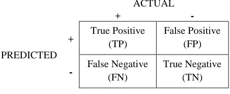
performance of a machine-learning model. Three common performance metrics of a predictive model, especially in the healthcare setting are accuracy, sensitivity, and specificity [20]. The formulas for calculating these metrics refer to the predicted vs. actual outcomes confusion matrix shown in Figure 1.
ACTUAL
+ -
PREDICTED
+ True Positive (TP)
False Positive (FP)
- False Negative (FN)
True Negative (TN)
Fig. 1. Confusion Matrix
Accuracy is a quintessential performance metrics. Equation 1 shows the formula for calculating accuracy. Average Accuracy finds the average of the accuracy results obtained from several cross-validation experiments, as Equation 2 describes. Because Accuracy does not distinguish between false positives and false negatives, the Sensitivity and Specificity metrics are considered. Sensitivity calculates the TP rate, while specificity calculates the TN rate. Equations 3 and 4 give the formulas for Sensitivity and Specificity, respectively.
Accuracy, a = (TP + TN) / (TP + FN + TN + FP) (1)
Average Accuracy = ∑ (2)
Sensitivity = TP / (TP + FN) (3)
Specificity = TN / (TN + FP) (4)
It is desirable to have a predictor with high sensitivity and specificity, which however is often difficult to achieve in practice without compromising one for the other.
6) Model Deployment: It is the final step to integrate the
machine-learning model into the current system or set-up as a new system.
D. Related Works
The existence of many supervised learning techniques is a testament that there is no “one size fit all” technique that can be relied upon for data analytics. The nature, quality and size of data, as well as the problem to be solved often determines the technique of choice. Data can be numerical, categorical or a mixture of both. LR and NN techniques are promising choices for numerical data, while techniques like CT is a potential choice for categorical data. However, we can be certain of the supervised learning options for mixed data. Because most health-related dataset involves a mixture of numerical and categorical data, it is therefore not surprising that different technique is selected to model prediction on different disease datasets. In a research conducted on the Cleveland Clinic Foundation dataset and Statlog dataset to predict heart disease where the majority of the data variables are categorical, DT is said to outperform the other techniques by as much as 99% accuracy [21]. SVM has been shown to perform better in detecting brain tumor using linear Magnetic Resonance Imaging (MRI) tumor data [22]. The research compared NB, DT, SVM and NN, and SVM has the highest accuracy of 93.8%.
Supervised learning techniques do benefit from large data size. In general, when more training data is used, the predictive power of the techniques will increase [23]. Moreover, more training is required when there are more features to learn from. Even though plenty of data may be available, much of the data may not be useful if its quality of the data is bad. To ensure successful prediction, the training data must be relatively ‘clean,’ i.e., accurate, complete, and consistent [12]. Therefore, pre-processing of data that include dimensionality reduction (cf. Feature Selection), dealing with missing values and sampling (cf. Data Preparation), is a significant contributing factor for meaningful prediction. For example, in a research that focused on prediction of mortality, several supervised learning techniques were compared using health and fitness data [24]. In this instance, over-sampling of the imbalanced data resulted in marked improvements in the performance of KNN, DT, and RF to deliver predictions. Nevertheless, as mentioned in section II (C), over-sampling may not necessarily be an option to address all cases of imbalanced data.
Different application problems involving the same dataset can end-up choosing different supervised learning techniques. For example, in the Healthcare Cost and Utilisation Project [8], five different techniques, i.e., LR, NN, DT, NB, and SVM were compared to predict readmission and mortality of newly admitted patients. The study identified the NN technique as a reliable predictor of mortality, whereas the LR technique was found to be a better predictor of readmission.
II. MATERIALS AND METHOD
The section describes the material and method applied to comparatively analyze and identify a potentially reliable supervised learning technique for predicting the mortality of patients with ASC.
A. Data Collection and Feature Selection
The dataset comprises three hundred and four (304) instances collected by doctors in the Department of Emergency Medicine in Hospital Universiti Sains Malaysia (HUSM), Kubang Kerian. The targets are the unconscious patients arriving at the Red zone. Because of the low incidence of ASC, the data was collected over six months, from June to November 2008. The instances capture three categories of data organized according to the demographic, lifestyle, and clinical information, i.e., the commonly used
attributes or features for recognizing ASC. Tables I, I, and III list these features and their corresponding statistics.
TABLEI DEMOGRAPHIC INFORMATION
Feature Value Statistics
Age Number Age = 13 – 85;
Mean = 56.3 ± 16.9 years Race Malay, Chinese or
Others
Malay = 197; Chinese = 16; Others = 6
Gender Male or Female Male = 119; Female = 100
TABLEII LIFESTYLE INFORMATION
Feature Value Statistics
Smoking Yes or No Yes = 72; No = 147
Alcohol consumption
Yes or No Yes = 4; No = 215
TABLEIII CLINICAL INFORMATION
Feature Value Statistics
Hypertension Yes or No Yes = 128; No = 91
Diabetes Mellitus Yes or No Yes = 69; No = 150
Ischemic heart disease Yes or No Yes = 42; No = 177
Atrial Fibrillation Yes or No Yes = 6; No = 213
Chronic Heart Disease Yes or No Yes = 3; No = 216
Asthma Yes or No Yes = 24; No = 195
Renal Disease Yes or No Yes = 25; No = 194
Epilepsy Yes or No Yes = 12; No = 207
Duration of symptom Number Mean = 11.6 ± 16.9 days
Heart Rate Number Mean = 93.8 ± 27.7 bpm
Systolic Blood Pressure Number Mean = 148.3 ± 46.9 mmHg
Diastolic Blood Pressure Number Mean = 82.4 ± 26.4 mmHg
Temperature Number Mean = 37.3 ± 0.7 C
Glasgow Coma Scale Number Mean = 10.3 ± 3.4 points
Neck Stiffness Yes or No Yes = 18; No = 201
Papilloedema Yes or No Yes = 13; No = 206
Pupillary Reflex Bilateral Reactive,
Unilateral Unreactive or Bilateral Unreactive
Bilateral Reactive = 204 Unilateral Unreactive = 2 Bilateral Unreactive = 13
Doll’s sign Yes or No Yes = 216; No = 3
Reflexes Normal,
Unilateral Hyperreflexia, Bilateral Hyperreflexia, Unilateral Hyporeflexia or Bilateral Hyporeflexia
Normal = 103
Unilateral Hyperreflexia = 33 Bilateral Hyperreflexia = 15 Unilateral Hyporeflexia = 21 Bilateral Hyporeflexia = 47
White Blood Count Number Mean = 12.2 ± 5.7 x 10⁹/L
Red Blood Sugar Number Mean = 9.4 ± 6.7 mmol/L
Arterial Blood Gas Normal,
Mixed Picture, Respiratory Alkolosis, Metabolic Alkolosis, Respiratory Acidosis or Metabolic Acidosis
Normal = 89 Mixed Picture = 31 Respiratory Alkolosis = 1 Metabolic Alkolosis = 9 Respiratory Acidosis = 13 Metabolic Acidosis = 76
Intubation Yes or No Yes = 67; No = 152
Babinski Test Normal,
Unilateral Upgoing, Bilateral Upgoing, Equivocal Unilateral or Equivocal Bilateral
Normal = 105
Unilateral Upgoing = 57 Bilateral Upgoing = 23 Equivocal Unilateral = 17 Equivocal Bilateral = 17
B. Data Preparation
Removing doubtful instances from the original dataset cleans the data. Eighty-five (85) instances were removed from the original dataset based on six (6) exclusion criteria set by the doctors:
1) Patients admitted with psychiatric illnesses,
hallucination and bizarre behavior are deemed to have a normal level of consciousness;
2) Patients twelve (12) years old and younger are
regarded children; their Glasgow Coma Scale is difficult to assess, and some are unable to comprehend certain commands;
3) Patients with ASC more than 72 hours since only
Glasgow Coma Scale scores at the onset of ASC are analyzed;
4) Patients with loss of consciousness secondary to cough,
micturition, and migraine because these conditions are usually due to abnormalities in autonomic functions;
5) Patients with ASC secondary to terminal or end-stage
diseases because these patients have generally a fluctuating level of consciousness.
6) Patients with recurrent episodes of ASC during the
data collection period caused by the same etiology.
The removal of these instances also helps to eliminate outliers in the dataset. The outcome of the analysis is a binary status of the patient, i.e., ‘Alive’ or ‘Dead.’ Out of the two hundred and nineteen (219) instances in the cleansed dataset, one hundred and eighteen (118) instances have ‘Alive’ and one hundred and one (101) instances have ‘Dead’ status; a reasonably balanced dataset.
Next, missing values are replaced so that they can be fed into the model. Case deletion is not suitable for our dataset because removing instances with missing values will further reduce the size of an already small dataset. We used Median Imputation instead. Table IV shows a snapshot of the ASC data with few instances that have missing values denoted as NULL.
TABLEIV
SNAPSHOT OF SAMPLE ASCDATA WITH NULL VALUES
For each column with missing values, the corresponding median of the observed values is calculated, and this value is used to replace the missing values.
C. Model Development and Comparison
Five supervised machine-learning techniques are selected for comparison. They are Logistic Regression (LR), Neural Network (NN), Naïve Bayes (NB), Decision Tree (DT), and Random Forest (RF).
LR is a non-linear technique that can be applied to categorical data to classify cases. NN is a graph-like classifier constructed using weighted ‘neurons’ with the ability to learn from its errors. NB is a technique based on a statistical model that applies conditional probability to classify cases. DT uses binary recursive partitioning to construct a classification tree, which is similar to people’s decision process. RF takes the wisdom of the crowd to make its prediction by combining the results from multiple DTs.
According to previous researches (see section II (D)), these five machine learning techniques are suitable for predictive modeling and are best applied to a dataset containing multiple input variables composed of both numerical and categorical features, and output that takes two discrete values (Y/N), such as our case. The experiments are conducted in the WEKA environment [19] using the default parameters of each technique.
Following the practice of previous researches, we applied four percentage splits of the data: 66%, 75%, 80%, and 90%, with the number of data partitions k equal to 3, 4, 5, and 10, respectively. For each percentage split experiment, we would repeat k rounds of cross-validation, three (3) times for each partition. To reduce the risk of bias, we randomly assigned data into the k partitions each time. Therefore, we will have (3 * k) results of prediction accuracies for each percentage split experiment has been trained and tested on a different partition of the data sample every round and every time. In the end, we combine the results by averaging them to estimate the final accuracy for the percentage split.
The multiple cross-validations of the supervised learning technique using different training dataset sizes is performed to fairly analyze the reliability of the individual supervised learning technique in a small data sample. The performance of the predictive model is based on the final accuracy, which is supported by the sensitivity and specificity measures. The metrics are founded on the predicted and actual mortality outcomes. The formulas of these metrics are given in section II (C).
III.RESULTS AND DISCUSSION
A. Results
We present the results of the experiments and compare the performance of the five supervised learning techniques selected to model the prediction of mortality for patients with ASC.
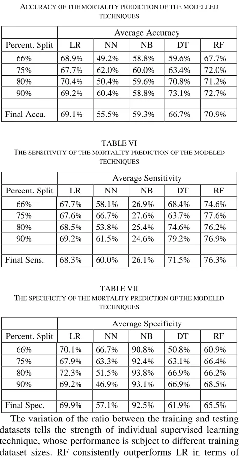
Table V shows the average accuracy of each modelled technique for each percentage split experiment, and their corresponding final accuracy (i.e., the average of the average percentage split accuracies) on the last row. The sensitivity and specificity of the experiments are presented in the same manner in the following tables. Table VI shows the results of average sensitivity for each percentage split experiment and the final sensitivity of each modelled technique, while Table VII shows the average specificity for each percentage split
C
H
D
A
st
h
m
a
R
en
al
E
p
ile
p
sy
D
u
r
H
R
S
B
P
D
B
P
T
em
p
G
C
S
2 1 2 2 4 110 235 150 37 14
2 2 1 2 12 73 180 51 37 14
2 1 2 2 0.8 134 176 110 37 13
2 2 2 1 3 100 130 80 37 10
2 2 2 2 24 126 NULL NULL 37 12
2 2 2 2 21 NULL NULL NULL 37.5 7
experiment and the final specificity of each modelled technique.
Our experiments show that RF, LR and DT are potentially reliable techniques for predicting the mortality outcome in ASC patients. RF is the best performer with accuracy, sensitivity, and specificity of 70.9%, 76.3%, and 65.5% respectively. LR (69.1% accuracy, 68.3% sensitivity and 69.9% specificity) and DT (66.7% accuracy, 71.5% sensitivity and 61.9% specificity) closely follow it. However, LR demonstrates a higher specificity than RF and DT, which mean LR can predict the ‘Alive’ outcomes, i.e., the TN rate more accurately than the latter.
TABLEV
ACCURACY OF THE MORTALITY PREDICTION OF THE MODELLED TECHNIQUES
Average Accuracy
Percent. Split LR NN NB DT RF
66% 68.9% 49.2% 58.8% 59.6% 67.7% 75% 67.7% 62.0% 60.0% 63.4% 72.0% 80% 70.4% 50.4% 59.6% 70.8% 71.2% 90% 69.2% 60.4% 58.8% 73.1% 72.7%
Final Accu. 69.1% 55.5% 59.3% 66.7% 70.9%
TABLEVI
THE SENSITIVITY OF THE MORTALITY PREDICTION OF THE MODELED TECHNIQUES
Average Sensitivity
Percent. Split LR NN NB DT RF
66% 67.7% 58.1% 26.9% 68.4% 74.6% 75% 67.6% 66.7% 27.6% 63.7% 77.6% 80% 68.5% 53.8% 25.4% 74.6% 76.2% 90% 69.2% 61.5% 24.6% 79.2% 76.9%
Final Sens. 68.3% 60.0% 26.1% 71.5% 76.3%
TABLEVII
THE SPECIFICITY OF THE MORTALITY PREDICTION OF THE MODELED TECHNIQUES
Average Specificity
Percent. Split LR NN NB DT RF
66% 70.1% 66.7% 90.8% 50.8% 60.9% 75% 67.9% 63.3% 92.4% 63.1% 66.4% 80% 72.3% 51.5% 93.8% 66.9% 66.2% 90% 69.2% 46.9% 93.1% 66.9% 68.5%
Final Spec. 69.9% 57.1% 92.5% 61.9% 65.5% The variation of the ratio between the training and testing datasets tells the strength of individual supervised learning technique, whose performance is subject to different training dataset sizes. RF consistently outperforms LR in terms of accuracy and sensitivity from the 75% split. Similarly, RF also outperforms DT in terms of accuracy and sensitivity at all percentage splits except at the 90% split where DT happens to perform better than the rest. The accuracy of DT is relatively weak below the 80% split though, which contributed to its lower averages. Meanwhile NB and NN are the laggards, with accuracy less than 60%.
B. Discussion
The purpose of identifying of mortality risk in ASC patients is to guide immediate appropriate actions or interventions, and consequently reduce the risk of in-hospital death. Therefore, we prioritize sensitivity (the TP rate) over specificity in our study. A sensitive predictor will miss few cases of mortality risk due to less false negatives. In this regards, RF, LR and DT have emerged as promising ‘inclusive’ techniques for predicting the mortality of patients with ASC. These modelled techniques have shown to have modest prediction accuracy and sensitivity that averages around 70% value. In contrast, NB is the most ‘restrictive’ technique of all.
As the performances of RF, LR and DT are close to one another, a Summary Receiver Operating Characteristics (SROC) analysis was performed to draw distinction among them. The SROC curve is essentially a TP rate vs. FP rate plot (see Figure 2). TP rate is the sensitivity value, while FP rate is (1 - Specificity) value. An ideal predictor will have TPR value 1 and FPR value 0 (i.e., top left hand corner), while the worst predictor will have TPR value 0 and FPR value 1 (i.e., bottom right hand corner).
SROC is suitable for comparative analysis of accuracy of various predictors using a single data sample [25], such as in our case where the different modelled techniques apply a common sample data, test variables, method, and other controlled study qualities. We also applied a common acceptance threshold of 50% for all the modelled techniques compared in this study. Accordingly, we connected the outer boundary coordinates involving NB, LR and RF to shape the SROC curve as shown in Figure 2.
Fig. 2. Summary Receiver Operating Characteristics of the Techniques
RF is in the paramount position on the SROC curve, and LR is close second on the curve. DT is not far from RF and LR, but is located below the curve. NB is on the curve but is clearly biased to ‘negative’ outcomes. NN is approaching the ‘average’ diagonal, which performs somewhat like a random predictor.
Previous studies have found that the accuracy of RF and LR increase with dimensions [26]. Besides, tree-based techniques such as RF and DT are found to perform better than LR when a large dataset is used [26]. Thus, the small data sample size of the study appears to have contributed to the better-than-expected performance of LR.
In view of the fact that RF is an ensemble of DTs, we believe RF will perform even better on a large data sample that allows it to build superior DTs. Apparently the accuracy of the tree-based techniques increases with the increase in size of the training set (see Tables V). Another advantage of the tree-based techniques is their transparency [28]. These techniques make explicit the traces to conclusion, and also reveal the variables that significantly influence the prediction outcome. The information will be useful for feature selection and refinement that can help to build strong prediction models – a scope for future work.
NN is biased towards numerical data. For that reason, NN’s fair performance may be attributed to the large number of categorical variables used in our study. In addition, the results show that NN’s accuracy fluctuates across different percentage splits. The inconsistent performance could be due to the way NN is simulated in the WEKA environment.
It is interesting to note that NB’s accuracy hovers consistently near 60% across the different percentage splits, yet it admits too many false negatives as evident by its poor sensitivity of 26.1%. NB underestimates the mortality risk, which does not augur well for the goal of our study that warrants inclusive consideration in the life-threatening situation in Emergency Departments. NB assumes strong independence condition among variables [22]. NB’s underperformance implies that the naïve assumption may not be tenable in our study.
IV.CONCLUSION
The study sets to identify a potentially reliable supervised learning technique for determining the outcomes of mortality in ASC patients. Five supervised learning techniques were comparatively analyzed. The study finds that the techniques based on discriminative models, namely RF, LR and DT are suitable for predicting the mortality risks in ASC patients. In contrast NB, which is a generative model, performed poorly.
RF with the highest accuracy and sensitivity emerged as the dominant technique that can be relied upon to predict the mortality of patients with ASC. We believe RF’s performance will be boosted when a larger dataset is used. Because RF is an ensemble of DTs and its result is a generalized vote from the many DTs, a larger data size allows it to build superior DTs.
Finally, we regard the findings of the study as preliminary to be confirmed in future work through increased data sample size and fine-tuning. It will also be necessary to evaluate further variants and implementations of the techniques.
ACKNOWLEDGEMENT
The authors thankfully acknowledge Universiti Teknologi MARA (UiTM) for support of this work, which was funded under the Ministry of Education’s Fundamental Research Grant Scheme (ref. no. FRGS/1/2016/ICT01/UITM/02/3).
The authors also express their gratitude to the Department of Emergency Medicine in Hospital Universiti Sains Malaysia (HUSM), Kubang Kerian for their contribution to the data collection.
REFERENCES
[1] R. C. Deo, “Machine Learning in Medicine”, Circulation, vol. 132, pp. 1920–1930, 2015.
[2] A. Ławrynowicz and V. Tresp, Introducing Machine Learning. Perspectives on Ontology Learning, AKA Heidelberg, 2014. [3] R. Ahmad and M. Masilamany, Non-Traumatic Altered States of
Consciousness, Lambert Academic Publishing, Berlin, 2010. [4] W. Kanich, W. J. Brady, J. S. Huff, A. D. Perron, C. Holstege, G.
Lindbeck and C. T. Carter, “Altered Mental Status: Evaluation and Etiology in the ED,” American Journal of Emergency Medicine, vol. 20, no. 7, pp. 613–617, 2002.
[5] D. Vaitl, N. Birbaumer, J. Gruzelier, G. Jamieson, B. Kotchoubey, A. Kubler and T. Weiss, “Psychobiology of Altered States of Consciousness,” Psychology of Consciousness: Theory, Research, and Practice, vol. 1, pp. 2-47, 2013.
[6] P. Lai, G. Yiang, M. Tsai and S. Hu, “Analysis of Patients with Altered Mental Status in an Emergency Department of Eastern Taiwan,” Tzu Chi Medical Journal, vol. 21, no. 2, pp. 151–155, 2009. [7] J. L. Song, V. J. Wang and M. N. Vasquez, “Altered Level of
Consciousness: Evidence-based Management in the Emergency Department,” Pediatr Emerg Med Pract, vol. 14, no. 1, 2017. [8] M. Almardini and Z. W. Raś, A Supervised Model for Predicting the
Risk of Mortality and Hospital Readmissions for Newly Admitted Patients, LNCS, 2017, vol. 10352.
[9] F. Prior, “Medical Knowledge Discovery and Management,” Journal of Military Medicine, vol. 5, no. 21, pp. 21–26, 2009.
[10] D. Simona and M. Michael, “Churn analysis - Machine learning,” Indiana University, Project Report, 2017.
[11] C. E. Sapp, “Preparing and architecting for machine learning,” Gartner Technical Professional Advice, 2017.
[12] A. J. Tallón-Ballesteros and J. C. Riquelme, Data Cleansing Meets Feature Selection: A Supervised Machine Learning Approach, J. Ferrandez Vicente, J. Alvarez-Sanchez, F. de la Paz Lopez, F. Toledo-Moreo and H. Adeli Eds., LNCS, Cham: Springer, 2015, vol. 9108.
[13] E. Acuña and C Rodriguez, The Treatment of Missing Values and its Effect on Classifier Accuracy, D. Banks, F.R. McMorris, P. Arabie and W. Gaul, Eds., Classification, Clustering, and Data Mining Applications Studies in Classification, Data Analysis and Knowledge Organisation. Berlin: Springer, 2004.
[14] K. K. Dobbin and R. M. Simon, “Optimally Splitting Cases for Training and Testing High Dimensional Classifiers,” BMC Medical Genomics, vol. 4, no. 1, 2011.
[15] M. A. Shahin, H. R. Maier and M. B. Jaksa, “Data Division for Developing Neural Networks Applied to Geotechnical Engineering,” Journal of Computing in Civil Engineering, vol. 18, no. 2, pp. 105– 114, 2004.
[16] B. W. Wanjawa, “Predicting future Shanghai stock market price using ANN in the period 21-Sep-2016 to 11-Oct-2016,” Preprint arXiv:1609.05394, 2016.
[17] S. Borra and A. Di Ciaccio, “Measuring the Prediction Error: A Comparison of Cross-Validation, Bootstrap and Covariance Penalty Methods,” Computational Statistics & Data Analysis, vol. 54, no.12, pp. 2976–2989, 2010.
[18] N. V. Chawla, Data Mining for Imbalanced Datasets: An Overview, O. Maimon and L. Rokach, Eds., Data Mining and Knowledge Discovery Handbook. Boston: Springer, 2005.
[19] S. B. Aher and L. M. R. J Lobo, “Data mining in educational system using weka,” in Proc. ICEET’11, pp. 20–25.
[20] E. Gladstone, K. Smolina, S. G. Morgan, K. A. Fernandes, D. Martins and T. Gomes, “Sensitivity and Specificity of Administrative Mortality Data for Identifying Prescription Opioid-related Deaths,” Canadian Medical Association Journal, vol. 188, no. 4, pp. 67–72, 2016.
[22] J. Varun and G. Sunila, “Comparative Study of Data Mining Classification Methods in Brain Tumor Disease Detection,” International Journal of Computer Science & Communication, vol. 8, no. 2, pp. 12–17, 2017.
[23] S. Venkataraman, “System design for large scale machine learning,” University of California, Berkeley, Tech. Rep. UCB/EECS-2017-219, 2017.
[24] S. Sakr, R. Elshawi, A. M. Ahmed, W. T. Qureshi, C. A. Brawner, S. J. Keteyian and M. H. Al-Mallah, “Comparison of Machine Learning Techniques to Predict All-Cause Mortality using Fitness Data: The Henry Ford Exercise Testing (FIT) Project,” BMC Medical Informatics and Decision Making, vol. 17, no. 1, 2017.
[25] C. M. Jones and T. Athanasiou, “SROC Analysis Techniques in the Evaluation of Diagnostic Tests,” Annals of Thoracic Surgery, vol. 79, pp. 16–20, 2005.
[26] R. Couronne, P. Probst and A. Boulesteix, “Random Forest versus Logistic Regression: A Large-scale Benchmark Experiment,” BMC Bioinformatics, vol. 19, no. 270, 2018.
[27] S. Zainudin, D. S. Jasim and A. A. Bakar, “Comparative Analysis of Data Mining Techniques for Malaysian Rainfall Prediction,” International Journal on Advanced Science, Engineering and Information Technology, vol. 6, no. 6, pp. 1148–1153, 2016. [28] F. E. Sapri, N. S. Nordin, S. M. Hasan, W. F. W. Yaacob and S.