A New High Frequency Grid Impedance Estimation Technique for the Frequency Range of 2 to150 kHz

(1)

Please cite this article as: M.M. AlyanNezhadi, H. Hassanpour, F. Zare, A New High Frequency Grid Impedance Estimation Technique for the Frequency Range of 2 to150 kHz, International Journal of Engineering (IJE), IJE TRANSACTIONS A: Basics Vol. 31, No. 10, (October 2018) 1666-1674

International Journal of Engineering

J o u r n a l H o m e p a g e : w w w . i j e . i r

A New High Frequency Grid Impedance Estimation Technique for the Frequency

Range of 2 to150 kHz

M. M. AlyanNezhadi*a_{, H. Hassanpour}a_{, F. Zare}b

a Image Processing and Data Mining Lab, Shahrood University of Technology, Shahrood, Iran b Power Engineering Group, University of Queensland, Queensland, Australia

P A P E R I N F O

Paper history:

Received 28 May 2018

Received in revised form 12 August 2018 Accepted 17 August 2018

Keywords: Impedance Estimation Frequency Response Discrete Fourier Transform Power Quality

Smart Grids

A B S T R A C T

Grid impedance estimation is used in many power system applications such as grid connected renewable energy systems and power quality analysis of smart grids. The grid impedance estimation techniques based on signal injection uses Ohm’s law for the estimation. In these methods, one or several signal(s) is (are) injected to Point of Common Coupling (PCC). Then the current through and voltage of PCC are measured. Finally, the impedance is assumed as ratio of voltage to current signals in frequency domain. In a noisy system, energy of the injected signal must be sufficient for an accurate approximation. However, power quality issues and regulations limit the energy and the voltage levels of the injected signal. There are three main issues in impedance estimation using signal injection: I) Power quality of grid, II) frequency range of estimation, and finally III) accuracy of estimation. In this paper, the stationary wavelet denoising algorithm is employed instead of increasing the energy of injection signal(s). In the paper, a novel method is proposed for impedance estimation based on selecting several appropriate injection signals and denoising the measured signals. The proposed method is able to impedance estimation in a wide frequency range without any effect on power quality. Finally, simulation results have been carried out to validate the proposed method.

doi: 10.5829/ije.2018.31.10a.08

1. INTRODUCTION1

Electrical impedance is assumed as the ratio of voltage signal of Point of Common Coupling (PCC) to current through PCC in frequency domain [1, 2]. The impedance of the grid consists of inductive, resistive and capacitive couplings is dependent on the type and configuration of grid elements such as transformers and feeders. The grid impedance is measured in frequency domain and it varies at different frequencies. Impedance estimation is used in many applications such as islanding detection [3, 4], controlling the stability of the current controller [5], designing the stable inverter [6], passive and active filter design [7, 8], and improving the performance of the impedance-source converter [9]. Impedance estimation techniques use the Ohm’s law in

*Corresponding Author Email: alyan.nezhadi@gmail.com (M. M. AlyanNezhadi)

frequency domain. Impedance estimation techniques can be categorized into passive [10, 11] and active [6, 12, 13] methods. Passive methods estimate the impedance of grid with no effect on power quality of the network because they estimate the grid impedance without changing or injecting a signal to the grid. In the passive methods, the current through and voltage of PCC are measured, and then the impedance is approximated based on the Ohm’s law. They are able to estimate grid impedance only at the frequencies that are present in the sampling time. Since usually the normal active grids have one main frequency (frequencies of 50 or 60 Hz) and its harmonics, these methods are unable to estimate the impedance at various frequencies once the grid distortions are not enough [14]. In addition, passive grids do not have any main frequency. Therefore, these methods are unable to impedance estimation.

(2)

grid power quality once energy of the injecting signal is high [14]. On the other hand, the accuracy of impedance estimation in these methods is high. In addition, the active methods can estimate high frequency impedance when grid is live and connected to a voltage source.

The techniques that use signal injection for grid impedance estimation can be categorized to estimation in single frequency and frequency range. For impedance estimation in frequency 𝑓, we can inject sinusoidal pulse with frequency 𝑓 and calculate the devision of voltage to current of PCC at frequency 𝑓 [5].

In literature, different researchers used various signals such as impulse [15], chirp [13], pseudo-random binary sequence, Maximum Length Binary Sequence [16], several short term impulse signals [17] and sequence of rectangular pulses [18] for a wide frequency impedance estimation. One of the simplest ways is the injection of several sinusoidal pulses in various frequencies and estimating the impedance by interpolation. This method needs several signal injections and therefore reduces the power quality of grid. We can use a wideband injection signal such as impulsive signal for impedance estimation in wide frequency range.

The existing international technical documents and standards cover all grid connected electrical and electronic systems for the frequency up to 2 kHz based on IEC 61000-3-2, IEC 61000-3-12 and IEEE 519 standards. In addition, there is a CISPR standard for frequencies above 150 kHz. Our researches show that there is no harmonic compatibility levels for the frequency range of 2-150 kHz. This frequency range is the most important issue for the International Standardization Committee (IEC, TC77A).

In 2015, the IEC-TC77A-WG8 proposed a compatibility limit in the frequency range 2-30 kHz while a compromise for non-intentional emissions in the frequency range 30-150 kHz has not been reached [1, 19-21]. Compatibility levels are defined based on harmonics emission and immunity levels of grid connected equipment. Thus, knowledge of grid impedance characteristics over the frequency range of 2-150 kHz is very important to estimate the level of distortion caused by grid connected equipment.

Grid impedance estimation is used for a new harmonic emission and immunity, which has been discussed at international levels. Major international companies have been working to develop some documents for power quality control of future grids but it is a lack of grid impedance to understand how power quality of the grids are affected. Hence, we investigate impedance estimation in low voltage grids.

AlyanNezhadi et al. [17] tried to increase the accuracy of impedance estimation using optimization of the injection signals. In this paper, we added a new denoising stage for more accurate impedance

estimation. Therefore, the accuracy of impedance estimation with the proposed method (with the same injection signals) is higher than the results of the one introduced in [17].

2. GRID IMPEDANCE ESTIMATION

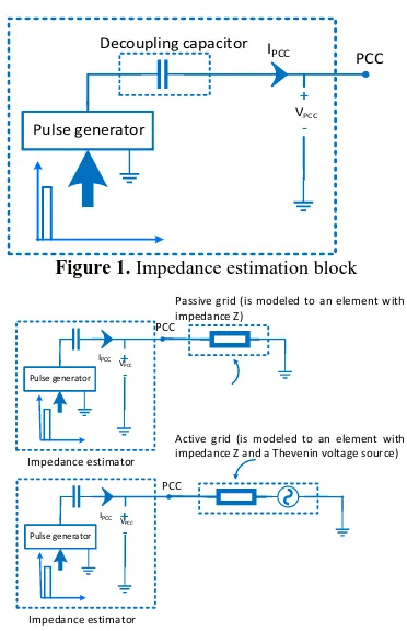
As aforementioned, impedance of every point in the grid is assumed as ratio of voltage to current signal in frequency domain, according to the Ohm's law. Therefore, for impedance estimation in frequency 𝑓, the voltage or current signal must have a component at frequency 𝑓. Hence, for having an arbitrary component frequency, we can inject a voltage or current signal to the grid. The block shown in Figure 1 can be used to estimate the impedance of PCC.

In noisy systems, the accuracy of estimation is dependent to energy of injected signal. Therefore, for an accurate estimation in frequency 𝑓, the injected signal must have sufficient energy in the frequency 𝑓 [2]. One of the most important injection signals is rectangular pulse. Energy of rectangular injection pulse is dependent to two parameters, maximum peak amplitude and pulse width. Maximum peak amplitude of the rectangular injection pulse is controlled up to 2kV. Increasing the pulse width causes increasing the energy of injection signal. However, it reduces the bandwidth of the pulse and therefore estimation cannot be done accurately in the frequencies with low energy.

2. 1. Active and Passive Grid Impedance Estimation Since passive grids do not have any power generator, the whole impedance of the passive grid seen from PCC can be assumed as an element with impedance 𝑍𝑔.

For impedance estimation of the passive grid, the impedance estimation block must be connected to the grid as shown in Figure 2. Based on the Ohm's law, the impedance seen from the PCC is equal to:

𝑍𝑔(𝑓) =

𝑉𝑃𝐶𝐶(𝑓)

𝐼𝑃𝐶𝐶(𝑓) (1)

where 𝑉𝑃𝐶𝐶(𝑓) and 𝐼𝑃𝐶𝐶(𝑓) are respectively voltage of and current through PCC in frequency domain. For impedance estimation at the specified frequency 𝑓𝜆, the injection signal must contain the same frequency component 𝑓𝜆; in the mathematical equation, 𝑉𝑃𝐶𝐶(𝑓𝜆) ≠

0. Accordingly, selection of injection signal is important.

(3)

PCC

IPCC

VPCC

+

-Decoupling capacitor

Pulse generator

Figure 1. Impedance estimation block

PCC

IPCC _V

PCC

+ -Pulse generator

Impedance estimator PCC

IPCC_V

PCC

+ -Pulse generator

Impedance estimator

Passive grid (is modeled to an element with impedance Z)

Active grid (is modeled to an element with impedance Z and a Thevenin voltage source)

Figure 2. Schematic of impedance estimation for passive and

active grids

𝑍𝑔(𝑓) =

𝑉𝑃𝐶𝐶(𝑓)−𝑉𝑇ℎ𝑒𝑣𝑒𝑛𝑖𝑛(𝑓)

𝐼𝑃𝐶𝐶(𝑓) (2)

where 𝑉𝑃𝐶𝐶(𝑓), 𝐼𝑃𝐶𝐶(𝑓) and 𝑉𝑇ℎ𝑒𝑣𝑒𝑛𝑖𝑛(𝑓) are respectively voltage of and current through PCC and Thevenin voltage of grid in frequency domain. Since measurement of Thevenin voltage of grid is difficult [23], the use of this equation is not effective [24]. One way to use the above equation is the synchronized estimation of Thevenin voltage and impedance of grid. We can estimate the grid impedance using below equation:

𝑍𝑔(𝑓) =

𝑉_{𝑃𝐶𝐶,𝑛1}(𝑓)−𝑉_{𝑃𝐶𝐶,𝑛2}(𝑓)

𝐼𝑃𝐶𝐶,𝑛1(𝑓)−𝐼𝑃𝐶𝐶,𝑛2(𝑓) (3)

where 𝑉𝑃𝐶𝐶,𝑛_𝑖(𝑓) and 𝐼𝑃𝐶𝐶,𝑛_𝑖(𝑓) are respectively voltage of and current through PCC for injections 𝑖 = 1,2 in frequency domain. Active grid impedance estimation can be done by two separate injections (where 𝑡2≅ 𝑡1) using the above equation. However, for impedance estimation at frequency 𝑓𝜆, 𝑉𝑃𝐶𝐶,𝑛1(𝑓𝜆) ≠ 𝑉𝑃𝐶𝐶,𝑛2(𝑓𝜆).

The pulse generator in Figure 1 can be replaced by a ground connection instead of second injection. Therefore, Equation (3) is simplified to:

𝑍𝑔(𝑓) =

𝑉𝑃𝐶𝐶(𝑓)−𝑉𝑃𝐶𝐶𝐺𝑁𝐷(𝑓)

𝐼𝑃𝐶𝐶(𝑓)−𝐼𝑃𝐶𝐶𝐺𝑁𝐷(𝑓)

(4)

where 𝐼𝑃𝐶𝐶𝐺𝑁𝐷(𝑓) and 𝑉𝑃𝐶𝐶𝐺𝑁𝐷(𝑓) are the depletion current and voltage of PCC. Usually the normal grids have one main frequency (frequencies of 50 or 60 Hz) and its

harmonics in the working time; therefore, normal grids have passive behavior in most frequencies.

The main aim of the impedance estimation in low voltage grids is to estimate impedance on high frequency. Hence, the grid impedance at 50Hz or 60Hz is not important but an active grid has a background noise in some harmonics.

2. 2. Impedance Estimation with Additive Noise The errors in impedance estimation can be categorized into measurement error and grid noise. Measurement noise can be modeled by additive white Gaussian noise [2]. In this section, we investigate effects of additive noise (such as measurement error) on the accuracy of impedance estimation. Figure 3 shows schematic of applying the additive measurement noise in a power grid.

Suppose that measured 𝑣𝑃𝐶𝐶,𝑒(𝑡) and 𝑖𝑃𝐶𝐶,𝑟(𝑡) signals have additive noise 𝑒(𝑡) and 𝑟(𝑡), respectively. Based on the Ohm’s law, the impedance at PCC is:

𝑍𝑛(𝑓) = 𝑉𝑃𝐶𝐶,𝑒(𝑓) 𝐼𝑃𝐶𝐶,𝑟(𝑓)=

𝑉𝑃𝐶𝐶(𝑓)+𝐸(𝑓)

𝐼𝑃𝐶𝐶(𝑓)+𝑅(𝑓) 

Therefore the APE would be:

𝐴𝑃𝐸%(𝑓) =

|𝑍(𝑓)−𝑍𝑛(𝑓)|

|𝑍(𝑓)| × 100 

where 𝐴𝑃𝐸%(𝑓) and 𝑍𝑛(𝑓) are APE and the approximated impedance at frequency 𝑓. It is clear that estimation is more accurate when 𝐴𝑃𝐸(𝑓) is close to zero. When impedance estimation is done using a deterministic signal, we can apply the signal to grid repeatedly and calculate the average of estimated impedance in each injection [12, 16]. It can be assumed that the average of noise is zero. Hence, the arithmetic and logarithmic averages of impedances can be used to increase accuracy of approximation and they can be calculated by:

𝑍(𝑓) =1

𝑃∑

𝑉𝑃𝐶𝐶,𝑘(𝑓) 𝐼𝑃𝐶𝐶,𝑘(𝑓) 𝑃

𝑘=1 

𝑍(𝑓) = (∏ 𝑉𝑃𝐶𝐶,𝑘(𝑓) 𝐼𝑃𝐶𝐶,𝑘(𝑓) 𝑃

𝑘=1 )

1 𝑃

 

+

Zgrid

Impedance

Estimator _PCC

Current Measurement

Voltage Measurement

+

iPCC(t)

vPCC(t)

r(t)

e(t)

- +

+

-iPCC,r(t)

vPCC,e(t)

Figure 3. Schematic of applying the additive measurement

(4)

In the above equations, P is the number of injections [12]. Theses equations can be used with different injection signals but using similar injection signals are more efficient.

3. NOVEL IMPEDANCE ESTIMATION METHOD

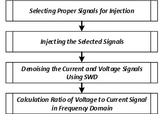
The accuracy of impedance estimation is directly related to energy of injected signal. In this section, we proposed to denoising the current and voltage signals using stationary wavelet denoising (SWD) [25] instead of increasing the energy of the injected signal. The proposed method consists of four main parts, which are described below (see Figure 4).

3. 1. Selecting Proper Signals for Injection The most appropriate signal for injection is impulse (and the extended type of it - rectangular pulse) [2, 15]. The energy of impulse in frequency domain is uniform. In other words, impulse has infinity bandwidth in frequency domain. Ideal impulse has one non-zero sample in discrete domain. Rectangular pulse has two or more non-zero samples in discrete domain and therefore it has not infinity bandwidth in frequency domain. As previously noted, for impedance estimation in noisy systems, the energy of the injected signal must be sufficient for an accurate approximation. Energy of rectangular injection pulse is dependent to peak amplitude and pulse width [2, 17]. Peak amplitude of the injection signal is controlled up to 2kV. In addition, increasing the pulse width reduces the bandwidth of the signal and in the frequencies with low energy (usually in high frequencies), estimation is not accurate [2]. A rectangular pulse 𝑔(𝑡) with peak amplitude 𝐴 and width

𝜁 second can be defined as:

𝑔(𝑡) = {𝐴 0 ≤ 𝑡 ≤ 𝜁

0 𝑂. 𝑊. 

Rectangular pulse 𝑔(𝑡) in frequency domain can be calculated by the Fourier transform of 𝑔(𝑡).

𝔉(𝐺(𝑡)) = {𝐴

𝜔𝑠𝑖𝑛(𝜁𝜔)} + 𝑗 { 𝐴

𝜔(𝑐𝑜𝑠(𝜁𝜔) − 1)}



where 𝔉(.) is the Fourier transform operator. The magnitude spectrum of 𝑔(𝑡) for non-negative frequencies is

|𝔉(𝐺(𝑡))| =2𝐴_𝜔|𝑠𝑖𝑛 (𝜁𝜔₂)| 

The magnitude spectrum of rectangular pulse has periodic and damping behavior. Its spectrum is zero

(𝐺(𝜔) = 0) in below frequencies:

{ 𝜔 =2𝑘𝜋

𝜁 , 𝑘 = 0,1,2, …

𝑓 =𝑘

𝜁, 𝑘 = 0,1,2, …



Selecting Proper Signals for Injection

Injecting the Selected Signals

Denoising the Current and Voltage Signals Using SWD

Calculation Ratio of Voltage to Current Signal in Frequency Domain

Figure 4. The flowchart of the proposed method

Since impedance estimation in frequencies with low energy is not accurate, the authors in the [17] proposed to use several short-term impulsive signals for estimating impedance in a wide frequency range. They determined several injection signals that at least one of the injected signals has sufficient energy in some frequencies that union of these ranges be universal set of estimation for frequencies 2-150 kHz. The suitable signals can be obtained using Genetic algorithm [26, 27]. The proposed injection signals for impedance estimation with measurement noise are given in Figure 5. In this paper, we used four injection signals that they are obtained with the method proposed in our previous publication [17].

3. 2. Injecting the Selected Signals After signal selection, the signals must be injected to the grid separately. The current through and voltage of PCC must be measured in every injection. The sampling time must be sufficient for an accurate impedance estimation.

3. 3. Denoising the Current and Voltage Signals Using SWD When the Signal to Noise Ratio (SNR) of current or voltage signal is near to one, the level of noise and the signal are equal. Therefore, the accuracy of estimation is low. In this paper, we propose to employ SWD to improve the SNR instead of increasing the energy of injection signal. In this level, every current or voltage signals must be denoised. The denoising algorithm has four important stages as stated below:

1. Choosing the mother wavelet. Our simulations show that the sym4 is a suitable mother wavelet for current or voltage signal denoising.

2. Decomposing signal to N levels. Each signal must be decomposed to five levels for denoising process. The number of denoising is selected based on simulations.

3. Thresholding. Selecting an appropriate threshold and applying the soft thresholding, for each level from 1 to N.

(5)

Figure 5. The suggested injection signals in [17]

Quality of denoising dependents on denoising parameters (number of wavelet decomposition levels, wavelet function and thresholding rule ). Hence, the proposed denoising process can be improved via optimizing these parameters. In this paper, these parameters are set experimentally. For automatic parameter regularization, we must have a dataset with many noisy and noiseless current/voltage signals. Then, an evolutionary algorithm such as Genetic algorithm can be used for this purpose.

3. 4. Calculation Ratio of Voltage to Current Signal in Frequency Domain As aforementioned, the ratio of voltage signal to current signal in frequency domain is assumed as impedance. For impedance estimation at each frequency, the injection signal must contain the same frequency components. The best estimation of impedance for specific frequency 𝜔 is done using the injection signal with higher frequency component in this frequency. Therefore, the impedance can be calculated with below equation:

𝑍𝑔(𝑓) =

𝑑𝑒𝑛𝑜𝑖𝑠𝑒𝑑(𝑉𝑃𝐶𝐶(𝑘)(𝑓)−𝑉𝑃𝐶𝐶𝐺𝑁𝐷(𝑓))

𝑑𝑒𝑛𝑜𝑖𝑠𝑒𝑑(𝐼_𝑃𝐶𝐶(𝑘)(𝑓)−𝐼_𝑃𝐶𝐶𝐺𝑁𝐷_(𝑓)) 

𝑘 = 𝑎𝑟𝑔 𝑚𝑎𝑥

1≤𝑔≤𝒦(𝑑𝑒𝑛𝑜𝑖𝑠𝑒𝑑 (𝑉𝑃𝐶𝐶

(𝑘)

(𝑓) − 𝑉_𝑃𝐶𝐶𝐺𝑁𝐷_(𝑓))) _{}

where 𝑉_𝑃𝐶𝐶(𝑘)(𝑓) and 𝐼_𝑃𝐶𝐶(𝑘)(𝑓) are measured voltage of and measured current through PCC for k th injection, respectively. 𝑘 is selected for each frequency based on Equation (14).

4. SIMULATION RESULTS

In this section, many simulations are done on the grid shown in Figure 6. The parameters of the grid in each simulation are different. The proposed method was tested on the grid in different conditions: Case I) grid with low, partial, and full load. Case II) grid with different feeders (underground or overhead cables). Case III) grid impedance estimation from different PCCs. Case IV) grid impedance in day time and night time. In the whole simulations, an additive white

Gaussian noise with 𝑆𝑁𝑅 = 30𝑑𝐵 is assumed as the measurement noise. Each simulation is compared with the methods introduced in literature [17, 28]. AlyanNezhadi et al. [17] used four rectangular injection signals with pulse widths= {7, 11, 14 𝑎𝑛𝑑 26 𝜇𝑠} for impedance estimation. We used a single rectangular pulse, with 26𝜇𝑠 pulse width for impedance estimation as reported in literature [28]. The parameters of the proposed method are summarized in Table 1.

The simulations are done in a computer with Intel(R) Core (TM) i7-6500U, 2.5 GHz and 8 GB RAM with 64 bit Windows 10 operating system. The simulations are done in Matlab/Simulink 2017b Software. In addition, the proposed method was written using Matlab 2017b.

The impedance estimation results are compared using Mean Absolutely Percentage Error (MAPE) [17] and SNR metrics. The reference (actual) impedance is calculated using Matlab/Simulink software. The Simulink software uses the grid model and its parameters (such as the value of each capacitor) and the ideal mathematic formulas.

Building 1 Building 2 Building 3 Building 4 Building 5 Building 6 Building 12

Building 11

Building 10

Building 9

Building 8

Building 7

Building 17 Building 16 Building 15 Building 14 Building 13

Overhead Feeder Cable

Solar system

PCC PCC1

PCC3

P

CC

2

P

ow

er gri

d vol

ta

ge

Figure 6. Schematic of an active grid with three solar systems

for simulations

TABLE 1. Parameters of the proposed method for the

simulations

Element Values

Injection Pulse

Type Rectangular pulse

Number of pulse 4

Width 7, 11, 14 𝑎𝑛𝑑 26 𝜇𝑠

Denoising process

Amplitude 1 kV

Mother wavelet Sym4

Decomposition Levels 5

(6)

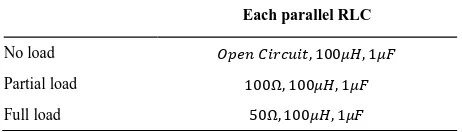
4. 1. Grid Impedance Estimation with Different Loads In this subsection, the impedance of the grid is estimated on three different states (no load, partial and full loads). The parameters of each parallel RLC grid are given in Table 2. The other parameters are the same of those in Table 3. The results are given in Table 4 and Table 5. The obtained results (that are given in Figure 7) show the ability of the proposed method in accurate impedance estimation.

TABLE2. Parameters of schematic grid

Element Values

Each parallel RLC 50Ω, 100𝜇𝐻, 1𝜇𝐹

Each feeder 25𝑚Ω, 30𝜇𝐻, 30𝜇𝐻, 25𝑚Ω

Power grid voltage 220𝑣, 50𝐻𝑧, 𝑝ℎ𝑎𝑠𝑒 0′

Each solar system 𝑠𝑦𝑠𝑡𝑒𝑚 𝑣𝑜𝑙𝑡𝑎𝑔𝑒: 220𝑣, 50𝐻𝑧, 𝑝ℎ𝑎𝑠𝑒 0

′

𝐿𝐶𝐿 𝑓𝑖𝑙𝑡𝑒𝑟: 70𝜇𝐻, 10𝜇𝐹, 200𝜇𝐻

TABLE3.Simulated grid parameters

Each parallel RLC

No load 𝑂𝑝𝑒𝑛 𝐶𝑖𝑟𝑐𝑢𝑖𝑡, 100𝜇𝐻, 1𝜇𝐹

Partial load 100Ω, 100𝜇𝐻, 1𝜇𝐹

Full load 50Ω, 100𝜇𝐻, 1𝜇𝐹

TABLE 4. SNR of impedance estimation for the grid with

different loads

Proposed method

Proposed method in [17]

No load 7.2265 7.1846 6.1832

Partial load 16.985 16.700 11.825

Full load 17.129 16.847 11.647

TABLE 5. MAPE of impedance estimation for the grid with

different loads

No load 2.4041 2.6865 6.1832

Partial load 2.0372 2.3166 11.825

Full load 2.0186 2.2932 11.647

4. 2. Grid Impedance Estimation with Different Feeders In this subsection, the grid impedance is estimated with different feeders. Overhead and underground feeders [29] can be modeled by an RL or LCL model with resistances. In the underground cables,

a capacitive element appears because conductors are located close to each other in the underground. However, nowadays, a dielectric material is located between the conductors [30]. The simulated grid model shown in Figure 6 is used for impedance estimation with two different feeders. The parameters of feeder are given in Table 6. Simulation results show that the proposed method is able to estimate the impedance with overhead and underground feeder cables. The simulation results are given in Tables 7 and 8. The estimated impedances are shown in Figure 8.

a) Estimated impedance with full load

b) Estimated impedance with partial load

c) Estimated impedance with no load

Figure 7. Impedance estimation of grid with full, partial and

no loads

TABLE 6. Simulated parameters of the feeders

Parameters

Underground Feeder Cable 25 𝑚Ω, 75 μH, 500 nF, 75 μH, 25 𝑚Ω

(7)

TABLE 7. SNR of impedance estimation for the grid with different feeders

Proposed method in [17]

Underground Feeder Cable 16.962 16.706 12.457

Overhead Feeder Cable 16.434 16.194 12.615

TABLE 8. MAPE of impedance estimation for the grid with

different feeders

Proposed method in

[17]

Proposed method in

[28]

Underground Feeder Cable 2.0318 2.3016 12.457

Overhead Feeder Cable 2.0723 2.3528 12.615

a) Estimated impedance with overhead feeders

b) Estimated impedance with underground feeders

Figure 8. Impedance estimation of grid with different feeders

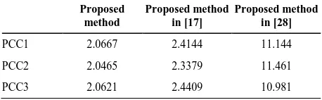
4. 3. Grid Impedance Estimation from Different PCCs The proposed method is able to estimate the impedance from different PCCs. Simulations of this subsection are done in an active grid with three solar systems that is shown in Figure 6 and its parameters is given in Table 2. The results are summarized in Table 9 and Table 10.

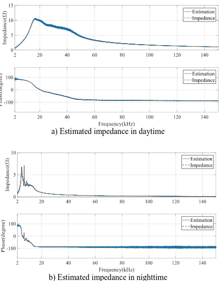
4. 4. Grid Impedance Estimation in Night and Day Times The grid impedance may vary during day and night due to grid side filters (mainly capacitors) of

electrical and electronic equipment and appliances such as efficient lighting systems and battery chargers. Thus, two different load parameters have been considered in this subsection to evaluative the accuracy of the proposed method. The simulations are down on the same grid shown in Figure 6. The parameters of each parallel RLC grid are given in Table 11. The rest of parameters are the same as those in Table 2. The simulation results are given in Table 12 and Table 13. In addition, the estimated impedances in night and day times are given in Figure 9.

TABLE 9. SNR of impedance estimation from different PCCs

PCC1 16.706 16.44 11.144

PCC2 16.768 16.521 11.461

PCC3 16.742 16.454 10.981

TABLE 10. MAPE of impedance estimation from different

PCCs

PCC1 2.0667 2.4144 11.144

PCC2 2.0465 2.3379 11.461

PCC3 2.0621 2.4409 10.981

TABLE 11. Parameters of grid impedance estimation in night

and day times

Each parallel RLC

Daytime 25 Ω, 100 𝜇𝐻, 1𝜇𝐹

Nighttime 25 Ω, 100 𝜇𝐻, 10𝜇𝐹

TABLE 12. SNR of impedance estimation in night and day

times

Daytime 17.323 17.002 11.881

Nighttime 15.666 15.371 11.099

TABLE 13. MAPE of impedance estimation in night and day

times

Daytime 1.9637 2.2401 11.881

(8)

a) Estimated impedance in daytime

b) Estimated impedance in nighttime

Figure 9. Impedance estimation of grid in night and day times

5. CONCLUSIONS

In this paper, a novel grid impedance estimation based on signal processing for frequency range 2-150 kHz is proposed. The focus of this paper is the techniques based on signal injection. Impedance estimation using signal injection follows the Ohm’s law. Accuracy of impedance estimation in noiseless condition is independent to energy of injection signal. On the other hand, in noisy systems, the accuracy of impedance estimation is directly related to energy of injection signal. There are various types of injection signals. One of the main injection signals is rectangular shape pulse. The energy of rectangular pulse is dependent to peak amplitude and pulse width of signal. The peak amplitude is controlled up to 2 𝑘𝑉. In addition, increasing the pulse width leads to decreasing the bandwidth of signal. In this paper, we proposed to use the stationary wavelet de-noising instead of increasing the energy of injected signal. In addition, for wide impedance estimation we used several injection signals in which at least one of the injected signals has sufficient energy in some frequencies and union of these ranges be universal set of estimation. These two modifications cause the more accurate estimation than the previous techniques with the same injection signal. The simulation results show the ability of the proposed method in accurate impedance estimation.

6. REFERENCES

1. Davari, P., Hoene, E., Zare, F., and Blaabjerg, F., “Improving 9-150 kHz EMI Performance of Single-Phase PFC Rectifier”, In Cips 2018 - 10th International Conference on Integrated Power Electronics Systems, VDE-VERLAG, (2018).

2. AlyanNezhadi, M.M., Zare, F., and Hassanpour, H., “Passive grid impedance estimation using several short-term low power signal injections”, In 2nd International Conference of Signal Processing and Intelligent Systems (ICSPIS), IEEE, (2016), 1–5. 3. Ciobotaru, M., Agelidis, V.G., Teodorescu, R., and Blaabjerg, F., “Accurate and Less-Disturbing Active Antiislanding Method Based on PLL for Grid-Connected Converters”, IEEE Transactions on Power Electronics, Vol. 25, No. 6, (2010), 1576–1584.

4. Asiminoaei, L., Teodorescu, R., Blaabjerg, F., and Borup, U., “A Digital Controlled PV-Inverter With Grid Impedance Estimation for ENS Detection”, IEEE Transactions on Power Electronics, Vol. 20, No. 6, (2005), 1480–1490.

5. Ciobotaru, M., Teodorescu, R., and Blaabjerg, F., “On-line grid impedance estimation based on harmonic injection for grid-connected PV inverter”, In IEEE International Symposium on Industrial Electronics, IEEE, (2007), 2437–2442.

6. Cespedes, M., and Sun, J., “Adaptive Control of Grid-Connected Inverters Based on Online Grid Impedance Measurements”,

IEEE Transactions on Sustainable Energy, Vol. 5, No. 2, (2014), 516–523.

7. Tarkiainen, A., Pollanen, R., Niemela, M., and Pyrhonen, J., “Identification of Grid Impedance for Purposes of Voltage Feedback Active Filtering”, IEEE Power Electronics Letters, Vol. 2, No. 1, (2004), 6–10.

8. Das, J.C., “Passive Filters—Potentialities and Limitations”,

IEEE Transactions on Industry Applications, Vol. 40, No. 1, (2004), 232–241.

9. Zadehbagheri, M., Ildarabadi, R., and Baghaeinejad, M., “A Novel Method for Modeling and Simulation of Asymmetrical Impedance-source Converters”, International Journal of Engineering - Transactions B: Applications, Vol. 31, No. 5, (2018), 741–751.

10. Familiant, Y.L., Corzine, K.A., Huang, J., and Belkhayat, M., “AC Impedance Measurement Techniques”, In IEEE International Conference on Electric Machines and Drives, IEEE, (2005), 1850–1857.

11. Czarnecki, L.S., and Staroszczyk, Z., “Dynamic on-line measurement of equivalent parameters of three-phase systems for harmonic frequencies”, European Transactions on Electrical Power, Vol. 6, No. 5, (2008), 329–336.

12. Roinila, T., Vilkko, M., and Sun J., “Online Grid Impedance Measurement Using Discrete-Interval Binary Sequence Injection”, IEEE Journal of Emerging and Selected Topics in Power Electronics, Vol. 2, No. 4, (2014), 985–993.

13. Shen, Z., Jaksic, M., Mattavelli, P., Boroyevich, D., Verhulst, J., and Belkhayat, M., “Three-phase AC system impedance measurement unit (IMU) using chirp signal injection”, In Twenty-Eighth Annual IEEE Applied Power Electronics Conference and Exposition (APEC), IEEE, (2013), 2666–2673.

14. Ciobotaru, M., Agelidis, V., and Teodorescu, R., “Line impedance estimation using model based identification technique”, In Proceedings of the 2011 14th European Conference on Power Electronics and Applications, IEEE, (2011), 1–9.

15. Staroszczyk, Z., “A Method for Real-Time, Wide-Band Identification of the Source Impedance in Power Systems”,

(9)

16. Roinila, T., Vilkko, M., and Sun, J., “Broadband methods for online grid impedance measurement”, In IEEE Energy Conversion Congress and Exposition, IEEE, (2013), 3003–3010.

17. AlyanNezhadi, M.M., Zare, F., and Hassanpour, H., “Grid Impedance Estimation using Several Short-term Low Power Signal Injections”, AUT Journal of Electrical Engineering, (2017), DOI: 10.22060/EEJ.2017.12501.5091.

18. Davari, P., Ghasemi, N., Zare, F., O’Shea, P., and Ghosh, A., “Improving the efficiency of high power piezoelectric transducers for industrial applications”, IET Science, Measurement & Technology, Vol. 06, No. 4, (2012), 213–221. 19. Schottke, S., Rademacher, S., Meyer, J., and Schegner, P.,

“Transfer characteristic of a MV/LV transformer in the frequency range between 2 kHz and 150 kHz”, In IEEE International Symposium on Electromagnetic Compatibility (EMC), IEEE, (2015), 114–119.

20. Zare, F., Soltani, H., Kumar, D., Davari, P., Delpino, H.A.M., and Blaabjerg, F., “Harmonic Emissions of Three-Phase Diode Rectifiers in Distribution Networks”, IEEE Access, Vol. 5, (2017), 2819–2833.

21. Heirman, D., “EMC standards activity”, IEEE Electromagnetic Compatibility Magazine, Vol. 3, No. 2, (2014), 100–103. 22. Ye J., Zhang Z., Shen A., Xu J., and Wu F., “Kalman filter

based grid impedance estimating for harmonic order scheduling method of active power filter with output LCL filter”, In International Symposium on Power Electronics, Electrical Drives, Automation and Motion (SPEEDAM), IEEE, (2016), 359–364.

23. Herong G., Guo, X., Deyu W., and Wu, W., “Real-time grid impedance estimation technique for grid-connected power

converters”, In IEEE International Symposium on Industrial Electronics, IEEE, (2012), 1621–1626.

24. Eidson, B.L., Geiger, D.L., and Halpin, M., “Equivalent power system impedance estimation using voltage and current measurements”, In Clemson University Power Systems Conference, IEEE, (2014), 1–6.

25. Khoshnood, A.M., Khaksari, H., Roshanian J., and Hasani, S.M., “Active Noise Cancellation using Online Wavelet Based Control System: Numerical and Experimental Study”,

International Journal of Engineering - Transactions A: Basics, Vol. 30, No. 1, (2017), 120–126.

26. Whitley, D., “An executable model of a simple genetic algorithm”, Foundations of Genetic Algorithms, Vol. 02, (1993), 45–62.

27. Genlin, J., “Survey on genetic algorithm [J]”, Computer Applications and Software, Vol. 02, (2004), 69–73.

28. AlyanNezhadi, M.M., Hassanpour, H., and Zare, F., “Grid impedance estimation using low power signal injection in noisy measurement condition based on wavelet denoising”, In 3rd Iranian Conference on Intelligent Systems and Signal Processing (ICSPIS), IEEE, (2017), 81–86.

29. Ghoudjehbaklou, H., and Danaei, M.M., “A New Algorithm for Optimum Voltage and Reactive Power Control for Minimizing Transmission Lines Losses”, International Journal of Engineering - Transaction B: Applications, Vol. 14, No. 2, (2001), 91–98.

30. Allehyani, A.K., and Beshir, M.J., “Overhead and underground distribution systems impact on electric vehicles charging”,

Journal of Clean Energy Technologies, Vol. 04, No. 2, (2016), 125–128.

A New High Frequency Grid Impedance Estimation Technique for the Frequency

Range of 2 to150 kHz

M. M. AlyanNezhadia_{, H. Hassanpour}a_{, F. Zare}b

a Image Processing and Data Mining Lab, Shahrood University of Technology, Shahrood, Iran b Power Engineering Group, University of Queensland, Queensland, Australia

P A P E R I N F O

Paper history:

Received 28 May 2018

Received in revised form 12 August 2018 Accepted 17 August 2018

Keywords: Impedance Estimation Frequency Response Discrete Fourier Transform Power Quality

Smart Grids

هدیکچ

هکبش سنادپما نیمخت هکبش دننام یدایز یاهدربراک رد تردق یاه

تیفیک زیلانآ و ریذپدیدجت یژرنا هب لصتم تردق یاه

هکبش ناوت یم هدافتسا دنمشوه یاه شور .دوش

یم یوریپ مها نوناق زا لانگیس قیرزت رب ینتبم سنادپما نیمخت یاه .دننک

رد شور نیا شم لاصتا هطقن هب لانگیس دنچ ای کی ،اه ( کرت

PCC

یم قیرزت ) لانگیس سپس .دوش

نایرج و ژاتلو یاه

زا یروبع

PCC

هزادنا یم یریگ درگ یرج هب ژاتلو لانگیس تبسن تروص هب سنادپما ،تیاهن رد .د رد سناکرف هزوح رد نا

یم هتفرگ رظن .دوش

متسیس رد زت لانگیس یژرنا ،یزیون یاه ارب یقیر

دشاب یفاک دیاب سنادپما تسرد بیرقت ی ره رد .

هکبش نیناوق و ناوت تیفیک لئاسم ،تروص یم یقیرزت لانگیس یژرنا رد تیدودحم ثعاب تردق یاه

نیمخت رد .دوش

هکبش سنادپما شور کمک هب تردق یاه

.دراد دوجو یلصا هلئسم هس لانگیس قیرزت رب ینتبم یاه 1

،هکبش ناوت تیفیک )

2 ) تیاهن رد و سنادپما نیمخت هدودحم 3

ت کمک هب زیون فذح زا هلاقم نیا رد .سنادپما نیمخت تقد ) اتسیا کجوم لیدب

پما نیمخت یارب دیدج شور کی هلاقم نیا رد .تسا هدش هدافتسا یقیرزت لانگیس یژرنا شیازفا یاج هب سناد

ش یاپ رب هکب ه

لانگیس زیون فذح و بسانم لانگیس دنچ قیرزت اه

نیمخت ییاناوت هدش هئارا شور .تسا هدش هئارا ا

رد سنادپم ی هزاب ک

رب ریثات نودب یسناکرف عیسو رس .دراد ار هکبش ناوت تیفیک یور

هیبش جیاتن زا ،ماجنا یزاس

شور یبایزرا روظنم هب اه

.تسا هدش هدافتسا یداهنشیپ