Methodology
Marginal versus conditional causal effects
Kazem Mohammad1, Seyed Saeed Hashemi-Nazari2, Nasrin Mansournia3, Mohammad Ali Mansournia1*
1
Department of Epidemiology and Biostatistics, School of Public Health, Tehran University of Medical Sciences, Tehran, Iran 2
Safety Promotion and Injury Prevention Research Center AND Department of Epidemiology, School of Public Health, Shahid Beheshti University of Medical Sciences, Tehran, Iran
3
Department of Endocrinology, School of Medicine, AJA University of Medical Sciences, Tehran, Iran
ARTICLE INFO ABSTRACT
Available online at: http://jbe.tums.ac.ir
Conditional methods of adjustment are often used to quantify the effect of the exposure on the outcome. As a result, the stratums-specific risk ratio estimates are reported in the presence of interaction between exposure and confounder(s) in the literature, even if the target of the intervention on the exposure is the total population and the interaction itself is not of interest. The reason is that researchers and practitioners are less familiar with marginal methods of adjustment such as inverse-probability-weighting (IPW) and standardization and marginal causal effects which have causal interpretations for the total population even in the presence of interaction. We illustrate the relation between marginal causal effects estimated by IPW and standardization methods and conditional causal effects estimated by traditional methods in four simple scenarios based on the presence of confounding and/or effect modification. The data analysts should consider the intervention level of the exposure for causal effect estimation, especially in the presence of variables which are both confounders and effect modifiers.
Key words:
causal methods, marginal causal effects, conditional causal effects
Introduction1
The term confounding refers to situations when an association between the exposure E and outcome O is partially or totally observed or unobserved as a result of a third variable L (or a
vector of variables L) usually called
confounder(s). For a variable to be the confounder of an effect, it must be risk factor of the outcome in the unexposed population and associated with the exposure in the source population; the confounder should not also be the effect of exposure and outcome (1).
The concept of interaction or effect modification (also known as effect-measure
* Corresponding Author: Mohammad Ali Mansournia, Postal Address: Department of Epidemiology and Biostatistics, School of Public Health, Tehran University of Medical Sciences, PO Box: 14155-6446, Tehran, Iran. Email: [email protected]
modification or heterogeneity of effect) refers to the situation when the magnitude of the measure of exposure effect varies across the levels of a third variable (or a group of variables) usually called effect modifiers. For a variable to be the effect modifier of an effect, it should be associated with the outcome (2, 3). The terms
effect modification and interaction are
sometimes used for different concepts: While interaction refers to the joint causal effect of E and L on the outcome, effect modification refers just to the causal effect of E on O and is agnostic as to whether the association between L and O is causal (3). As our points apply without this
elaboration, we will use two terms
interchangeably.
Many researchers think that a variable cannot be both effect modifier and confounder simultaneously. This false concept originates from the limitation of the traditional statistical
J Biostat Epidemiol. 2015; 1(3-4): 121-128.
methods, including stratification methods and regression models for assessment of interaction and confounding simultaneously. In these methods, the stratum-specific effect estimates are first examined and if the heterogeneity was present, stratum-specific estimates are reported. However, if stratum-specific estimates were reasonably consistent with homogeneity, an adjusted summary effect estimate across strata is reported by either taking the weighted average of stratum-specific estimates (e.g., using
Mantel–Haenszel or Woolf method) or
regression analysis; if this adjusted effect estimate is markedly different from the crude (unadjusted) effect estimate, the adjusted estimate is reported; otherwise the crude estimate is reported (1). This non-collapsibility definition of
no confounding relies on the doubtful
homogeneity assumption, and thus, the traditional methods fail if the research question of interest is the causal effect of the exposure in the whole population in the presence of a variable, which are both effect modifier and confounder.
Suppose E is air pollution, O is myocardial infarction, and L is sex. Sex is a known risk factor for myocardial infarction, and it is associated with air pollution because men usually have more outdoor activity than women. Hence, sex can be a confounder for the effect of air pollution on myocardial infarction. On the other hand, men are more susceptible for myocardial infarction and hence some measures of effect of air pollution can be different between men and women i.e., sex can be an effect modifier for the effect of air pollution on myocardial infarction. The marginal causal effect is of interest in this context even in the presence of variables such as sex which are both confounders and effect modifiers, because any intervention on air pollution would inevitably be on the population-level. The traditional statistical methods of confounding adjustment cannot address this research question, because the implicit assumption in reporting adjusted effect estimates using traditional methods is no interaction between the exposure and confounders.
Two common marginal methods for
estimating the marginal causal effect of the exposure on the outcome, without assuming homogeneity of the measure across strata are
inverse-probability-weighting (IPW) and
standardization (3). In IPW, the exposed, and unexposed individuals in each stratum of L are weighted by inverse-probability of being exposed or unexposed in that stratum. This results in a pseudo-population in which the crude measure of association equals the effect measure in the study population and thus, can be interpreted as the marginal causal effect of exposure on the outcome if there is no residual confounding within strata of L. In the standardization method with total population as the standard, the marginal risks for the exposed and unexposed are calculated as the weighted average of risks across the strata of the third variable with weights equal to the proportion of individuals in each stratum of the third variable. Again the measure calculated using these marginal risks can be interpreted as the marginal causal effect of exposure on the outcome if L is sufficient for confounding adjustment.
In this paper, we illustrate the relation between marginal causal effects estimated by
IPW and standardization methods and
conditional causal effects estimated by
traditional methods in four simple scenarios: (i) L is neither confounder nor effect modifier [on the risk ratio (RR) scale], (ii) L is confounder but not effect modifier, (iii) L is effect modifier but not confounder, (iv) L is both confounder and effect modifier. For simplicity, we assume that L is a causal risk factor for O, all variables are binary, RR is the effect measure of interest, the target population for both standardization and IPW is the total population (i.e., exposed + unexposed), and there is no confounding within strata of L. The latter implies that the marginal RR (estimated by IPW or standardization) and L-specific RRs have causal interpretations in all scenarios, but crude RR has a causal interpretation only under scenario (i) and (iii)
where L is not a confounder. Some
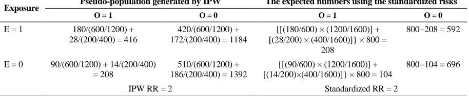
L is neither confounder nor effect modifier Table 1 shows the overall and L-specific joint distribution of E and O in a hypothetical population, in which both L and E affect O, but E and L are independent and thus L is not a confounder for the effect of E on O. Both L-specific RRs estimates in tables 1 are 2 implying no effect modification by L on the RR scale. The Mantel–Haenszel and maximum-likelihood L-adjusted RRs (using either binomial or log-Poisson regression) are 2, which are the same as crude RR. The marginal RR by both IPW and standardization equals the crude RR (2) reinforcing “no confounding”. The details of calculations of IPW and standardized RRs are described in Appendix 1.
L is confounder but not effect modifier
Table 2 presents the overall and L-specific joint distribution of E and O in a hypothetical population, in which both L and E affect O, and E and L are associated and thus L is a confounder for the effect of E on O. Although the crude RR in table 2 is 2.75, both L-specific
RRs are 2 implying no effect modification by L on the RR scale and considerable positive
confounding based on change-in-estimate
criterion. As expected, the Mantel–Haenszel and maximum-likelihood L-adjusted RRs (using either a log-binomial or log-Poisson regression) are 2. The marginal RR by both IPW and standardization is 2 which does not equal the crude RR (2.75) implying “confounding.”
L is effect modifier but not confounder
Table 3 shows the overall and L-specific joint distribution of E and O in a hypothetical population in which both L and E affect O, but E and L are independent and thus L is not a confounder for the effect of E on O. Based on table 3, the stratum- specific RRs are 4 and 2, implying substantial effect modification by L on the RR scale. The crude RR is 3.62 which equals
the marginal RR by both IPW and
standardization implying “no confounding,” In the absence of confounding, the crude RR value of 3.62 is the average of the L-specific RRs and is much closer to the value in the stratum L = 1
Table 1. No confounding without effect modification
Exposure L = 1 L = 0 Crude
O = 1 O = 0 Total O = 1 O = 0 Total O = 1 O = 0 Total
E = 1 180 420 600 28 172 200 208 592 800
E = 0 90 510 600 14 186 200 104 696 800
Total 1200 400 1600
RR = 2 RR = 2 RR = 2
IPW RR* = 2, Standardized RR* = 2, Mantel–Haenszel RR = 2, Maximum-likelihood L-adjusted RR (using either log-binomial or log-Poisson regression) = 2. *The details of calculation are presented in appendix 1. IPW: Inverse-probability-weighting, RR: Risk ratio
Table 2. Confounding without effect modification
Exposure L = 1 L = 0 Crude
O = 1 O = 0 Total O = 1 O = 0 Total O = 1 O = 0 Total
E = 1 324 756 1080 28 172 200 352 928 1280
E = 0 18 102 120 14 186 200 32 288 320
Total 1200 400 1600
RR = 2 RR = 2 RR = 2.75
IPW RR = 2, Standardized RR = 2, Mantel-Haenszel RR = 2, Maximum-likelihood L-adjusted RR (using either log-binomial or log-Poisson regression) = 2, IPW: Inverse-probability-weighting, RR: Risk ratio
Table 3. No confounding with effect modification
Exposure L = 1 L = 0 Crude
O = 1 O = 0 Total O = 1 O = 0 Total O = 1 O = 0 Total
E = 1 240 360 600 28 172 200 268 532 800
E = 0 60 540 600 14 186 200 74 726 800
Total 1200 400 1600
RR = 4 RR = 2 RR = 3.62
(i.e., 4), which contains substantially more of the population and it is thus weighted more in the
averaging (5). The Mantel–Haenszel and
maximum-likelihood L-adjusted RRs using a misspecified log-Poisson regression model (i.e., without product term between E and L) are 3.62; a misspecified log-binomial regression model yields a maximum-likelihood RR of 3.66, however.
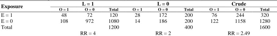
L is both confounder and effect modifier Table 4 presents the overall and L-specific joint distribution of E and O in a hypothetical population in which both L and E affect O, and E and L are associated and thus L is a confounder for effect of E on O. On the other hand, the stratum-specific RRs are 4 and 2, implying substantial effect modification by L on the RR scale. Thus, table 4 represents a scenario in which L is both confounder and effect modifier (on the RR scale). The Mantel– Haenszel and maximum-likelihood L-adjusted RRs using misspecified binomial and log-Poisson regression models (i.e., without product term between E and L) are 3.21, 3.58, and 3.47, respectively; because of effect modification, none of these values have exact causal interpretations, however. The marginal RR by both IPW and standardization is 3.62 which do not equal the crude RR of 2.49 implying “confounding”. Because of confounding, the crude RR value of 2.49 is much closer to the value in the stratum L = 0 (i.e., 2), even though it contains substantially less of the population. The Stata codes for all analyses in this section are provided in Appendix 2.
Discussion
We have illustrated the estimation of causal effects of a binary exposure on a binary outcome
in the presence of confounding and/or effect modification by a third binary variable, which is a risk factor for outcome. If the third variable is confounder but not effect modifier, the marginal and conditional RRs coincide, but they diverge from the crude RR. If the third variable is effect modifier but not a confounder, the marginal and crude RRs coincide, but they diverge from the different stratum-specific RRs. The difficulty arises when the third variable is both confounder and effect modifier, and subsequently neither crude RR nor the adjusted RR using a misspecified regression model (which assumes
no effect modification) has causal
interpretations. Therefore, the stratum-specific RR estimates are often reported in the presence of interaction between exposure and confounder(s) in the literature, even if the target of the intervention on the exposure is the total population and the interaction itself is not of interest. The reason is that researchers and practitioners are less familiar with marginal methods of adjustment such as IPW and standardization and marginal causal effects which have marginal causal interpretations for the total population even in the presence of interaction. Our results generalize to other collapsible effect measures such as risk difference and survival-time ratio, but not to non-collapsible measures such as odds ratio (OR) and rate ratio (6, 7). Under scenario 1, L is associated with O given E, because it affects O, and it is also associated with E given O, because both E and L affects O (i.e., O is a collider on the L→O←E in the causal diagram generating the data) (3, 8). Thus, assuming no effect modification on OR scale, the crude OR will not be equal to L-specific ORs i.e., OR is not (simply) collapsible over L, even though it equals the marginal causal OR derived by standardization or IPW and thus has a causal interpretation for the total population. This “OR non-collapsibility without confounding” can
Table 4. Confounding with effect modification
Exposure L = 1 L = 0 Crude
O = 1 O = 0 Total O = 1 O = 0 Total O = 1 O = 0 Total
E = 1 48 72 120 28 172 200 76 244 320
E = 0 108 972 1080 14 186 200 122 1158 1280
Total 1200 400 1600
RR = 4 RR = 2 RR = 2.49
happen in practice in certain designs (e.g., matched cohort studies), and regression models (e.g., random cluster-effects models) (6, 9). Assuming OR homogeneity, a converse property of “OR collapsibility without confounding” can occur under scenario 2 where L is a confounder, but it requires an exact cancellation, which is unlikely to occur in practice (10). In this rather theoretical case, the crude OR will be equal to the causal L-specific ORs even though it does not equal the marginal causal OR derived by standardization or IPW and thus does not have a causal interpretation for the total population.
The IPW and standardized RRs coincide in our simple data examples where there is only one binary covariate, and marginal RRs are non-parametrically estimated. However, there are often several nuisance covariates, some of them may be continuous or time-varying which necessities using regression models to estimate IPW and standardized effect estimates. Then, the results of standardization and IPW generally differ, because they rely on different modeling assumptions (IPW models the exposure on the confounders and standardization models the outcome on exposure and confounders) and some models misspecification is inevitable (3).
The intervention level of the exposure should be considered for causal effect estimation, especially in the presence of variables which are both confounders and effect modifiers. If the intervention is individual-level (e.g., drug use), the conditional stratum-specific effect estimates should be reported. However, if the level of intervention is population, the marginal effects are of interest and should be estimated and reported. The intervention level for many exposures including environmental exposures (e.g., air pollution) is population. Furthermore, the marginal effects with respect to time-dependent confounders affected by prior exposure should be estimated irrespective of the exposure level of intervention (11-13). Marginal causal methods are also helpful for estimating the population intervention parameters which are very relevant to public health policy (14). The researchers should bear in mind that differences between marginal and conditional causal effects may occur due to: (i) Misspecifying the
conditional model due to ignoring the effect modification(s) by the conditioning covariate(s) as illustrated in the last scenario where L is both confounder and effect modifier, (ii) non-collapsibility of certain effect measures as mentioned above in the case of OR for scenario 1 where L is neither confounder nor effect modifier; it is just a risk factor for outcome, and (iii) biases caused by conditioning on a time-dependent confounder affected by exposure (13, 15).
In practice, researchers often estimates a homogenous causal effect using an outcome regression model without assuming interaction between the exposure and several covariates, an assumption that is unlikely to be met in practice. Under common conditions, RR or risk difference estimates obtained from linear or log-linear probability models can be interpreted as approximate estimates of standardized RR, using the total source population as the standard (16, 17). However, this result does not apply to OR obtained from logistic regression models (unless risk is low at all exposure-covariates combinations), and rate ratio obtained from log-linear rate regression models (unless the exposure has very small effect on follow-up person-time) (6, 7, 17).
Acknowledgments
The authors gratefully acknowledge the financial support for this work provided by Tehran University of Medical Sciences, Tehran, Iran.
References
1. Greenland S, Rothman KJ . Introduction to
stratified analysis. In: Rothman KJ,
Greenland S, Lash TL, Editors. Modern epidemiology. Philadelphia, PA: Lippincott Williams & Wilkins; 2008. p. 258-82.
2. Greenland S, Lash TL, Rothman KJ.
Concepts of interaction. In: Rothman KJ, Greenland S, Lash TL, Editors. Modern epidemiology. Philadelphia, PA: Lippincott Williams & Wilkins; 2008. p. 71-83.
3. Hernan MA, Robins JM. Causal inference.
London, UK: Chapman and Hall; 2015.
4. Greenland S, Mansournia MA. Limitations
and ignorability assumptions, as illustrated
by random confounding and design
unfaithfulness. Eur J Epidemiol 2015.
5. Jewell NP. Statistics for epidemiology.
London, UK: Taylor & Franci; 2003.
6. Greenland S, Pearl J, Robins JM.
Confounding and collapsibility in causal inference. Statist Sci 1999; 14(1): 29-46.
7. Greenland S. Absence of confounding does
not correspond to collapsibility of the rate ratio or rate difference. Epidemiology 1996; 7(5): 498-501.
8. Glymour MM, Greenland S. Causal
diagrams. In: Rothman KJ, Greenland S, Lash TL, Editors. Modern epidemiology. Philadelphia, PA: Lippincott Williams & Wilkins; 2008. p. 183-209.
9. Mansournia MA, Hernan MA, Greenland S.
Matched designs and causal diagrams. Int J Epidemiol 2013; 42(3): 860-9.
10. Mansournia MA, Greenland S. The relation
of collapsibility and confounding to
faithfulness and stability. Epidemiology 2015; 26(4): 466-72.
11. Robins JM, Hernan MA, Brumback B.
Marginal structural models and causal inference in epidemiology. Epidemiology 2000; 11(5): 550-60.
12. Hernan MA, Brumback B, Robins JM.
Marginal structural models to estimate the causal effect of zidovudine on the survival of HIV-positive men. Epidemiology 2000; 11(5): 561-70.
13. Mansournia MA, Danaei G, Forouzanfar
MH, Mahmoodi M, Jamali M, Mansournia N, et al. Effect of physical activity on functional performance and knee pain in patients with osteoarthritis : analysis with marginal structural models. Epidemiology 2012; 23(4): 631-40.
14. Hubbard AE, Laan MJ. Population
intervention models in causal inference. Biometrika 2008; 95(1): 35-47.
15. Vansteelandt S, Keiding N. Invited
commentary: G-Computation–lost in
translation? Am J Epidemiol 2011; 173(7): 739-42.
16. Greenland S, Maldonado G. The
interpretation of multiplicative-model
parameters as standardized parameters. Stat Med 1994; 13(10): 989-99.
17. Greenland S. Introduction to regression
modeling. In: Rothman KJ, Greenland S, Lash TL, Editors. Modern epidemiology.
Philadelphia, PA: Lippincott Williams &
Appendix
Appendix 1: Calculation of IPW and standardized RRs
For calculating marginal RR with IPW method, we created a pseudo-population using
inverse-probability-of-exposure weighting. As an
example, 180 exposed outcome-positive
individuals in stratum L = 1 of table 1 were weighted with the inverse-probability of being exposed in L = 1 (i.e., 600/1200), and 28 exposed outcome-positive individuals in stratum L = 0 were weighted with the inverse probability of being exposed in L = 0 (i.e., 200/400), and then they were summed to produce the total number of exposed outcome-positive individuals in the
pseudo-population [i.e., 180/(600/1200) +
28/(200/400) = 416] presented in appendix table 1. Similar calculations were done to produce the other cells of the pseudo-population in appendix table 1. The IPW RR is the crude RR in the pseudo-population which is 2.
In the standardization method with total population as the standard, the exposure-specific risks were weighted-averaged across strata of L with weights equal to the proportion of individuals in each stratum of L. For example, the standardized risk in the exposed in table 1 is the weighted average of the risks in the exposed individuals in strata L = 1 and L = 0 with weights
1200/600 and 400/600, respectively i.e.,
[(180/600) × (1200/1600)] + [(28/200) × (400/1600)] = 0.26. Similarly, the standardized risk in the unexposed is [(90/600) × (1200/1600)] + [(14/200) × (400/1600)] = 0.13. Thus, the standardized RR is 0.26/0.13. The expected numbers of persons with and without outcome using the standardized risks are shown in appendix table 1.
Appendix 2: Stata code for analyses of the data in table 4
i.Constructing the data in table 4
input l e o freq 1 1 1 48 1 1 0 72 1 0 1 108 1 0 0 972 0 1 1 28 0 1 0 172 0 0 1 14 0 0 0 186 End
i. Obtaining Mantel–Haenszel and
maximum-likelihood L-adjusted RRs from log-binomial and log-Poisson regression
cs o e [fweight = freq], by(l)
glm o i.e i.l [fweight = freq], family(binomial 1) link(log) eform
glm o i.e i.l [fweight = freq], family(poisson) link(log) eform
ii. Obtaining IPW RR
expand freq quietly: logit e l predict pr, p gen w = 1/pr
replace w = 1/(1-pr) if e==0
glm o e [pweight = w], family(binomial 1) link(log) eform
iii. Obtaining standardized RR
Method 1
glm o i.e##i.l, family(binomial 1) link(log) eform
margins e
Table 1. Calculation of IPW and standardized RR for data presented in table 1
Exposure Pseudo-population generated by IPW The expected numbers using the standardized risks
O = 1 O = 0 O = 1 O = 0
E = 1 180/(600/1200) +
28/(200/400) = 416
420/(600/1200) + 172/(200/400) = 1184
{[(180/600) × (1200/1600)] + [(28/200) × (400/1600)]} × 800 =
208
800−208 = 592
E = 0 90/(600/1200) + 14/(200/400) = 208
510/(600/1200) + 186/(200/400) = 1392
{[(90/600) × (1200/1600)] + [(14/200)×(400/1600)]} × 800 = 104
800−104 = 696
IPW RR = 2 Standardized RR = 2
matrix b = r(b) di b[1,2]/b[1,1] Method 2 gen id = _n
expand 2, gen(counterfactual)
label define counterfactual 0 “actual” 1 “counterfactual”
replace e = 1- e if counterfactual==1
quietly: logit o i.e.##i.l if counterfactual==0 predict p, p
reshape wide p counterfactual, i(id) j( e) sum p1
scalar r1 = r(mean) sum p0