A GENERAL BOUNDARY ELEMENT FORMULATION FOR
THE ANALYSIS OF VISCOELASTIC PROBLEMS
H. Ashrafi*and M. Farid
Center of Excellent in Computational Mechanics, Department of Mechanical Engineering, School of Engineering, Shiraz University, Shiraz 71348, Iran
[email protected] , [email protected]
*Corresponding Author
(Received: April 24, 2009 – Accepted in Revised Form: May 20, 2010)
Abstract The analysis of viscoelastic materials is one of the most important subjects in engineering structures. Several works have been so far made for the integral equation methods to viscoelastic problems. From the basic assumptions of viscoelastic constitutive equations and weighted residual techniques, a simple but effective Boundary Element (BE) formulation is developed for the Kelvin viscoelastic solid models. This formulation needs only Kelvin’s fundamental solution of isotropic elastostatics with material constants prescribed as explicit functions of time. It is able to solve the quasistatic problems with any load dependence and boundary conditions. A system of time-dependent equations is derived by imposing the convenient approximations and adopting the kinematical relations for strain rates. This approach avoids the use of relaxation functions and mathematical transformations. The main feature of the proposed formulation is the absence of domain discretizations, which simplifies the treatment of problems involving infinite domains. A computer code has been developed in the programming environment of MATLAB software. At the end of this paper, two numerical examples have been provided to validate this formulation.
Keywords Viscoelastic Solids, Boundary Element Approach, Kelvin Solid Model
ﻩﺪﻴﻜﭼ
ﻩﺯﺎﺳ ﺭﺩ ﺕﺎﻋﻮﺿﻮﻣ ﻦﻳﺮﺘﻤﻬﻣ ﺯﺍ ﯽﮑﻳ ﮏﻴﺘﺳﻻﺍﻮﮑﺴﻳﻭ ﻞﺋﺎﺴﻣ ﻞﻴﻠﺤﺗ ﯽﻣ ﯽﺳﺪﻨﻬﻣ ﯼﺎﻫ
ﺪﺷﺎﺑ . ﺵﻼﺗ ﯽﻳﺎﻫ
ﺖﻓﺎﻴﻫﺭ ﺎﺑ ﮏﻴﺘﺳﻻﺍﻮﮑﺴﻳﻭ ﻞﺋﺎﺴﻣ ﻞﺣ ﺭﻮﻈﻨﻣ ﻪﺑ ﻥﻮﻨﮐﺎﺗ ﯼﺎﻫ
ﻒﻠﺘﺨﻣ ﺖﺳﺍ ﻪﺘﻓﺮﮔ ﻡﺎﺠﻧﺍ ﯽﻟﺍﺮﮕﺘﻧﺍ ﺕﻻﺩﺎﻌﻣ .
ﻦﻳﺍ ﺭﺩ
،ﻪﻟﺎﻘﻣ ﻝﻮﻣﺮﻓ ﮏﻳ ﻥﺎﻤﻟﺍ ﯼﺪﻨﺑ
ﻔﺘﺳﺍ ﺎﺑ ﺮﺛﺆﻣ ﺭﺎﻴﺴﺑ ﯽﻟﻭ ﻩﺩﺎﺳ ﯼﺯﺮﻣ ﯼﺎﻫ ﻴﺿﺮﻓ ﺯﺍ ﻩﺩﺎ
ﻪ ﯼﺎﻫ ﻦﻳﺩﺎﻴﻨﺑ ﻪﻠﮑـﺸﺘﻣ ﺕﻻﺩﺎـﻌﻣ
ﻝﺪﻣ ﯼﺍﺮﺑ ﯽﻧﺯﻭ ﺪﻧﺎﻤﺴﭘ ﻝﻮﺻﺍ ﻭ ﮏﻴﺘﺳﻻﺍﻮﮑﺴﻳﻭ
ﺖـﺳﺍ ﻪـﺘﻓﺎﻳ ﻪﻌـﺳﻮﺗ ﯽﻨﻳﻮـﻠﮐ ﺪـﻣﺎﺟ ﮏﻴﺘﺳﻻﺍﻮﮑﺴﻳﻭ ﯼﺎﻫ .
ﻦـﻳﺍ
ﻝﻮﻣﺮﻓ ﻪـﮐ ﺩﺭﺍﺩ ﺯﺎﻴﻧ ﮏﻴﭘﻭﺮﺗﻭﺰﻳﺍ ﮏﻴﺗﺎﺘﺳﺍﻮﺘﺳﻻﺍ ﻞﺋﺎﺴﻣ ﺭﺩ ﻩﺩﺎﻔﺘﺳﺍ ﺩﺭﻮﻣ ﻦﻳﻮﻠﮐ ﯽﺳﺎﺳﺍ ﺏﺍﻮﺟ ﻪﺑ ﺎﻬﻨﺗ ﺪﻳﺪﺟ ﯼﺪﻨﺑ
ﺕﺭﻮﺻ ﻪﺑ ﻥﺁ ﺭﺩ ﯼﺩﺎﻣ ﺖﺑﺍﻮﺛ ﻩﺪﺷ ﻒﻴﺻﻮﺗ ﻥﺎﻣﺯ ﺯﺍ ﯽﺤﻳﺮﺻ ﻊﺑﺍﻮﺗ
ﺪﻧﺍ . ﻪـﺑ ﻪﺘـﺴﺑﺍﻭ ﯼﺎﻫﺭﺎﺑ ﻉﻮﻧ ﺮﻫ ﻝﺎﻤﻋﺍ ﺖﻴﻠﺑﺎﻗ
ﺩﺭﺍﺩ ﺩﻮﺟﻭ ﮏﻴﺗﺎﺘﺳﺍ ﻪﺒﺷ ﻞﺋﺎﺴﻣ ﻞﺣ ﯼﺍﺮﺑ ﺖﻓﺎﻴﻫﺭ ﻦﻳﺍ ﺭﺩ ﯼﺯﺮﻣ ﻂﻳﺍﺮﺷ ﻭ ﻥﺎﻣﺯ .
ﻪﻋﻮﻤﺠﻣ ﻪﺘـﺴﺑﺍﻭ ﺕﻻﺩﺎﻌﻣ ﺯﺍ ﯼﺍ
ﺶﻧﺮﮐ ﺥﺮﻧ ﯼﺍﺮﺑ ﯽﮑﻴﺗﺎﻤﻨﻴﺳ ﻂﺑﺍﻭﺭ ﻢﻴﻤﻌﺗ ﻭ ﺐﺳﺎﻨﻣ ﺕﺎﻴﺿﺮﻓ ﻝﺎﻤﻋﺍ ﺎﺑ ﻥﺎﻣﺯ ﻪﺑ
ﺖـﺳﺍ ﻩﺪـﺷ ﺝﺍﺮﺨﺘـﺳﺍ ﺎﻫ .
ﻦـﻳﺍ ﺭﺩ
ﻧ ﻩﺩﺎﻔﺘﺳﺍ ﻩﺪﻴﭽﻴﭘ ﯽﺿﺎﻳﺭ ﺕﻼﻳﺪﺒﺗ ﻭ ﯽﺷﺰﺧ ﺎﻳ ﯽﮔﺪﻴﻫﺭﺍﻭ ﻊﺑﺍﻮﺗ ﺯﺍ ﺖﻓﺎﻴﻫﺭ ﯽﻤ
ﺷ ﻮ ﺩ . ﻝﻮﻣﺮﻓ ﯽﮔﮋﻳﻭ ﻦﻳﺮﺘﻤﻬﻣ ﯼﺪـﻨﺑ
ﻪﺘﺴﺴﮔ ﻪﺑ ﺯﺎﻴﻧ ﻡﺪﻋ ﺭﺩ ﻩﺪﺷ ﻪﺋﺍﺭﺍ ﯼﺯﺎﺳ
ﻪﻨﻣﺍﺩ ﯼﺎﻫ ﺰـﻴﻧ ﺖـﻳﺎﻬﻨﻴﺑ ﻪـﻨﻣﺍﺩ ﺎﺑ ﻞﺋﺎﺴﻣ ﺭﺩ ﻩﺩﺎﻔﺘﺳﺍ ﯼﺍﺮﺑ ﺍﺭ ﻥﺁ ﻪﮐ ﺖﺳﺍ ﯼﺍ
ﺏﻮﻠﻄﻣ ﺖﺳﺍ ﻪﺘﺧﺎﺳ .
ﻧﺮﺑ ﻂﻴﺤﻣ ﺭﺩ ﯼﺮﺗﻮﻴﭙﻣﺎﮐ ﺪﮐ ﮏﻳ ﻪﻣﺎ
ﺐـﻠﺗﺎﻣ ﺭﺍﺰـﻓﺍ ﻡﺮـﻧ ﯽﺴﻳﻮﻧ )
MATLAB
( ﻪـﺘﻓﺎﻳ ﻪﻌـﺳﻮﺗ
ﺖﺳﺍ . ﻝﻮﻣﺮﻓ ﻦﻳﺍ ﯼﺯﺎﺳﺮﺒﺘﻌﻣ ﺭﻮﻈﻨﻣ ﻪﺑ ﯼﺩﺮﺑﺭﺎﮐ ﯼﺩﺪﻋ ﻝﺎﺜﻣ ﻭﺩ ﺪﻧﺍ ﻩﺪﺷ ﻪﺋﺍﺭﺍ ﻪﻟﺎﻘﻣ ﻥﺎﻳﺎﭘ ﺭﺩ ﯼﺪﻨﺑ
.
1. INTRODUCTION
Because of the complexity of viscoelastic models which include time as an independent variable, the available exact analytical solutions have been obtained for only a few simplified problems. In the literature of computational solid mechanics, a large number of the computational methods to solve the various mechanical problems can be found. The
importantly, the problems that once seemed completely inflexible for an analytic study can be now analyzed by this technique rather easily. BEM has the advantage of requiring only boundary data as input and, no division of the domain under consideration into elements. In addition, the BEM is ideally suited for the analysis of infinite domains problems involving because only their surface has to be discretized and conditions at infinity are automatically satisfied by the Kelvin's fundamental solution.
The viscoelastic problems can be effectively treated by the BEM formulation. Numerous researchers developed the boundary element formulations to model the viscoelastic behavior. The first classical procedure for solving the viscoelastic problems is the use of mathematical transformations, in which, based on corresponding theorem [1-5], viscoelastic solutions are usually obtained by inverting the transformation of their associated elastic solutions. The viscoelastic equations can be transformed into equivalent elastic ones by means of Laplace transforms. After solving the transformed problem, a numerical inversion can be performed recovering the desired time domain behavior. Due to the complexity of the viscoelastic behavior, however, such treatment is feasible only in cases with simple geometry or idealized boundary conditions. In addition, this method is too complicated to use unless the relaxation or creep moduli can be accurately interpreted by a simple model. This procedure presents some difficulties when the viscous parameters are time varying, or when complicated time dependent boundary conditions are imposed. Another procedure is also available based on incremental scheme [6-10]. This kind of procedure uses the relaxation functions to transform the convolutional aspect of the viscous behavior in discrete contributions added to the elastic response. The other available formulation follows the same scheme applied to viscoplastic ones [11-13]. These techniques are based on the quasistatic incremental schemes where the time behavior of the solution is recovered by the stress decay, therefore, imposing the external loads with arbitrary time dependence presents some difficulties. In the following, several important works are investigated .
The usual approach, originally adopted by
Rizzo and Shippy [1], has been to formulate a BEM solution for the Laplace transforms of all variables satisfying an associated elastic problem, and then the solution in time domain is obtained by numerical inversion. Also, incremental BEM solutions in the time domain were first formulated by Shinokawa, et al [6]. Kusama and Mitsui [14] analyzed the linear viscoelastic problems using the boundary element method together with the numerical inversion of the Laplace transform. Their method reduced the amount of manual and computing time as compared with the finite element method.
The weighted residual technique, the indirect BEM, the truncated indirect BEM, and the direct BEM can be used to analyze nonlinear soil-structure interaction in time domain. They illustrated and compared by using 1-D dynamic problem of the spherical cavity in an infinite space by Wolf and Dorbe [15]. For realistic time steps, all formulations led to accurate results, but the weighted residual technique and the truncated indirect BEM were much more efficient than the direct BEM in time domain. Sim and Kwak [16] formulated isotropic, linear viscoelastic problems in time domain by BEM. The viscoelastic fundamental solutions were represented in terms of the constant coefficients of relaxation functions. From the reciprocal work theorem, an alternative form of boundary integral equations was derived by integration by parts. This form required the regularity of field variables to be one order less than that in the usual formulation. A time marching process was incorporated in the numerical method.
were given for 3D-continua, 2D-plane strain and the 2D-plane stress problems using the wide range of linear viscoelastic constitutive law models. An elaborate scheme, generating the time domain fundamental solution in a more general case, was developed by Lee, et al [19]. They proposed the method based on the Laplace transform and the correspondence principle. The relaxation function was expanded in a sum of exponentials, and the transformed fundamental solutions were inverted numerically into real time space.
Pan, et al [20] presented a BEM formulation for 3D linear and viscoelastic bodies subjected to the body force of gravity. First, Laplace transformation was used to suppress the time variable, and then the solutions of displacements and stresses were found in transformed domain. The time domain solutions were then found using an accurate and efficient numerical inversion method which required only real calculations for all quantities. The Green’s functions in Laplace domain were obtained through the correspondence principle.
Schanz [21] applied a quadrature rule for the convolution integrals, and/or the convolution quadrature method (CQM). With this numerical quadrature formula, he determined the integration weights from the Laplace transformed fundamental solution and a linear multi-step method. Finally, he obtained a BE formulation in time domain using all the advantages of the Laplace domain formulation. Even materials with complex Poisson’s ratio, leading to time-dependent integral free terms in the boundary integral equation, can be treated by this formulation. Mesquita and Coda [22 – 23] implemented Kelvin and Boltzmann viscoelastic models in a 2-D BE atmosphere. Their general methodology was based on differential constitutive relations for viscoelasticity. First part of their work described a methodology using the internal cells. This methodology makes it possible to consider viscous parameters, which are not proportional to elastic tensor. They obtained a simple time-marching process from the kinematical relations. In second part, the important algebraic operations were introduced into the formulation allowing analysis of the viscoelastic problems without internal cells.
Wang and Birgisson [24] presented a time domain BEM to model the quasistatic linear
viscoelastic behavior of asphalt pavements. In this viscoelastic analysis, the fundamental solution was derived in terms of the elemental displacement discontinuities (DDs) and a boundary integral equation was formulated in time domain. The unknown DDs were assumed to vary quadratically in the spatial domain and to vary linearly in time domain. The equations were then solved incrementally through the whole time history using an explicit time-marching approach. The spatial and time integrals were evaluated analytically, which gives highly accurate results and fast convergence of the numerical scheme. Recently, the researchers developed an alternative FEM formulation to analyze the viscoelastic problems based on the constitutive equations of the Kelvin and SLS models [25, 26]. Ashrafi and Farid [27] presented a general BEM formulation from the basic assumptions of SLS viscoelastic constitutive equations, in which it needs only the Kelvin’s fundamental solution of isotropic elastostatic problems. These formulations are based on the differential constitutive relation of the SLS viscoelastic model. They produced the time differential systems of equations, which can be solved by an appropriate time marching process.
provided to validate the proposed formulation.
2. VISCOELASTIC CONSTITUTIVE RELATIONS
Mathematically, the usefulness of constitutive equations is to describe the relationships among the kinematical, mechanical, and thermal field equations and to permit the formulations of well-posed problems in the continuum mechanics. Physically, constitutive equations define various idealized materials which serve as models for the behavior of real materials. All actual materials store and dissipate energy in varying degrees during a loading/unloading cycle [28]. A number of important engineering materials, such as solid polymers, simultaneously store and dissipate mechanical energy when subjected to the applied forces [29]. This form of response as a combination of both liquid-like and solid-like features is termed as viscoelasticity. Thus, the valid constitutive equations for the viscoelastic behavior incorporate elastic deformation and viscous flow as special cases, and at same time provide for the response patterns that characterize the combined behavior. Intrinsically, such constitutive equations will involve not only stress and strain, but time-rates of both stress and strain as well [28].
The behavior of viscoelastic materials in the uniaxial stress closely resembles that the models built from discrete elastic and viscous elements. Extensive experimental evidence has shown that practically all engineering materials behave elastically in dilatation; therefore without serious loss of generality, we may assume the fundamental constitutive equations for the linear viscoelastic behavior in differential operator form to be [28]:
ij ij Q
S
P} 2{ }
{
(1)
ii ii K
3 (2)
for isotropic media. Sij and ηij are the elements of
shear stress and strain tensor, respectively. The coefficients {P} and {Q} are differential time operators of the form:
N
i
i i i
t p P
0
(3)
M
i
i i i
t q Q
0
(4)
in which the coefficients pi and qi (not necessarily constants) represent the viscoelastic properties. Also, K is the bulk modulus. Note further that this pair of equations specifies separately the deviatoric and volumetric responses.
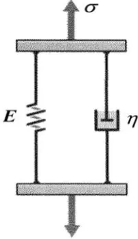
Based upon the two fundamental elements of elastic spring and viscous dashpot to model viscoelastic behavior, it is easy to construct the viscoelastic models by suitable combinations of this pair of elements. One especially simple combination that immediately comes to mind is the Kelvin or Voigt viscoelastic model. This model is a simple representation of this kind of behavior. The Kelvin solids consist of a spring and dashpot in parallel, as shown in Figure 1. For which, Equations 1 and 2 reduce to the following single equation [28]:
t
ij ij E (5)
where E and η represent the material constants (Figure 1), and the partial derivative with respect to time is denoted by ∂t. In general, from Figure 1,
the following relations can be expressed:
Figure 1. Sketch of the Kelvin model representing a
v ij e ij ij
(6)
v ij e ij ij
(7)
where the Cartesian coordinates are represented by subscripts i and j, while the superscript v and e
represent viscous and elastic parts, respectively. The stress-strain equations for the linear elastic solids assuming infinitesimal strains can be written as [28, 30]:
km ijkm e
ij C
(8)
where Cijkm are the elastic constants representing
the properties of the body, and can be defined as [30]:
ik jm im jk
km ij ijkm
C (9)
where λ and μ are Lame’s constants, given by:
) 2 1 ( ) 1
(
E
(10)
) 1 (
2
G E (11)
in which E and ν are Young’s modulus and Poisson ratio, respectively. In addition, δij is the
Kronecker delta.
Similarly, for the viscous stress components, following relations can be given:
mn ijmn v
mn ijmn v
ij K K
(12)
where the constant Kijmn represent viscous
properties of the body, and can be defined as [30]:
im jn in jm
mn ij ijmn
K
) ( ) (
(13)
in which and are the hydrostatic and
deviatoric viscosity coefficients, respectively
By substituting Equations 8 and 12 into Equation 6, we have:
kl ijkl kl ijkl
ij
C
K
(14)In this numerical formulation, in order to obtain only boundary integral equations, a simplification for the viscosity coefficients and
is assumed, i.e. . Therefore, Equation 14 changes into:
kl ijkl kl
ijkl
ij
C
C
(15)3. BOUNDARY ELEMENT FORMULATION
The boundary element method is based on boundary integral equations. There are several methods of deriving the boundary element formulations: the reciprocal theorem, the weighted residual concept and the variational approach. Here, the boundary integral equations, by extending to the Kelvin solid model, will be derived using the weighted residual concept.
The viscous effects should be included into the equilibrium equation of the body by relating numerically strain time rates with velocity in a way that the viscous characteristics of the body satisfy the boundary conditions together with the elastic ones. In order to do these requirements, the equilibrium equations for a general viscoelastic body can be written as:
j j j i
ij B u cu
, (16)
Or
j j j v
i ij e
i
ij B u cu
, , (17)
where Bj is the body force acting in j direction.
Since, in this work, the dynamic effects will not be considered, Equation 17 should be rewritten as:
0
,
, j
v i ij e
i
ij B
(18)
0
,j i ij B
(19)
In BEM, the Kelvin fundamental solution of an elastic infinite body is adopted as a proper function for weighting the differential equilibrium relation [31-32]. Therefore, Equation 19 can be weighted over the considered domain D as:
dv
0
, Dki ijj Bi (20)
where
ψ
ki is the Kelvin fundamental solution. Itrepresents the effect of a unit concentrated load applied at a point located in an infinite domain. Integrating Equation 20 by parts and then applying the divergence theorem yields:
D ki i D kij ij
D ki ij j
dv B dv s d n , 0 (21)
where ∂D is the boundary of the body and nj is the
outward normal vector component. By knowing that,
n i j ijn t
(22) and ij j ki ij j ki i kj ij i kj j ki ij kij , , , , , ) ( 5 . 0 ) ( 5 . 0 (23)
where
kij is the strain fundamental term, Equation
21 changes into:
D ki i D kij ij
D n i ki dv B dv s d t 0 (24)
The next equation is the starting point to derive the viscoelastic integral equations. By imposing the viscoelastic relations, i.e. Equation 15, into Equation 24, we have:
D ki i D kij ijmn mn
D kij ijmn mn D n i ki dv B dv C dv C s d t ) ( ) ( 0 (25)
Also, by knowing that,
j i kij n m kmn mn kmn mn ijmn kij u u C , , (26) And j i kij n m kmn mn kmn mn ijmn kij u u C , , (27)
Equation 25 changes into:
D ki i D kij ij
D kij ij D n i ki dv B dv u dv u s d t , , 0 (28)
By using integrating by parts of the second and third terms of Equation 28, we have:
D ki i D kijj i
D kij j i D kijj i
D kij j i D n i ki dv B dv u ds u n dv u ds u n s d t , , 0 (29)
Equation 29 can be rewritten by using the fundamental equilibrium equation, i.e.
ki jkij x y
,
, (30)
where δ(x, y) is the Dirac’s delta distribution, in which y is a field point and x is the source point. By knowing that,
n
ki j
kijn t (31)
Equation 29 changes into:
D ki i
D i n ki D i n ki D n i ki i ki i ki dv B ds u t ds u t s d t x u C x u C ( ) ) ( (32)
where the free term Єji is exactly what was
the integral equation for the general Kelvin–Voigt viscoelastic solids.
The body force domain integral can be easily transformed into its boundary integral equation, which results an equation written exclusively for boundary values. The simple and robust method, which is called the radial integration method, was used for transforming the domain integrals into the equivalent boundary integrals [33]. Any 2-D or 3-D domain integral can be evaluated in a unified way without need to discretize the domain into internal elements. By assuming that the body force Bi is constant, the
domain explicit integral equation is converted to the boundary integral equation. Therefore, we have: ds B B ds n r r dr r B d dr r B dv B dv B D ki i D r ki
i
r ki i
D ki i D ki i
1 (33)in which,
ki
B , for the Kelvin fundamental solution, is given by:
n r r r r G r B i k ki ki , , 2 1 ln ) 3 4 ( ) 1 ( 16 (34)
By applying above changes into Equation 32, results:
D ki i D i n ki D i n ki D ki i ki i ki ds B B ds u t ds u t s d x u C x u C ( ) ) ( (35)Finally, it is worth to note that the necessary kernels ki and n
ki
t , for the 2-D elastostatic problems can be obtained in BE handbooks with the either plane strain or plane stress conditions [31-32]. In a similar way to displacement integral equations, the boundary stress integral equations can be derived to calculate the stress fields on the boundary.
3.2. Stress Integral Equations
To derive the stress integral equation for interior points, one starts by deriving the strain integral equation. At interior points, the displacement integral equation is given by:
D ki i D i n ki D i n ki D n i ki k k ds B B ds u t ds u t s d t x u x u ( ) ) ( (36)Denoting the displacements ui and the displacement rates ui in tensor notation, the both
small strains and small strain rates are related to displacements and displacement rates via [34]:
kl lk
kl
u
,u
,2
1
(37)
kl lk
kl
u
,u
,2
1
(38)By substituting the above relations in Equation 36 and by considering that the derivatives are done with respect to the source point location, we find:
D kil i D i n kil D i n kil D n i kil kl klds
B
B
ds
u
t
ds
u
t
s
d
t
x
x
~
~
~
)
(
)
(
(39)The total stress is obtained using the constitutive Equation 15 in Equation 39, resulting in:
D i D i n D i n D n i v mn e mnds
B
B
ds
u
t
ds
u
t
s
d
t
x
x
min min min min)
(
)
(
(40)Now, the total stress state is obtained using the general constitutive Equation 6 and Equation 40:
D i D i n D i n D n i mnds
B
B
ds
u
t
ds
u
t
s
d
t
x
min min min min)
(
(41)where
ijk,
n ijk
t ,
ijk
B and
can be defined by following relations (by using [31]):
ij k jk i ik j i j k
ijk r r r r r r r , , , , , , 2 3 ) ( ) 2 1 ( 1 ) 1 ( 8 1 (42)
ij k jk i ik j j i k k i j k j i k j i i kj j ik k ij n ijk n n n r r n r r n r r n r r r r r r n r r E t ) 4 1 ( 3 ) 2 1 ( ) ( 3 5 ) ( ) 2 1 ( 3 1 ) 1 ( 8 , , , , , , , , , , , , 3 2 (43) n r Bijk ijk (44) and
ij k jk i ik j k i j
ijk r r r r r r r E y x , , , , ,
, ) 2
( ) 4 3 ( 1 ) 1 ( 4 1 ) , ( (45)
In order to determine the elastic and viscous stress states of total stress fields, from Equation 41, Equation 8 can be written in following form:
vij km ijkm km ijkm e
ij C C
1 1 (46)
By substituting the above relation into the equilibrium equation, a time-dependent equation can be derived as:
0 e ij e ij ij
(47)
Finally, we can solve numerically Equation 47 by an adaptive linear approximation for the elastic stress field.
4. NUMERICAL DISCRETIZATION
It is only possible to solve boundary element formulation (i.e. Equations 35 and 41) analytically
for very simple problems. The first step in the discretization is to divide the boundary ∂D into Ne elements, so that Equations 35 and 41 become:
e r e r e r e r N r D ki i N r D i n ki N r D i n ki N r D n i ki i ki i ki ds B B ds u t ds u t s d t x u C x u C 1 1 1 1 ) ( ) ( (48) and
e r e r e r e r N r D i N r D i n N r D i n N r D n i mn ds B B ds u t ds u t s d t x 1 min 1 min 1 min 1 min ) ( (49)where ∂D = ∑∂Dn.
5. ISOPARAMETRIC ELEMENTS
One of the most significant improvements in the BEM was the introduction of the parametric representation of both geometry and unknown functions similar to isoparametric formulation in the FEM. In this type of formulation, the boundary parameter yi, the unknown displacement and
velocity fields ui and ůi, and also the traction fields
ti are approximated by introducing interpolation functions in following forms, respectively:
where, Nα called shape functions, are polynomials
of degree m-1. The quantities yi, ui , ui and
n i
t are the values of the functions at node
. These shape functions are defined in terms of non-dimensional coordinates ξ (-1 ≤ ξ ≤ 1). Here, for discretization of the boundary, the linear elements (m = 2) have been used; therefore for these elements, we have:
1 1 2 1 2 2 1 1 N N (51)A discretized boundary element formulation can be obtained by substituting the relations of Equation 50 into the chief integral Equations 48 and 49, to obtain:
e r e r e r e r N r D ki i N r m D r i n ki N r m D r i n ki N r m D nr i ki i ki i ki ds B B ds u N t ds u N t s d t N x u C x u C 1 1 1 1 1 1 1 ) ( ) ( (52) and
e r e r e r e r N r i DN r m D r i n N r m D r i n N r m D nr i mn ds B B ds u N t ds u N t s d t N x 1 min 1 1 min
1 1 min
1 1 min ) ( (53)
Due to the similar shape functions used for approximation of the geometry and functions, the formulation is referred to as isoparametric. After choosing the same number for the source points and nodes and then calculating all integrals, the
discretized boundary element equations may now be written in the matrix form as:
) B( D ) t( G ) ( u H ) u(
H t β t t t (54)
and ) ( u H ) u( H ) B( D ) t( G )
σ(t t t t β t (55)
where t represents the time.
6. NUMERICAL ALGORITHM
To solve the time-dependent differential matrix Equations 54 and 55, it can be necessary to approximate velocity in time domain by a proper time marching treatment. This is carried out by choosing a linear behavior along the time, as follows: t s s s u u u 1 1 (56)
The following linear time marching process, by substituting Equation 56 into Equation 54, has been derived:
s 1 s 1
s Gt F
u
H
(57) in which H H t 1 (58) and 1 s s
s Hu DB
F
t
(59)
As previous values are known, now it is necessary to solve the matrix system of Equation 57 for the current time (tn+1). In addition, the
matrices. un+1 and tn+1 can be obtained from Equation 57.
For calculating the total stress state, Equation 55 for the current time (tn+1) can be
computed as:
1
1
s1 s1 s1 s
s Gt DB Hu βHu
σ (60)
in which us1 is derived from Equation 56. By assuming the linear behavior along the time domain for the elastic stress rates as:
t
e s e
1 s e
1 s
σ σ
σ (61)
and by substituting it into Equation 47, we have:
s1 es
e 1 s
1 1
σ σ
σ
t t
(62)
Elastic stress state can be obtained from Equation 62, in which e
s
σ is known and σs1 is derived by Equation 60. The presented algorithm has been cast into a unique program and has been solved using the commercial software MATLAB. A computer code "VBE_KEL" was developed into MATLAB.
7. NUMERICAL EXAMPLES AND RESULTS
For validating accuracy of presented formulation, it has been used to solve the two numerical viscoelastic problems shown below whose results can be compared with the analytical solutions.
7.1. Example One; Pressurization of a
Viscoelastic Compressible Cylindrical Tank
The problem of the pressurization of a viscoelastic cylinder is of technical important [2-4]. The considerations here are for sufficiently long cylinders such that plane strain conditions can be assumed.
A thick-walled cylindrical tank, as shown in Figure 2, under radial internal pressure Pi is
analyzed. In the plane of the cross section, we use a polar coordinate system r, θ and normal to them
z axis. Continuity of the deformation in plane strain demands that εz = 0. Theory of elasticity
yields the following formulas for the radial stress
σr, the tangential stress σθ and the radial
displacement u subjected to internal pressure Pi:
2
r B A
r
(63)
2
r B A
(64)
Figure 2. The cylindrical tank under the radial internal
pressure (P).
Figure 3. BE Discretization of the model under the radial
and
r B r A
E r
u( ) 1 1 2 (65)
in which constants A and B are determined from boundary conditions. For this problem, the boundary conditions are:
0
2 1
r i r
R r
p R
r
(66)
Upon inserting above conditions:
2 1 2 2
2 2 2 1 2
1 2 2
2 1
R R
R R p B R R
R p
A i i
(67)
where R1 and R2 are the inside and outside radii of tank, respectively.
As shown by Equations 63 and 64, the stresses in elastic body are independent of the material constants. Therefore, in accordance with the elastic-viscoelastic correspondence principle, the stresses will be the same when the cylinder is made of a viscoelastic material. Since the displacement u
is a function of material constants, it will be time dependent. The time dependence may be found by employing the corresponding principle [2-4]. With considering cylinder as a Kelvin viscoelastic solid and applying correspondence principle, the actual radial displacement is obtained:
A q
t q r
q R
q t q K q
K r t
r u
1 0
0 2 2
1 0
0
exp 1
) 6 ( exp 1 6
3 )
, (
(68)
in which K is the bulk modulus, and q0 and q1 are the coefficients of the Kelvin solids. The analytical and numerical results for displacements have been calculated for the following parameters:
) )( ( 10 2
) ( 10 2
10 9
6 1
5 5 0
Days MPa q
MPa K
q
(69)
TABLE 1. Parameters of the First Modeling.
Mechanical
Properties E = 20 (MPa) υ = 0.4 β(days) = 14
Geometry R1 = 10 (in)
= 250 (mm) R2 = 2 (R1)
---Time
Increment Δt = 1 (day) ---
---Pressurization P = 2000 (KPa) ---
---Due to double symmetry of the problem, only a quarter of problem is modeled, as shown in Figure 3. The geometry and mechanical properties of the model are shown in Table 1.
The numerical solution is obtained by using 30 elements and using 20 steps in time- – marching process to arrive at t = 120 days. The inner and outer wall radial displacement obtained using this numerical formulation is compared with the analytical ones as shown in Figure 4 and Figure 5, respectively. The radial displacement at interior point (A: [0.53 R2, 0.53 R2]) obtained by this numerical formulation has also been compared with the analytical one as shown in Figure 6. It can be observed that the agreement of the obtained results of this formulation with those of analytic ones is very good.
0 20 40 60 80 100 120
0 5 10 15 20 25 30 35 40 45 50
55 Inner Wall
Time (days)
D
is
p
la
ce
m
en
t (m
m
)
Analytic Solution Numerical Solution Elastic Solution
Figure 4. The radial inner wall displacement as compare to
0 20 40 60 80 100 120 0
5 10 15 20 25 30
35 Outer Wall
Time (days)
D
ispl
acem
en
t (
m
m
)
Analytic Solution Numerical Solution Elastic Solution
Figure 5. The radial outer wall displacement as compared to
the analytical solution.
0 20 40 60 80 100 120
0 5 10 15 20 25 30 35
40 Interior Point A
Time (days)
D
ispl
acem
ent
(m
m
)
Analytic Solution Numerical Solution Elastic Solution
Figure 6. The radial displacement at interior point (A) as
compared to the analytical solution.
0 20 40 60 80 100 120
0 10 20 30 40 50
60 Time Step Length Dependence
Time (days)
D
is
p
la
ce
me
n
t (
mm)
dt=0.01 dt=0.1 dt=1 dt=5 dt=10
Figure 7. Dependence effect to the time step length of the
radial inner wall displacement as compared to the corresponding analytical solution.
Time step dependence for the proposed formulation is also shown in Figure 7 for the inner wall radial displacement. As it can be observed, the obtained results are rather accurate even for the large time steps. However, the final elastostatic solution is achieved for any chosen time step.
It is worth noting that this formulation can easily be used for plane stress conditions by changing in material constants. A hole or a crack in an infinite viscoelastic structure can be modeled as a Kelvin solid and is then analyzed by this formulation for plane stress conditions.
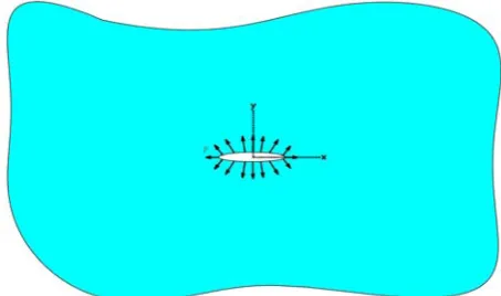
7.2. Example Two; A Pressurized Crack in
an Infinite Viscoelastic Plane Structure
As another example, we consider the problem of a pressurized crack in a viscoelastic plane structure made of the Kelvin model. For simplicity, the crack is assumed to be aligned along the x axis with the center located at the origin of the coordinate system as shown in Figure 8. The length of the crack is 2a and the crack surfaces have been subjected to the uniform normal pressure P.The analytical solution for the crack opening displacement for the elastic structure cases is given as [35]:
P x a G x
u( ) 2(1 ) 2 2
(70)
where G and ν are the elastic constants and also ∆u
denotes the crack opening displacement.
Since the crack opening displacement is a function of the material constants, it will be time dependent. The time dependence may be found by employing the corresponding principle [2-4]. The viscoelastic solution, using the correspondence principle and the analytical Laplace transform inversion, can be obtained as:
exp[ ] exp[ ]
( )4 ) , (
5 4
3 2
1
2 2
t H P t c c
t c c
c
x a t
x u
(71)
where H(t) isthe heaviside step function, and the constants ci are defined as:
1 0 5
0 4
1 0 3
0 2
0 2
0 0 1
2 1 6
6 36
1 18 3
2 9
q q c
q c
q q K c
q K c
Kq q
q K c
(72)
in which K is the bulk modulus, and also q0 and q1 are the coefficients of the Kelvin solids. The analytical and numerical results for the crack opening displacement have been calculated for the following parameters:
) )( ( 10 1
) ( 10 2
10 9
6 1
4 4 0
Days MPa q
MPa K
q
(73)
Figure 9 shows the evolution of the crack displacement at the center of the crack (x = 0) along time. The numerical solution has been obtained by using 28 elements to approximate the crack and using 20 steps in the time-marching process to arrive at t = 120 days. The good agreement between the numerical and analytical solutions is observed in Figure 9.
0 20 40 60 80 100 120
0 50 100 150 200 250
Time (days)
C
ra
ck O
p
ening
D
is
p
lac
em
en
t (m
m
)
Analytical Solution Numerical Solution
Figure 9. Evolution of the crack opening displacement along
the time domain.
5. CONCLUDING REMARKS
In this paper, a new formulation to perform simplified viscoelastic analysis was presented by the BEM. Using a weighted residual procedure and a proper kinematical relation between strain and material velocities of boundary points, it is possible to write boundary integral representation for displacement and velocity. The resulting algorithm was able to solve the quasistatic viscoelastic problems with any time-dependence load and boundary conditions. Only the Kelvin’s fundamental solution of isotropic elastostatics was needed for this formulation. The main advantage of the presented approach was that the integral representation including only boundary values. It has been imposed a spatial approximation for boundary values achieving a system of time differential equations. This system was easily solved by choosing the linear time approximation for velocity. A computer code was developed in programming environment of MATLAB software, and validation of the proposed formulation was provided by solving two numerical examples.
which highly influence the viscoelastic properties can be taken into account in the BEM viscoelastic analysis.
6. REFERENCES
1- Rizzo, F. J. and Shippy, D. J., “An Application of the Correspondence Principle of Linear Viscoelasticity Theory”, SIAM Journal of Applied Mathematics, Vol. 21, (1971), 321-330.
2- Flügge, W., “The Viscoelasticity”, Springer-Verlag, Berlin, Germany, (1975).
3- Christensen, R. M., “Theory of Viscoelasticity”, Academic Press, New York, USA, (1982).
4- Lakes, R. S., “Viscoelastic Solids”, CRC Press, Boca Raton, F.L., USA, (1999).
5- Ashrafi, H., Kasraei M. and Farid M., “Identification of Viscoelastic Properties of Solid Polymers by means of Nanoindentation Technique”, In: Proceedings of the 2008 International Conference on Nanoscience and Nanotechnology, Melbourne Convention Center,
Victoria, Australia, (2008).
6- Shinokawa, T., Kaneko, N., Yoshida, N. and Kawahara, M., In: Brebbia, C. A. and Maier, G., Editors, “Application of Viscoelastic Combined Finite and Boundary Element Analysis to Geotechnical Engineering”, Boundary Elements VII, Springer, Berlin,
Vol. 2, No. 10, (1985), 37-46.
7- Taylor, R. L., Pister, K. S. and Goudrcau, G. L., “Thermomechanical Analysis of Viscoelastic Solids”,
International Journal for Numerical Methods in Engineering, Vol. 2, 1970, pp. 45-59.
8- Sensale, B., Partridge, P. W. and Creus, G. J., “General Boundary Elements Solution for Ageing Viscoelastic Structures”, International Journal for Numerical Methods in Engineering, Vol. 50, No. 6, (2001), 1455-1468.
9- Mahmoud, F. F., El-Shafei, A. G. and Mohamed, A.A., “An Incremental Adaptive Procedure for Viscoelastic Contact Problems”, ASME Journal of Tribology, Vol.
129, (2007), 305-313.
10- Ashrafi, H. and Farid, M., “A Finite Element Formulation of Contact Problems for Viscoelastic Structures Based on the Generalized Maxwell Relaxation Model”, Mechanical and Aerospace Engineering Journal, Vol. 5, No. 2, (2009), 11-21.
11- Kumar, V. and Mukherjee, S., “A Boundary-Integral Equation Formulation for Time-Dependent Inelastic Deformation in Metals”, International Journal of Mechanical Science, Vol. 19, (1977), 713-724.
12- Argyris, J., Doltsinis, I. S. and Silva, V. D., “Constitutive Modeling and Computation of Non-linear Viscoelastic Solids, Part I: Rheological Models and Numerical Integration Techniques”, Computer Methods in Applied Mechanics and Engineering, Vol. 88, (1991), 135-163. 13- Simo, J. C. and Hughes, T. J. R., “Computational
Inelasticity”, Springer-Verlag, Berlin, Germany, (1997).
14- Kusama, T. and Mitsui, Y., “Boundary Element Method Applied to Linear Viscoelastic Analysis”, Applied Mathematical Modelling, Vol. 6, (1982), 285-290.
15- Wolf, J. P. and Darbre, G. R., “Time-Domain Boundary Element Method in Viscoelasticity with Application to a Spherical Cavity”, Soil Dynamics and Earthquake Engineering, Vol. 5, No. 3, (1986), 138-148.
16- Sim, W. J. and Kwak, B. M., “Linear Viscoelastic Analysis in Time Domain by Boundary Element Method”, Computers & Structures, Vol. 29, No. 4, (1988), 531-539.
17- Shinokawa, T. and Mitsui, Y., “Application of Boundary Element Method to Geotechnical Analysis”, Computers and Structures, Vol. 47, No. 2, (1993), 179-187. 18- Carini, A. and De Donato, O., “Fundamental Solutions
for Linear Viscoelastic Continua”, International Journal of Solids and Structures, Vol. 29, (1992),
2989-3009.
19- Lee, S. S., Sohn, Y. S. and Park, S. H., “On Fundamental Solutions in Time-Domain Boundary Element Analysis of Linear Viscoelasticity”, Engineering Analysis with Boundary Elements, Vol. 13, (1994), 211–217.
20- Pan, E., Sassolas, C., Amadei, B. and Pfeffer, W. T., “A 3-D Boundary Element Formulation of Viscoelastic Media with Gravity”, Computational Mechanics, Vol.
19, (1997), 308-316.
21- Schanz, M., “A Boundary Element Formulation in Time Domain for Viscoelastic Solids”, Communications in Numerical Methods in Engineering, Vol. 15, (1999),
799-809.
22- Mesquita, A. D. and Coda, H. B., “A Boundary Element Methodology for Viscoelastic Analysis: Part I, With Cells”, Applied Mathematical Modelling, Vol. 31, (2007), 1149-1170.
23- Mesquita, A. D. and Coda, H. B., “A Boundary Element Methodology for Viscoelastic Analysis: Part II, Without Cells”, Applied Mathematical Modelling, Vol. 31, (2007), 1171-1185.
24- Wang, J. and Birgisson, B., “A Time Domain Boundary Element Method for Modeling the Quasi-Static Viscoelastic Behavior of Asphalt Pavements”,
Engineering Analysis with Boundary Elements, Vol.
31, (2007), 226-240.
25- Mesquita, A. D. and Coda, H. B., “Alternative Kelvin Viscoelastic Model for Finite Elements”, Applied Mathematical Modelling, Vol. 26, No. 4, (2002),
501-516.
26- Ashrafi, H., and Farid, M., “Boundary Element Formulation for General Viscoelastic Solids”, In:
Proceedings of the 7th Iranian Aerospace Society Conference, Sharif University of Technology, Tehran,
Iran, (2008).
27- Ashrafi, H. and Farid, M., “A Mathematical Boundary Integral Equation Analysis of Standard Viscoelastic Solid Polymers”, Computational Mathematics and Modeling, Vol. 20, No. 4, (2009), 397-415.
28- Mase, G. T. and Mase, G. E., “Continuum Mechanics for Engineers”, CRC Press, Boca Raton, USA, (1999). 29- Ward, I. M. and Hadley, D. W., “An Introduction to the
30- Malvern, L. E., “Introduction to the Mechanics of Continuous Medium”, Prentice Hall, Englewood Cliffs, New Jersey, USA, (1969).
31- Aliabadi, M. H., “The Boundary Element Method (Applications in Solids and Structures)”, John Wiley and Sons, Chichester, UK, (2002).
32- París, F. and Cañas, J., “Boundary Element Method (Foundations and Applications)”, Oxford University Press, New York, (1997).
33- Gao, X.-W., “The Radial Integration Method for Evaluation of Domain Integrals with Boundary-Only Discretization”, Engineering Analysis with Boundary Elements, Vol. 26, (2002), 905-916.
34- Simo, J. C. and Hughes, T. J. R., “Computational Inelasticity”, Springer-Verlag, Berlin, (1997).
35- Crouch, S. L. and Starfield, A. M., “Boundary Element Methods in Solid Mechanics”, George Allen & Unwin, London, (1991).
36- Syngellakis, S. and Wu, J., “Evaluation of Polymer Fracture Parameters by the Boundary Element Method”,
Engineering Fracture Mechanics, Vol. 75, (2008),
1251-1265.