Long-Term Peak Demand Forecasting by Using Radial Basis
Function Neural Networks
L. Ghods* and M. Kalantar*
Abstract: Prediction of peak loads in Iran up to year 2011 is discussed using the Radial Basis Function Networks (RBFNs). In this study, total system load forecast reflecting the current and future trends is carried out for global grid of Iran. Predictions were done for target years 2007 to 2011 respectively. Unlike short-term load forecasting, long-term load forecasting is mainly affected by economy factors rather than weather conditions. This study focuses on economical data that seem to have influence on long-term electric load demand. The data used are: actual yearly, incremental growth rate from previous year, and blend (actual and incremental growth rate from previous years). As the results, the maximum demands for 2007 through 2011 are predicted and is shown to be elevated from 37138 MW to 45749 MW for Iran Global Grid. The annual average rate of load growth seen per five years until 2011 is about 5.35%.
Keywords: Long-term Load Forecasting, Radial Basis Function, Demand, Neural Network.
1 Introduction1
A power system serves one function and that is to supply customers, both large and small, with electrical energy as economically and as reliability as possible. Another responsibility of power utilities is to recognize the needs of their customers (Demand) and supply the necessary energies. Limitations of energy resources in addition to environmental factors, requires the electric energy to be used more efficiently and more efficient power plants and transmission lines to be constructed [1]. Long-term demand forecasts span from five years ahead up to fifteen years. They have an important role in the context of generation, transmission and distribution network planning in a power system. The objective of power system planning is to determine an economical expansion of the equipment and facilities to meet the customers' future electric demand with an acceptable level of reliability and power quality [2]. Iran electric power demand has steadily increased and the load factor of total power system has decreased. This trend is certain to continue in future. Limitations of energy resources in addition to environmental factors, requires the electric energy to be used more efficiently and more efficient power plants and transmission lines
Iranian Journal of Electrical & Electronic Engineering, 2010. Paper first received 3 Apr. 2010 and in revised form 13 July 2010. *The Authors are with Department of electrical engineering, Iran University of science and technology (IUST), Center Of Excellence For Power System Automation & Operation.
E-mails: [email protected], [email protected].
to be constructed. Iran has 16 interconnected power companies, which are responsible for providing power to the entire country. In this paper, load predictions are done for the total network
The peak electric power demand of this total power network has been increasing at an average of 6% per year. These numbers suggest that 16 Iranian power utilities should produce about 195.86 GW power for the next 5 years. However, neither the accurate amount of needed power nor the preparation for such amounts of power is as easy as it looks, because: (1) long-term load forecasting is always inaccurate (2) peak demand is very much dependant on temperature. (at peak period, 1 degree Celsius increase in temperature causes about 450 MW increase in demand for electricity), (3) some of the necessary data for long-term forecasting including weather condition and economic data are not available, (4) it is very difficult to store electric power with the present technology, (5) it takes several years and requires a great amount of investment to construct new power generation stations and transmission facilities.
In this paper, we propose a long-term load forecasting method, Radial Basis Function Networks (RBFNs) that trains faster and leads to better decision boundaries than the previous two different ANNs, a Recurrent Neural Network (RNN) and a 3-layered feed-forward Back Propagation (BP).In short-term load forecasting, generally, weather conditions (particularly temperature) have significant influences on peak loads. However, in long-term load forecasting economic
factors play an important role. In this paper, the economic factors and their contributions on long-term loads along with the implementation of a new ANNs method which determines comparatively small error than RNN and BP are the main focus of the study. The input/output, structure of the network, training/testing data, number of centers and parameters, which play important roles in training of the proposed RBFNs are explained in the following sections. Different the following Parts describe: 1) Brief Review of Different Long-Term Load Forecasting Methods 2) The steps of long-term load forecasting using neural network 3) Selections of proper economy factors 4) Design OF Radial Basis Function Networks for long-term load demand forecasting 5) RBFNS simulations and results 6) Comparisons between RBFNs and MLR forecasting 7) Conclusions.
Based on the results obtained from this study, we determined that the loads are increasing with mean annual incremental rate of about 5.35% up to year 2011 by using Radial Basis Function Networks (RBFNs).
1.1 Brief Review of Different Long-Term Load Forecasting Methods
Load forecasting has become one of the most important aspects of electric utility planning. The economic consequences of improved load forecasting approaches have kept development of alternate, more accurate algorithms at the forefront of electric power research. From short-term load forecasting used in the daily unit allocations, to mid-term load forecasting used for fuel budgeting, and to the long-term load forecasting used for resource planning and utility expansion, a wide variety of techniques have been proposed in the last 30 years. Most of these studies have been concerned about application of different models based on different behavioral assumptions about the load shape. Generally, long-term load demand forecasting methods can be classified in to two broad categories: parametric methods and artificial intelligence based methods. The artificial intelligence methods are further classified in to neural networks [1] [2] [4] [8] [10], support vector machines [15], genetic algorithms [14], wavelet networks [12] [13], fuzzy logics [16] and expert system [17] methods. The parametric methods are based on relating load demand to its affecting factors by a mathematical model. The model parameters are estimated using statistical techniques on historical data of load and it's affecting factors. Parametric load forecasting methods can be generally categorized under three approaches: regression methods, time series prediction methods [3]. Traditional statistical load demand forecasting techniques or parametric methods have been used in practice for a long time. These traditional methods can be combined using weighted multi-model forecasting techniques, showing adequate results in practical system. However, these methods cannot properly present the complex nonlinear
relationships that exist between the load and a series of factors that influence on it [2].
1.2 Redial basis function network
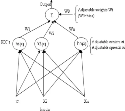
Radial functions are simply a class of functions. In principle, they could be employed in any sort of model (linear or nonlinear) and any sort of network (single-layer or multi-(single-layer). However, since Broomhead and Lowe's seminal paper, radial basis function networks (RBF networks) have traditionally been associated with radial functions in a single-layer network such as shown in Fig. 1.
Radial basis function network (RBFN) can be used successfully to forecast distribution load demands. The RBFN was reported to be more accurate and less time consuming [ISI. As the input variables pass direct to hidden layers without weights, the RBFN models are simpler compared to BP models? The main problem associated with the use of back propagation in forecasting is its slow convergence, difficulty in generalization and arbitrariness in network design. The RBFN was found to overcome these limitations to a certain extent and was shown to give better results. The global modeling and load modeling are done using RBFNs. The RBFN consists of an input layer and hidden layer of high enough dimensions. The output layer supplies the response of the network to the activation patterns applied to the input layer. In the application of RBFN in global modeling, the observations used to train the model of the load values. The training phase constitutes the optimization of a fitting procedure based on the known data points.
The key to a successful implementation of these networks is to find suitable centers for the Gaussian function [10].
Fig. 1Redial Basis Function Network.
2 The steps of long-term load forecasting using neural network
Fig. 2 describes the steps of long-term load forecasting.
For running the RBFNs program, all of the input data (describes in part 3) are used as interiors of RBFNs formula. The program should be designed user friendly for users. After finishing progress, the LSE error should be calculated to recognize that the result is correct or not. If it is not correct, it means that the neural network training shouldn't have done precisely and it should be done again.
3 Selections of proper economy factors
A selection of related parameters as economic factors for long-term load forecasting shows the following factors. These factors were selected very carefully. They
Fig. 2The steps of long-term load forecasting.
have big influence on consumption. All of these factors have their actual data and they are collected from 1989 up to 2007. These factors are later used as inputs to the networks.
3.1 Selected Economy Factors
a) Gross Domestic Product (GDP). GDP shows
the size of economic activity and economic conditions that occur within a country. In view of the increase
b) Population. It is thought that the demand for the
electric power will increase in proportion to the population.
c) Number of households. Households are taken
into account as an important input, because of the existence of many appliances in each household.
d) Hot days. The temperature causes an effect of
electric power demand. In the hot days people usually use cooler, which causes a big share of power consumption. And thus the number of hot days is taken as an input of the Network.
e) Index of Industrial Production (IIP). The entire
industry movement can be achieved by using IIP as input.
f) Electricity price. It is thought that when the
price of electricity is decreases, the amount of useless electric power consumption increases gradually.
g) Maximum Electric Power .The maximum
electric power of the previous year is also used as one of the inputs of the network.
Note: All of the above factors are obtained from some
actual resources such as, TAVANIR Co. and The Library of Central Bank of Islamic Republic Iran.
3.2 Contribution Factor
In this paper, an additional important approach called “Contribution Factor “is presented to determine the level of influences of selected inputs on output. The contribution factor is the sum of the absolute values of the weights leading from the particular variable. Entire data set is checked before training the RBFNs. This function produces a number for each input variable called ”a contribution factor” that is a rough measure of the importance of that variable in predicting the network’s output relative to the other input variables in the same network. The higher the number, the more the variable is contributing to the prediction.
We can use the contribution factor to decide which variable to remove in order to simplify the network and make the training faster. However, we should probably only do this when the number of inputs exceeds 100 for so. It should be noted that the value of a contribution factor should not be considered “gospel” when deciding whether to include a variable in a network. Neural networks are capable of finding patterns among variables
Start
Select Neural Network type
Select Economic Factors
Learning
Saving the Result
Run Forecasting
Run
Output Control
Result
Finish Yes
No
when none of the variables themselves are highly correlated to the outputs. Obviously, if a certain variable is highly correlated with the output, the variable will have a high contribution factor. The number of input variables also affects the contribution factor. For example, if we include more than 60 to 80 input variables, sometimes the contribution factors get very close to each other and we cannot differentiate among the variables.
The contribution factor of remaining inputs is shown in Fig. 3. The Y-axis of this Fig. 3 shows the percentage of the influence of each input on the output.
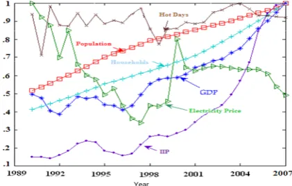
3.3 Normalized Economy Factors
The economy factors which were selected had different scales. For using these economy factors in a same network, we should normalize them between 0.1 and 0.9. Fig. 4 shows the diagram of normalized economy factors. These normalized economy factors have been drown in MATLAB.
4 Design OF Radial Basis Function Networks for Long-Term Load Demand Forecasting
A Radial Basis Function Network (RBFN) in most general terms is any network, which has an internal representation of hidden processing elements (pattern units) which are radically symmetric. For a pattern unit to be radically symmetric, it must have the following three constituents:
• A center, which is a vector in the input space
and which is typically stored in the weight vector from the input layer to the pattern unit.
• A distance measure, to determine how far an
input vector is from the center. Typically, this is the standard Euclidean distance measure.
• A transfer function, which is a function of a
single variable, and which determines the output of the PE (processing elements) by mapping the output of the distance function. A common function is a Gaussian function, which outputs stronger values when the distance is small.
In other words, the output of a pattern unit is a function of only the distance between an input vector and the stored center. The network architecture, characteristics and the learning strategy of RBFNs will be described in the following section.
4.1 Network Architecture of Radial Basis Function Networks
RBFNs consist of three layers; the input layer, hidden layer and output layer. The nodes within each layer are fully connected to the previous layer, as shown in Fig. 5.
In the present work, there is one input layer, one hidden layer and one output layer, as shown in Fig. 5. Six input neurons, six hidden neurons and one output neuron are found to be an adequate combination to give reasonably good training results. The yearly load and economy factors data collected. To start with, the economy factors data for first year form the input set and load data for the first year is taken as the output for training purposes. Similarly the second training data set is obtained from the second year (input) and the load data for the second year (output). The model validation is done by finding the forecast error and the confidence interval for the network forecast and is to be within limits.
The output of the network is given by the following equations.
T
Aw=H y (1)
1 T
w=A H y− (2) where;
1 T 1
A− =(H H)− (3)
y=wH (4)
where, H is a matrix consists of h(x) as Gaussian functions and w is the weight between output & hidden layer.
97.37
25.52
94.24 99.41 94.90
33.59
0 20 40 60 80 100 120
GDP Electricity Price
Population # of Households
IIP Hot Days
[%]
Fig. 3Contribution factor of the selected inputs.
Year
Fig. 4Normalized Economy Factors.
Fig. 5The architecture of RBFNs model.
We can describe H as the following matrix:
(5)
And h(x) is;
(6)
where, r is the variance of Gaussian function.
The input layer consists of n units which represents the elements of the vector x. The links between input and hidden layer contain the elements of the vectors Cj.
The hidden units compute the Euclidean distance between the input pattern and the vector, which is represented by the links leading to this unit. The activation of the hidden units is computed by applying the Euclidean distance to the function h(x).
4.2 Characteristics and Learning Strategy of Radial Basis Function Networks
RBFNs have static Gaussian function as the non-linearity for the hidden layer processing elements. The Gaussian function responds only to a small region of the input space where the Gaussian is centered. The key to a successful implementation of these networks is to find suitable centers for the Gaussian functions. This can be done with supervised learning.
We set suitable centers for the Gaussian functions and after that by using least square error (LSE), we can find the best variance for Gaussian functions.
The centers of Gaussian functions are determined as the mean of each group of economy factors.
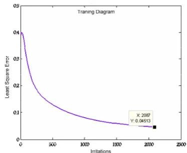
Fig. 6 shows the training diagram of Radial Basis Function network. It is obvious, after 2087 irritations the percentage of least square error decreases fewer than 4.5%.
The advantage of the RBFNs is that it finds the input to output map using local approximations. From the
characteristics of RBFNs, we perceived that it is possible to obtain a better solution for prediction type problem with a large number of inputs. In long-term load forecasting, it is usually used a huge quantity of data which is suitable for RBFNs architecture. Thus, RBFNs is proposed for long-term load forecasting.
5 RBFNS simulations and results
Here the years 2007 to 2011 had been taken as target years to predict the loads. The error calculation of RBFNs is shown in Table 1. The training years are taken years from the year 1989 to 2006. Here shows the training error (LSE) is 4.45%.
The proposed method is examined by using the real data from the year 1989 for forecast the yearly peak load, sine the proposed peak load models is largely dependent on forecast economy factors.
Fig. 7 shows the actual load and estimated load from 1989 to 2006 by RBFNs. All of the data are normalized.
The validation years are selected randomly from 1998 to 2004. Table 2 shows the error of validation years by RBFNs.
After training RBFNs, the neural network is available for forecasting the future years. The years 2007 to 2011 had been taken as target years to predict the loads. Table 3 describes the forecasted load by RBFNs.
Fig. 8 shows the actual load and forecasted load together.
Note: All of the actual loads are obtained from TAVANIR Co.
6 Comparisons Between RBFNs and Multiple Linear Regression (MLR) Forecasting
In this paper, the proposed RBFNs peak load models forecast are compared with the estimation using a linear combination of independent variables. The application of general case of statistical forecasting method involves basic tasks analyze the data series and selection of the forecasting model. A Multiple Linear Regression (MLR) model shown in (7) can be represented as:
Fig. 6 The training diagram.
1 1 m 1
1 n m n
h (x ) h (x )
H
h (x ) h (x )
⎛ ⎞
⎜ ⎟
= ⎜ ⎟
⎜ ⎟
⎝ ⎠
K M O M
L
2 j
(x c )
h(x) exp( )
r − − =
0 0.1 0.2 0.3 0.4 0.5 0.6 0.7 0.8 0.9
1989 1990 1991 1992 1993 1994 1995 1996 1997 1998 1999 2000 2001 2002 2003 2004 2005 2006 Year Normalized Load
Actual Load Estimated Load
Fig. 7 Actual load and estimated load from 1989 to 2006 by
RBFNs.
0 5000 10000 15000 20000 25000 30000 35000 40000 45000 50000
19891990199119921993199419951996199719981999200020012002200320042005200620072008200920102011 Forcasted Load
Actual Load
Fig. 8 Forecasted load from 2007 to 2011 by RBFNs.
Fig. 9 Comparisons between RBFNs and MLR forecasting.
1 0 1 1 2 2 m m
Y =a +a X +a X + +... a X +e
(7)
where Y1 is the forecast variable, X1−Xm are the
explanatory variables, a0−am are the linear regression
coefficients, and the error term. This function can represent the explanatory of the variable as the length of a data set in 18 years from (1989-2006), and Fig. 9 describes the comparisons between RBFNs and MLR forecasting. Table 4 shows the MLR results.
Table 1 RBFNs Error Calculation.
Year Actual
Load*
Estimated
Load* Error %Error
1989 0.20 0.24 0.04 4.39
1990 0.22 0.21 -0.02 -1.89
1991 0.24 0.26 0.01 1.43
1992 0.26 0.31 0.04 4.28
1993 0.29 0.25 -0.04 -3.97
1994 0.31 0.28 -0.04 -3.6
1995 0.33 0.30 -0.03 -3.04
1996 0.35 0.36 0 0.36
1997 0.38 0.40 0.02 2.08
1998 0.41 0.39 -0.02 -1.71
1999 0.43 0.43 0 0.18
2000 0.47 0.48 0.01 1.5
2001 0.50 0.52 0.01 1.32
2002 0.54 0.51 -0.03 -2.63
2003 0.59 0.57 -0.03 -2.72
2004 0.64 0.68 0.04 3.81
2005 0.70 0.75 0.04 4.24
2006 0.75 0.83 0.08 8.04
*Normalized Data
Table 2 Validation of RBFNs.
Year Actual
Load*
Estimated
Load* Error %Error
1998 0.55 0.64 0.08 8.34
2000 0.63 0.64 0.02 1.72
2002 0.73 0.65 -0.08 -7.66
2004 0.86 0.85 -0.01 -0.54
*Normalized Data
Table 3 Forcasted load by RBFNS.
Year Forecasted Load(MW)
2007 38097
2008 43461
2009 46083
2010 47643
2011 48337
Table 4 Forcasted load by MLR.
Year Forecasted Load(MW)
2007 37064
2008 40431
2009 42231
2010 43831
2011 45431
7 Conclusions
Electric power companies expect to have adequate generating and transmission capacity resources for the several years ahead. Generally, the amount adequate generating and transmission capacity resources come from the results of mid and long-term load forecasting. However, mid- and long-term forecasts are not always accurate; therefore the power companies are always worried about this issue. Regarding this issue, we have developed some models for accurate load forecasting of couple of years ahead. It has been demonstrated in this paper that the proposed RBFNs give relatively accurate load forecasts for the actual data. One of the important points for forecasting the long-term load in Iran is to take into account the past and present economic situations and power demand. These points were considered in this study. The proposed RBFNs have also showed that the changes in loads are a reflection of economy.
Based on the results obtained from this study, we determined that the loads are increasing with mean annual incremental rate of about 5.35% up to year 2011. The reason is because very recently there took place a big brake in economy development in Iran. As far as the economy in near future is concerned, return to the former condition will not be simple for Iran.
Here, this study is not intending to go further than this point. What is trying to mention in this paper is that the loads will grow to a certain point for 5 to 10 years ahead. These fluctuations in long-term loads may bring this question that we may not be able to forecast the loads for very long periods. The answer to this question is to provide a sense of security to the power companies, a sensitivity analysis for load deviations and many variables, which may cause these fluctuations. That means, we must not only rely on the forecast of very long period, but also consider that as a reference or rough forecasting and then correct our forecasted curves by new coming information.
References
[1] Al Mamun M. and Negasaka K., “Artificial
neural networks applied to long-term electricity demand forecasting,” Proceedings of the Fourth International Conference on Hybrid Intelligent Systems(HIS'04), pp. 204–209, Dec 2004.
[2] Khoa T. Q., and Oanh P. T. , “Application of
Elman and neural wavelet network to long-term load forecasting,” ISEE journal, track 3, sec. B, No. 20, 2005.
[3] Al-Hamidi H. M. and Soliman S.A.,
“Long-term/mid-term electric load forecasting based on short-term correlation and annual growth”, Electric power system research (Elsevier), Vol. 74, No. 3, pp. 353-361, June 2005.
[4] Negasaka K. and Al Mamun M., “Long-term
peak demand prediction of 9 Japanese power utilities using radial basis function networks,”
IEEE power engineering society general meeting, Vol. 1, pp. 315-322, June 2004.
[5] Engineering and design hydropower proponent,
Load forecasting methods, in EM 110-2-1701, Dec 1985, Appendix B.
[6] Genethliou D. and Feinberg E. A., Load
forecasting, Applied mathematics for restructured electric power system: optimization, control and computational intelligence, (J. H. Chow, F.F. Wu, and J.J. Momoh, eds.), chapter 12, pp. 269-285, 2005.
[7] Fu C. W. and Nguyen T. T., “Models for
long-term energy forecasting”, IEEE power engineering society general meeting, Vol. 1, pp. 235-239, July 2003.
[8] Taradar Heque M. and Kashtiban A.M.,
“Application of neural networks in power systems; A review,” Transaction of engineering, computing and technology, Vol. 6, ISSN 1305-5313, pp. 53-57, June 2005.
[9] Atiya A. F., “Development of an intelligent
long-term electric load forecasting system,” Proceedings of the International Conference, ISAP apos, pp. 288-292, 1996.
[10] Kermanshahi B. S. and Iwamiya H., “Up to year
2020 load forecasting using neural nets”, Electric power system research (Elsevier), Vol. 24, No. 9, pp. 789-797, 2002.
[11] Phimphachanh S., Chamnongthai K., Kumhom P.
and Sangswang A., “Using neural network for long term peak load forecasting in Vientiane
municipality,” IEEE region 10 conference,
TENCON 2004, Vol. 3, pp. 319-322, 2004.
[12] Khoa T. Q. D., Phuong L. M., Inh P. T. T. B.,
Lien N. T. H., “Application of wavelet and neural network to long-term load forecasting,” International conference on power system technology (POWERCON 2004), pp. 840-844 Singapore, 21-24, Nov. 2004.
[13] Khoa T. Q. D., Phuong L. M., INH P.T.T.B, Lien
N. T. H., “Power load forecasting algorithm based on wavelet packet analysis”, International conference on power system technology (POWERCON 2004), pp. 987-990, Singapore, 21-24, Nov. 2004.
[14] EL_Naggar K. M. and AL-Rumaih K. A.,
“Electric load forecasting using genetic based algorithm, optimal filter estimator and least error square technique: Comparative study,” Transaction of engineering, computing and technology, Vol. 6, pp. 138-142, ISSN 1305-5313, June 2005.
[15] Pai P. F. and Hong W. C., “Forecasting regional
electricity load based on recurrent support vector machines with genetic algorithms,” Electric power system research (Elsevier), Vol. 74, pp. 417-425, 2005.
[16] Faraht foreca techniq Interna confer 2004. [17] Kandil E., “Th strateg system (Elsev [18] Carmo Antoni foreca annua society
t M. A., sting and pla que and fuz ational univ rence, UPEC
l M. S., El-D he implement gies using
m: part-II,” El
ier), Vol. 58, ona D., Jaram
io A. J., sting with ne l conference y, Vol. 3, pp. 1
“Long-term anning using zzy interface versities pow 2004, Vol. ebeiky S.M. tation of
long-a knowledg lectric power pp. 19-25, 20 millo M.A., G
“Electric e eural network of the indus 1860-1865, 20
industrial l neural netwo
method,” 3
wer engineer 1, pp. 368-3
and Hasanien -term forecast ge-based exp system resea 01. Gonzalez E. energy dem
ks,” IEEE, 2
strial electron 002. load orks 39th ring 372, n N. ting pert arch and mand 28th nics pow Exc has 100 inc Gen stab wer installation
cellence for Po s around 30 Jo 0 papers at Inte lude wind an nerations, pow bility and optim
Ladan Ghod 1980. She re Azad Univer in power en university o (IUST) in neural netwo the future fa n especially in in
Mohsen Ka Iran. He rec Institute of T in 1991. D Associate Pr Electrical En of Science an also foundi ower System A ournal publicati ernational Conf nd solar pow wer system dy mization.
ds was born in eceived her B. rsity of Tehran. ngineering in M
of science an 2008. She is ork and its abili
ctors. She is als ndustries.
alantar, was bo
ceived his Ph.D Technology, Ne Dr. Kalantar is rofessor in the ngineering at I nd Technology ing member Automation and
ions and has p ferences. His fi wer generation ynamics and c
Tehran, Iran in S degree from . She graduated M.S from Iran nd technology interested in ities to forecast so interested in
orn on 1961 in D. from Indian ew Delhi, India s currently an Department of Iran University y, Tehran. He is of Center of Operation. He presented about elds of interest ns, Distributed ontrol, system n m d n y n t n n n a n f y s f e t t d m