A MODEL FOR MIXED CONTINUOUS AND DISCRETE RESPONSES WITH POSSIBILITY OF MISSING RESPONSES

A MODEL FOR MIXED CONTINUOUS AND

DISCRETE RESPONSES WITH POSSIBILITY OF

MISSING RESPONSES

M. Ganjali

Department of Statistics, Faculty of Mathematical Sciences, Shahid Beheshti University, Evin, Tehran 19838, Islamic Republic of Iran

Abstract

A model for missing data in mixed binary and continuous responses, which can

be used on cross-sectional data, is presented. In this model response indicator for

the binary response can be dependent on the continuous response. A closed form

for the likelihood is found. For data with a complicated pattern of missing

responses some new residuals are also proposed. The model of multiplicative

heteroscedasticity is used to consider the problem of heteroscedasticity of the

continuous response. The model is illustrated on the data of an observational study

where the effect of psychological disorder of parents on both the verbal

comprehension score and the presence of adverse symptoms in their children are

modeled in the presence of missing responses.

Keywords: Mixed data; Missing responses; Multiplicative heteroscedasticity; Pearson residuals; Psychological disorder

* _{E-mail: [email protected]} 1. Introduction

Some biomedical, psychological and health sciences data include both discrete and continuous outcomes. One example is the analysis of development toxicity endpoints when the relationship between fetal weight and malformation in live fetus is an important statistical issue [1]. Another example is, in the study of the maternal smoking effect on respiratory illness in children where we have a continuous measure of pulmonary function and a binary measure of chronic symptoms in children.

For the first example, separate analyses of the categorical or the continuous responses cannot properly

assess the effect of dose on fetal weight and malformations simultaneously. For the second example, separate analyses cannot assess the effect of maternal smoking on all the responses simultaneously. Furthermore, separate analyses give biased estimates for the parameters and misleading inference [9]. Consequently, we need to consider a method in which these variables can be modeled jointly.

continuous variables, given the categorical variables. Another method is to consider the conditional distribution of discrete variables, given the continuous variables and a marginal distribution for continuous variables. Cox and Wermuth [2] empirically examined the choice between these two methods. The third method which is developed here is to use simultaneous modeling of categorical and continuous variables to take into account the association and dependence between the responses by the correlation between the errors in the models for responses. For more details of this approach see, for example, Heckman [6] in which a general model for simultaneously analyzing two mixed correlated responses is introduced and Catalano and Ryan [1] who extend and used the model for a cluster of discrete and continuous outcomes.

Little and Rubin [10] made an important distinction between the various types of missing mechanism. They defined the missing mechanism as missing completely at random (MCAR) if missingness is dependent neither on the observed responses nor on the missing responses, and as random (MAR) if it is dependent on the observed responses, but not on the missing responses. Missingness is defined as non-random if it depends on the unobserved responses. From a likelihood point of view MCAR and MAR are ignorable but missing not at random (MNAR) is non-ignorable.

For mixed data with missing outcomes, Little and Schluchter [11] and Fitzmaurice and Laird [3] used the general location model of Olkin and Tate [14] with the assumption of missingness at random (MAR) to justify ignoring the missing data mechanism [10]. This means that they used all available responses, without a model for missing mechanism, to obtain parameter estimates using the EM (Expectation Maximization) algorithm. For a good discussion of mixed normal and non-normal data with missing responses under the assumption of MAR, see [10] and [16].

In this paper a general latent variable model for simultaneously handling response and non-response in mixed discrete and continuous data with potentially nonrandom missing values in both types of responses is presented. With this model, the dependence between responses can be taken into account by the correlation between errors of the response models. The aim is to use the general model of Heckman [6] for the joint modeling of the discrete and continuous responses. It is shown how we can incorporate a model for a complicated pattern of missing responses.

In Section 2, the model is described and some new residuals are introduced. In Section 3, this model is used on a subset of data available in Little and Schluchter [11] about the effects of parental psychological

disorders on various aspects of the development of their children. The results of fitting this model are also presented. In Section 4, the paper concludes with some remarks.

2. Model and Residuals for Mixed Data with Missing Responses

2.1. The Model

Suppose y is a binary discrete variable and z is a continuous variable. Variables y and z are correlated and must be modeled simultaneously. Let y*_{, R}*

y and R*

z denote the underlying latent variables of the binary response, the non-response mechanism for the binary variable and the non-response for the continuous variable, respectively, and define

Ry = ⎩ ⎨

⎧ 〉

, 0

0 1 *

Otherwise R

if _y

as the response indicator for y,

Rz = ⎩ ⎨

⎧ 〉

, 0

0 1 *

Otherwise R

if _z

as the response indicator for z and

y = ⎩ ⎨

⎧ 〉

, 0

0 1 *

Otherwise y if

as the binary response. The model takes the form: ,

1 1 1 * _{=β′X +ε}

y (1a)

,

2 2

2 σε

β′ +

= X

z (1b)

,

3 3 1 * _{=α′X +ε}

R_y (1c)

4 4 2 *_{=α′X +ε}

R_z , (1d)

where Xj for j=1,2,3,4 are vectors of explanatory variables. It is assumed that E(εj)=0 for j=1,...,4. The unstructured (us) variance covariance matrix of the vector of errors

(

)

∑

⎟⎟ ⎟ ⎟ ⎟

⎠ ⎞

⎜⎜ ⎜ ⎜ ⎜

⎝ ⎛

=

us

1 1 1 1

34 24 14

34 23 13

24 23 12

14 13 12

ρ ρ ρ

ρ ρ ρ

ρ ρ ρ

ρ ρ ρ

4 ,..., 2

= ′

j should be estimated. In this model any multivariate distribution can be assumed for the errors in the model. Here a multivariate normal distribution is assumed.

To consider the problem of heteroscedasticity of the continuous response we can use multiplicative model of heteroscedasticity [5] for σ which is

(

exp γ0 γ

)

σ = + ′ (1e)

where γ0 and the vector of parameter γ should be estimated and X is the vector of explanatory variables.

The non-response of y (Ry) in this model depends on both responses, the non-response for z (Rz) also depends on both responses and z depends on y. If, one of the correlation parameters ρjj′ for j=1,2 and j′=3,4 is found

to be significant, then we have a nonrandom missing process. Parameter ρ₁₄ (ρ₂₃) can tell us whether or not non-response in the continuous variable (binary variable) is dependent on response in the discrete variable (continuous variable). Parameter ρ34 can tell

us whether or not non-response in the continuous variable is dependent on the non-response in the discrete variable.

The likelihood for this model, which has been given in appendix, shows the simplification obtained by using the assumption of normality in the models for non-response. The simplification arises from the fact that, instead of resorting to a numerical approximation of the integral needed to integrate out the missing values of the continuous response, we just need to invoke a point on the cumulative three-variate normal distribution, which although approximate, can be computed in many standard statistical packages with sufficiently high precision.

The NAG [13] routine EO4UCF is used in this paper to minimize the mines logarithm of the likelihood given in the appendix. EO4UCF is a Fortran routine to minimize a smooth function subject to constraints (for example simple bounds on the variables) using a sequential quadratic programming (SQP, [4]) method. In this routine all unspecified derivatives are approximated by finite differences.

2.2. Residuals

The missing values of responses create problems for the usual residual diagnostics, see e.g. Hirano et al. [8]. For example usual Pearson residuals of the z variable are of the form

) var(

) (

Z z E z

r_z = −

i.e. they assume MCAR. These unconditional residuals will be misleading if missingness is MAR or MNAR as in these cases the z's are from a conditional or truncated conditional distribution. We can examine the residuals of the responses conditional on being observed. Let start with using theoretical form, involving E(ZR_z =1),

) 1 (Y Ry=

E and var(ZR_z =1) rather than their predicted values. The Pearson residuals for continuous response can take the form

) 1 var(

) 1 (

= = −

=

z z z

R Z

R Z E z

r (2a)

and for the discrete response can take the form

(

)

(

)

(

(

)

)

1

= −

× =

= −

=

y y

y z

R Y E R

Y E

R Y E y

r (2b)

where

M, σρ X β ) R

E(Z Z=1 = 2′ 2+ 24

(

)

(

)

[

]

4 2 2 24 2 24

2 _{1 1}

1

var(ZR_Z = )=σ −ρ +ρ −Mα′X −M

(3)

where

(

)

(

)

α α

′ Φ

′ − Φ

= is the Mill's ratio [7,12] and

(

)

(

)

E

(

)

(

)

(

(

)

)

3 3 1

1

1

; , , 1

X

X X X

X

α

ρ α β α

β

′ − Φ −

′ − ′ − Φ + ′ − Φ − ′ − Φ − =

(4) where Φ and Φ12 are respectively the cumulative

univariate and bivariate normal distributions.

The estimated Pearson residuals can be found by using the maximum likelihood estimates of the parameters in System (1). As residuals in (2a) and (2b) are defined by conditioning on observing the responses, they differ from those of Ten Have et al. [15]. Ten Have et al. [15] found the expectation and variances of responses, and consequently the residuals, unconditional on the fact that responses should be observed. Then, to calculate the residuals they assumed no link between

response and nonresponse. This gives biased estimates of the means and variances of responses if missingness is not at random [10].

3. Application: The Effect of Psychological Disorders on the Verbal Comprehension Score

3.1. Psychological Disorders Data

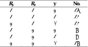
The data set extracted from Little and Schluchter [11] has been used also by Fitzmaurice and Laird [3]. These authors assumed a mechanism by which observations were MAR and then used the general model of Olkin and Tate [14] to decompose the joint distribution of the continuous and discrete variables. In these data, school-age children are classified according to the risk of their parents to psychological disorders (normal, moderate risk and high risk). Little and Schluchter [11] and Fitzmaurice and Laird [3] used two continuous responses, a standardized reading score and a standardized verbal comprehension score, and a single binary response, indicating the presence of adverse symptoms, which was obtained for each child. Here, only the standardized verbal comprehension score and the binary response for the first child in family are used. The data include 69 families with a general pattern of missing responses. Table 1 gives the different patterns of missing response for each child.

For example, 15 first-born children responded for both variables and the observed value of their binary response is 0.

Since a preliminary analysis indicated that there was no significant difference between moderate and high risk groups of psychological disorders [3], in this paper, the moderate and high risk groups are combined into a single group.

Table 1. Different patterns of missing responses for psychological disorders data

Ry Rz y No.

1 1 0 15 1 1 1 12 0 1 - 12 1 0 0 6 1 0 1 8 0 0 - 16

Table 2. Descriptive statistics for psychological disorders observed data

Score Ad. Sym

Low

Risk No mean S.D. 0 1 Total

0 22 105.455 30.764 10** _{(24.4) 11(26.8) 21(51.2)}

1 17 146.118 19.647 16(39) 4(9.8) 20(48.8) Total 39 123.176* _33.210* _{26(63.4) 15(36.6) 41} * _{Calculated ignoring low risk,} ** _Count(%)

Table 2 presents summary statistics for presence of the adverse symptoms (Ad. Sym. in Table 2) and the standardized verbal comprehension score using only observed data. In this table the value of 0 for ‘Low Risk’ means that we have an individual from moderate or high risk group and the value of 1 means that individual is from low risk group.

Table 2 shows that the mean (standard deviation) score of children from a family with a low risk of psychological disorders (Low Risk=1 in Table 2) is more (lower) than families with moderate or high risk of psychological disorders. It also shows that the occurrence of adverse symptoms is less in family with a low risk of psychological disorders.

As the variance of scores is less for a family with a low risk of psychological disorders, the problem of heteroscedasticity should be taken into account.

A Kolmogorov Smirnov test of the assumption of normality for scores of the children of a low family of psychological disorders is not rejected (p-value=0.200). The same test does not reject the assumption of the normality for scores of the children from a moderate or high risk of psychological disorders (p-value=0.200). The Pearson correlation between two responses is r=−0.449. This emphasizes that two responses should be modeled simultaneously.

3.2. Models for Psychological Disorders Data

For comparative purposes, three models are considered. The first model (model I) uses only complete cases and does not consider the correlation between two responses. This model is

,

1 11 01

*_{=β +β L+ε}

y (5a)

,

2 12

02 β σε

β + +

= L

z (5b)

(

)

expγ γ

σ = + (5c)

where there is no correlation between ε₁ and ε₂. The second model (model II) uses model I and takes into account the correlation between two responses. The third model (model III) considers the full model, model with missing mechanism, with the following form

,

1 11 01

*_{=β +β L+ε}

y (6a)

,

2 12

02 β σε

β + +

= L

,

3 21 11 01

* _{=α +α L+α M+ε}

R y (6c)

,

4 22 12 02

*_{=α +α L+α M +ε}

Rz (6d)

(

expγ γ

)

σ = + . (6e)

In these models

⎩ ⎨ ⎧ =

Otherwise 0

group risk low a from is child if 1 L

and

⎩ ⎨ ⎧ =

Otherwise 0

group risk Moderate a

from is child if 1 M

In model (III) non-response models (R*

y and R*z) let

have one more explanatory variable [6].

3.3. Results for Psychological Disorders Data

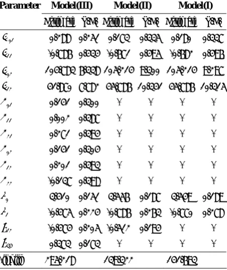
For the standardized verbal comprehension score and the binary response for the first born child in family, model (III) finds no connection between missing mechanism and responses with a change of deviance of 2.4116 on 4 d.f. (p-value=0.661). Consequently, using only the complete data, without considering the missing mechanism, can give unbiased estimates of the parameters. Results of using three models are given in table 3. For model (III) as the correlation parameters

j j′

ρ for j=1,2 and j′=3,4 are not significant (as mentioned above) results with removing these parameters are given.

These results show that there is a negative correlation (a change in deviance of 4.742 with 1 df) between two responses (the more the score the less likely the presence of adverse symptoms) and separate analysis of the responses gives biased estimates of the standard errors of the parameters. For example, under model (I), the standard errors of the estimates of β02 and β12, in comparison with the results of the model (II), are overestimated and the standard errors of the estimates of β01 and β11 are underestimated. Results also show that children from a low risk family can obtain a better standardized verbal comprehension score and the variance of their scores is less than that of the family with a high or moderate risk (γ1=−0.786 for model II).

The estimate of the parameter by model (III) shows a positive correlation between two underling variables for missing mechanisms. This means that children who do not respond their score are more likely to not to respond their discrete response.

Table 4 shows values of residuals calculated using

(2b) and model (II) for the discrete response.

Residuals for continuous response calculated using (2a) do not include any value larger than 3 (in absolute value) and with the residual values in Table 4, model (II) can be considered as a good fit for the psychological disorders data.

Table 3. Results using three models for the psychological disorders data

Parameter Model(III) Model(II) Model(I)

Estimate S.E. Estimate S.E. Estimate S.E.

01

β 0.288 0.251 0.173 0.335 0.180 0.337

11

β -0.786 0.434 -0.671 0.495 -0.682 0.496

02

β 104.783 6.338 105.214 9.300 105.214 9.297

12

β 41.870 7.782 45.786 10.341 45.786 10.315

01

α 0.141 0.300 - - - -

11

α 0.002 0.387 - - - -

21

α 0.271 0.394 - - - -

02

α 0.141 0.304 - - - -

12

α 0.201 0.393 - - - -

22

α -0.137 0.398 - - - -

0

γ 3.410 0.151 3.556 0.187 3.549 0.189

1

γ -0.475 0.224 -0.786 0.263 -0.770 0.278

12

ρ -0.474 0.205 -0.512 0.194 - -

34

ρ _{0.373 0.173 - - - -}

-loglik 295.218 139.322 141.693

Table 4. Residuals for discrete response using model (II) for psychological disorders data

Y=0 Y=1 L=0 -0.871 1.149 L=1 -1.494 0.670

4. Discussion

response indicators should be defined and the more parameters coming to the estimation procedure.

The selection models in systems (1) can be sensitive to the assumption of normality for error distributions [10]. However, the residuals introduced in this paper can be used to practically examine this assumption.

Acknowledgments

The author is grateful to Shahid Beheshti University for the awarded research grant.

References

1. Catalano P. and Ryan L.M. Bivariate latent variable models for clustered discrete and continuous outcomes.

Journal of the American Statistical Association, 87(419): 651-658 (1992).

2. Cox D.R. and Wermuth N. Response models for mixed binary and quantitative variables. Biometrika, 79(3): 441-461 (1992).

3. Fitzmaurice G.M. and Laird N.M. Regression models for mixed discrete and continuous responses with potentially missing values. Biometrics, 53: 110-122 (1997).

4. Fletcher R. Practical Methods of Optimization. John Wiley (2000).

5. Harvey A. Estimating regression models with multiplicative heteroscedasticity. Econometrica, 44: 461-465 (1976).

6. Heckman J.J. Dummy endogenous variables in a simultaneous equation system. Econometrica, 46(6): 931-959 (1978).

7. Heckman J.J. Sample selection bias as a specification error. Ibid., 47: 153-161 (1979).

8. Hirano K. Imbens, G. Ridder, G. and Rubin, D. Combining panel data sets with attrition and refreshment samples. Technical working paper, National Bureau of Economic Research. Cambridge, Massachusetts (1998). 9. Leon A.R. and Carriere K.C. On the one sample location

hypothesis for mixed bivariate data. Commun. statist. Theory and Meth., 29(11): 2573-2581 (2000).

10. Little R.J and Rubin D. Statistical Analysis with Missing Data. New York; Wiley (1987).

11. Little R.J. and Schluchter M. Maximum likelihood estimation for mixed continuous and categorical data with missing values. Biometrika,72(3): 497-512 (1985). 12. Maddala G.S. Limited dependent and qualitative

variables in econometrics. Cambridge, (1983).

13. NAG. Numerical Algorithms Group Manual. Mark 16. Oxford, U.K. (1996).

14. Olkin I. and Tate R.F. Multivariate correlation models with mixed discrete and continuous variables. Annals of Mathematical Statistics, 32: 448-465 (1997).

15. Ten Have T.R.T., Kunselman A.R., Pulkstenis E.P., and Landis J.R. Mixed effects logistic regression models for longitudinal binary response data with informative drop-out. Biometrics, 54: 367-383 (1998).

16. Schafer J.L. Analysis of Incomplete Multivariate Data, Chapman & Hall (1997).

Appendix: Likelihood for Mixed Data with Missing Mechanism

For individuals who observe neither y nor z the likelihood is

(

)

Pr = =

= R_y R_z

L

(

)

12 −α′X ,−α′X ;ρ

Φ

= , (7)

where Φ₁₂ is the cumulative bivariate normal distribution.

For individuals who observe only y and the value of y is 0 the likelihood is

(

)

Pr = = =

= y Ry Rz

L

=Pr

(

)

(

)

=Φ₁₂

(

)

−Φ₁₂₃

(

)

where

⎥ ⎥ ⎥

⎦ ⎤

⎢ ⎢ ⎢

⎣ ⎡ = ∑

1 1 1

34 14

34 13

14 13

134

ρ ρ

ρ ρ

ρ ρ

and Φ₁₂₃ is cumulative three-variate normal distribution.

For individuals who observe only y and the value of y is 1 the likelihood is

) 0 , 1 , 1

Pr( = = =

= y R_y R_z

L

=Pr(R_z =0)−Pr(y=0,R_z =0)

−Pr(R_y=0,R_z =0)

+Pr(y=0,R_y=0,R_z =0)

=Φ(−α₂′X₄)−Φ₁₂(−β₁′X₁,−α₂′X₄;ρ₁₄)

−Φ₁₂(−α₁′X₃,−α₂′X₄;ρ₃₄)+

Φ₁₂₃(−β₁′X₁,−α₁′X₃,−α₂′X₄;Σ₁₃₄). (9)

For individuals who observe only z the likelihood is

) 1 , 0 Pr( )

(z R R z

f

L= _y = _z =

− − ′ − − ′ − Φ = ) 1 ) ( ( )[ ( 23 2 2 2 23 3 1 ρ β σ ρ

α X z X

z f , )] 1 1 ; 1 ) ( , 1 ) ( ( 24 2 23 2 23 24 34 24 2 2 2 24 4 2 23 2 2 2 23 3 1 ρ ρ ρ ρ ρ ρ β σ ρ α ρ β σ ρ α − − − − ′ − − ′ − − ′ − − ′ − Φ X z X X z X (10) For individuals with both z and y observed and the

value of y equal to 0 the likelihood is ) 1 , 1 , 0 Pr( )

(z Y R R z

f

L= = _y = _z =

= f(z)[Pr(y=0z)−Pr(Y=0,R_y =0z)

−Pr(Y =0,Rz =0z)

+Pr(Y =0,Ry =0,Rz =0z)]

12 2 2 2 12 1 1 12 12 2 2 2 12 1 1 1 ) ( ( ) 1 ) ( ( )[ ( ρ β σ ρ β ρ β σ ρ β − ′ − − ′ − Φ − − ′ − − ′ − Φ = X z X X z X z f , − − − − − ′ − − ′ − ) 1 1 ; 1 ) ( 23 2 12 2 23 12 13 23 2 2 2 23 3 1 ρ ρ ρ ρ ρ ρ β σ ρ

α X z X

+ − − − − ′ − − ′ − − ′ − − ′ − Φ ) 1 1 ; 1 ) ( , 1 ) ( ( 24 2 12 2 24 12 14 24 2 2 2 24 4 2 12 2 2 2 12 1 1 12 ρ ρ ρ ρ ρ ρ β σ ρ α ρ β σ ρ β X z X X z X , 1 ) ( , 1 ) ( ( 23 2 2 2 23 3 1 12 2 2 2 12 1 1 123 ρ β σ ρ α ρ β σ ρ β − ′ − − ′ − − ′ − − ′ − Φ X z X X z X

(

)

2 2 24 4 2 ∑ − ′ − − ′ − ρ β σ ρ

α X z X

, (11) where ⎥ ⎥ ⎥ ⎥ ⎥ ⎥ ⎥ ⎦ ⎤ ⎢ ⎢ ⎢ ⎢ ⎢ ⎢ ⎢ ⎣ ⎡ − − − − − − − − − − − − − − − − − − = ∑ 1 23 2 1 24 2 1 23 24 34 24 2 1 12 2 1 24 12 14 23 2 1 24 2 1 23 24 34 1 23 2 1 12 2 1 23 12 13 12 2 1 12 2 1 24 12 14 23 2 1 12 2 1 23 12 13 1 2 | 134 ρ ρ ρ ρ ρ ρ ρ ρ ρ ρ ρ ρ ρ ρ ρ ρ ρ ρ ρ ρ ρ ρ ρ ρ ρ ρ ρ ρ ρ ρ

For individuals with both z and y observed and the value of y equal to 1 the likelihood is

) 1 , 1 , 1 Pr( )

(z Y R R z

f

L= = _y = _z =

= f(z)[1−Pr(Y =0z)−Pr(R_y =0z)−

Pr(R_z =0z)+Pr(Y =0,R_y=0z)+

Pr(Y=0,R_z =0z)+Pr(R_y=0,R_z =0z)−

Pr(Y=0,R_y=0,R_z =0z)]

− − ′ − − ′ − Φ − = ) 1 ) ( ( 1 )[ ( 12 2 2 2 12 1 1 ρ β σ ρ

β X z X

z f − − ′ − − ′ − Φ ) 1 ) ( ( 23 2 2 2 23 3 1 ρ β σ ρ

α X z X

+ − ′ − − ′ − Φ ) 1 ) ( ( 24 2 2 2 24 4 2 ρ β σ ρ

α X z X

), 1 ) ( ( 12 2 2 2 12 1 1 12 ρ β σ ρ β − ′ − − ′ −

Φ X z X

; 1 ) ( 23 2 2 2 23 3 1 ρ β σ ρ α − ′ − − ′

+ −

− −

) 1 1 212 223

23 12 13

ρ ρ

ρ ρ ρ

,

1

) (

(

23 2

2 2 23 3 1 12

ρ β σ ρ α

−

′ − −

′ −

Φ X z X

24

2

2 2 24 4 2

1

) (

ρ β σ ρ α

−

′ − −

′

− X z X

;

+

− −

−

) 1

1 224 223 23 24 34

ρ ρ

ρ ρ ρ

12 2

2 2 12 1 1 12

1

) (

(

ρ β σ ρ β

−

′ − −

′ −

Φ X z X ,

24

2

2 2 24 4 2

1

) (

ρ β σ ρ α

−

′ − −

′

− X z X

;

− −

− −

) 1

1 212 224 24 12 14

ρ ρ

ρ ρ ρ

,

1

) (

(

12 2

2 2 12 1 1 123

ρ β σ ρ β

−

′ − −

′ −

Φ X z X

23 2

2 2 23 3 1

1

) (

ρ β σ ρ α

−

′ − −

′

− X z X

,

; )]

1

) (

2 | 134 2

2 2 24 4 2

24

∑ −

′ − −

′ −

ρ β σ ρ

α X z X