Advances in morphometry of soil macroporosity through simple techniques of mathematics

(1)

A b s t r a c t. Soil structure exerts important influences on the soil conditions and this is often expressed as the morphometric measure of its porosity. The measurement systems used until now to evaluate the size, shape, quantity and continuity of the soil pores in two dimensional images at the field scale seem a little outdated. However, the use of image analysis for the purpose has been controversial and it is necessary to improve and standardise some important details of image analysis procedures. Aiming for the separation between round, elongated and irregular pores, it was necessary to create a system of evaluations that would complement the habitually used ‘shape factor’. It was also necessary to include the measurement of other variables, like the diameter, length and width of the complex and irregular cracks that in most cases are impossible to evaluate only with the variables obtained directly from the image analyzers. So, it was necessary to develop and test algebraic equations that would lead to those evaluations. This paper presents a morphometric system that leads to a model of typological classification of soil macroporosity at a field scale. So, this paper contributes toward the normalization of the image analysis techniques, which allows studies to be more rigorous, accurate and quicker, with an acceptable ratio of errors.

K e y w o r d s: image-analysis, macroporosity, soil, field-scale, morphometric evaluation

INTRODUCTION

In many and diversified areas of knowledge it is often necessary to refer to the shape, dimension, identification and classification of several elements. Automated image analy-sis first appeared in the nineteen seventies, through software and hardware integrated in microcomputers (Nawrath and Serra, 1979 a,b; Serra, 1982). In the meantime, throughout

the seventies and eighties, some generic algorithms for image measurement and processing became popular, along with increase in the performance of the personal computer microprocessors. As a consequence of this evolution, the prices of image analysis software are, nowadays, low enough for many scientists to feel attracted to this type of technolo-gy, namely to its application in many aspects of soil science such as the study, in two dimensions, of soil structure inclu-ding porosity. Bullock and Thomasson (1979) and Conway (1980) are examples of users of this type of technology which allows to obtain quantitative data of characteristics that are usually estimated visually (Murphyet al., 1977a,b) or indirec-tly measured, resulting in more rigorous soil descriptions.

The porous space assumes a growing importance in the characterization of soil structure because of the shape, size, quantity and continuity of the pores that affect most of the processes in the soil (Lawrence, 1977) through the influence that they exercise on the dynamics of the structure. That is so important because porosity of a three dimensional (3D) soil block can be adequately predicted using two dimensional (2D) images (Moreauet al., 1999).

In fact, since 1992 until nowadays, a lot of research has been conducted in this direction, including such approaches as fractal analysis (Anderson et al., 2000; Bacchi et al., 1996; Birdet al., 2000; Caniegoet al., 2003) or gas diffusion coefficients (Cousin et al., 1999; Moldrup et al., 2000), among others. However, some important details were for-gotten, and specifically a system of measuring several dimensions to be evaluated in each poroid belonging to the

Advances in morphometry of soil macroporosity through simple techniques

of mathematics

E.P. Sampaio

1,2,3

* and J.M. Sampaio

4

1_{Geosciences Department, University of Évora, Luís António Verney College, Rua Romão Ramalho-5, 7000 Évora, Portugal} 2_{ICAAM, Institute of Mediterranean Agrarian and Environmental Sciences, University of Évora, Núcleo da Mitra, Apt. 94,}

7002-774 Évora, Portugal

3_{CREMINER, Centre for Mineral Resources, Mineralogy and Crystalography, University of Lisbon, Lisbon, Portugal} 4_{CIDEHEHUS, Évora’s University Interdisciplinary Center of History Cultures and Societies, University of Évora,}

Palácio do Vimioso, 7002-554 Évora, Portugal

Received September 25, 2009; accepted January 3, 2010

A

Agggrrroooppphhyhyysssiiicccsss

(2)

soil porous space, including the length and width of highly complex branched pores with irregular thickness and shape. Also, when you want to give specific answers to users, the answers have to be quantitative and rapid. Such responses are only possible if a model based on simple techniques of mathematics is constructed.

Besides, in works on the field scale, it is from sequences of two-dimensional images that one can reconstruct the in-formation onto three dimensions, while other trusted sy-stems in this evaluation type, like computer axial tomo-graphy (TAC) and others, only work on samples of reduced dimensions that are not very representative of the dynamics of reality.

In accordance with several works devoted to the subject shape classification, the poroid shape is usually defined by a circularity index that differs among the authors but which is often estimated by the ratio of the poroid area to its peri-meter (Boumaet al., 1977; Lamandéet al., 2003; Pagliaiet al., 2004), or its shape factor according to Holden (1993). Other authors use two indexes (irregularity and elongation indexes) to describe the morphology of macropores (Ring-rose-Voase and Bullock, 1984; Zida, 1998). However, the approaches developed and selected till now not always really correspond to the reality, which has led to continuing controversy concerning the typological classifications.

According to Skeivalaset al. (2006), the quality of the results of any automatic system of measurement depends on the accuracy and calibration obtained which is considered to be acceptable when the ratio of the measurement error to the calibration is three. So, only based on reliable measurement of the shapes, dimensions and quantities it is possible to ar-rive at conclusions concerning the identity and functionality of elements of this type, like in the case of cracks with com-plex shapes and irregular thickness.

In this work, some improvements were applied at the same kind of indexes (elongation, regularity) to better discriminate the parameterization of each poroid typology. In this way, some of the suggestions by Thompsonet al. (1992), as well as Michell (2005) and Steele and Douglas (2006), were done.

It is intended with this work to contribute some solid pro-posals which will allow to optimize and normalize procedu-res and simple techniques with tools of advanced mathema-tics, for studies that employ two-dimensional images of hori-zontal cross-sections of soil at the field scale. This type of normalization constitutes an effective contribution aimed at elimination of the existing discrepancies between the results and conclusions of different studies on the same subject.

MATERIAL AND METHODS

A poroid data set was derived from horizontal sections of real soil, each of an area of 0.25 m2, impregnated with calcium sulphate and stained blue. Another set of standard forms was used to help with checking some indexes.

According to Hubertet al. (2007), when soil pores are analyzed in vertical sections, typical poroids can be selected and separated into 5 classes as follows:

– tubular poroids (T): near-circular in shape,

– planar poroids (p): elongated in shape, without connection with other poroids,

– discrete packing poroids (Pd): complex in shape, without connection with other poroids in 2D,

– planar packing poroids (Pp): association of variously-shaped poroids with planar connections,

– continuous packing poroids (Pc): complex association of variously-shaped poroids through discrete packing poroids.

Though most of the soil pores can be found to be inter-connected in various ways, when analyzed in two dimen-sional and horizontal images planes they generally appear as discrete objects (Ringroase-Voase and Bullock, 1984), which in turn makes their analysis and quantification easier.

The shape of a poroid can be characterised by some size-independent or dimensionless indexes, as defined by Coster and Chermant (1989). In a two-dimensional macroporosity analysis of soil horizontal planes, three types of pores are regularly identified: circular, elongated and irregular. In this context, the term ‘irregular’ means any shape but circular or elongated (Hubertet al., 2007). Other authors use two inde-xes (irregularity and elongation indeinde-xes) to describe the morphology of macropores (Ringrose-Voase and Bullock, 1984; Zida, 1998). These are often characterised in vertical planes and small samples or thin sections, which is a diffe-rent approach than that employed in this work. Furthermore, this work is concerned with soils that tend to create cracks so large that they need to be studied on a field scale.

The circular pores, often referred to as biopores, are for-med mainly by the soil fauna and/or roots. They consist of cylindrical channels, reaching different depths, and have a particular importance in the water movement and as paths for root development. Many pores of this kind are too wide to promote any soil water retention, but many others play an important role in that respect.

The elongated pores, commonly called cracks, have their origin, in most cases, in natural swelling and shrinkage processes of the mineral clay particles of soil. Cracks may be more or less continuous with depth, depending on the soil degree of contraction. They are dynamically related to the soil moisture content, presenting a tendency to close when the soil wets and to reopen as it dries. Often they are too wide to retain any water but they play an important role in water movement in soil at the beginning of the wetting season.

(3)

increase of the soil water content. Due to their instability, and to the fact that generally they are destroyed as the soil water content rises, and that there is no certainty of their continuity, they are not recognized as having any particular importance in terms of water movement in soil, nor in terms of root penetration, but they may have some importance as far as soil water retention is concerned, depending on their dimensions.

In two-dimensional images, each one of these pore ty-pes shows various sizes. Associated to the size of each one of them, there are many characteristics that can be measured through image analysis, namely area, diameter, length, and width, among others.

In order to perform automatic recognition of the soil pores types by their size and shape using two-dimensional images from horizontal cross-sections, it is necessary to use a specific technology. According to Duff (1977), the statisti-cal recognition technique should be used when the need to recognise the objects is based on certain characteristics that are continuous variables resulting from the measurements taken by the analyzer. Further, according to Coomans and Massart (1981), the statistical classification procedure requi-res the use of a set of n-known objects that are previously classified as standard, in order to have a comparison refe-rence for the objects to be classified. The classification of soil pores takes then the description of each one through a series of variables that represent their characteristics, and subsequen-tly a comparison with the standard objects is performed.

The software used was Sigma Scan Pro, version 4.01 (1996), a ‘Jandel Scientific’ release (now SPSS). This soft-ware allows the realization of studies that require such fun-ctions as morphometric measurements, intensity measure-ments, image processing, data worksheet, graphic results and other features, including:

•morphometric measurements: – distance (strait line and curvilinear), – X, Y co-ordinates,

– area and perimeter, – major and minor axis, – pixel counts,

– shape factor, – Feret diameter; •intensity measurements:

– displaying a histogram of pixel intensities, – pixel intensity measurement,

– measurement of average intensity over an area; •image processing:

– contrast enhancements,

– lookup table and pseudocolour grey and colour trans-formations,

– true and pseudo Clearfield background equalizations; •data worksheet:

– import and export of ASCII files, – output data to a printer,

– store the results of mathematical transformations, – store calibration and lookup table values; •graphing results:

– apply and plot basic statistical functions, – plot X, Y graphs with linear regression; •other features:

– it is noteworthy that this software allows automatic classi-fication of soil pores and cracks, without manual interfe-rence. In order to do that it constructs a table through small built-in programs in its own calculation sheet.

The Sigma Scan Pro software can do various measure-ments of individualised objects including, among others, area, perimeter, Feret’s diameter, and the major and minor axes. Some of these variables, however, should not be measu-red independently from the shape evaluation, because their dimensions depend on it. For example, it does not make sen-se to measure the length or width of a circular shape, nor the diameter of a very elongated one. Thus, the shape recogni-tion is, compulsorily, the first evaluarecogni-tion to be done.

There are various methods for the classification of two-dimensional objects according to their shape. However, most methods comprise a comparison phase between va-riables measured in various shapes and the same vava-riables measured for circular shapes ie they evaluate the proximity to circularity.

According to Holden (1993), the so called shape factor (R) to be used in two-dimensional studies should be the one sup-plied by the ‘Cox’s R-Statistic’ (Cox, 1927). In this,Ris de-fined as:

R= 4p A/P2, (1)

where:Ris the circularity measure,Ais the area, andPthe perimeter of whatever shape.

This formula expresses the existing relationship bet-ween the area of any shape and the area of a circle with the same perimeter. According to Eq. (1)R= 1 for a circle and R= 0 for a line.

Aiming for the separation of round from elongated and from irregular pores, it is necessary, first of all, to define the limits of theRfactor (R= 0 for the circular andR= 1 for the very elongated) which are the values that should work as boundaries to differentiate the three types of pores mentio-ned above. In order to do that, Pettijohn’s Standard Shape Chart (Pettijohn, 1957) was used, taking into account only the circularity component and some well known geometric shapes, as well as their respectiveRfactor values (Fig. 1).

(4)

In order to complete this phase of the study, some samples of soil surfaces, with the pores visible, were photographed and digitalized. Next, some shapes from the Pettijohn’s Chart, geometric shapes, and real soil pore shapes were combined as shown in Fig. 2. From the comparison of theRfactor values of the real shapes with those of the standard shapes, a better definition of the R values was derivedieseparators of each of the three types of pores under study were obtained. Nevertheless, since the image analyzer allows the calculation of other variables, we also referred to the length of the major axis (EM) of each object, which measures the distance, in a straight line, between the two border points located farthermost apart, and the minor axis (Em) that measures the distance between the two border points farthermost apart on a line perpendicular to the major axis.

Based on these variables, and with the aim of classifying the soil pores by their circularity, multivariate analysis can be used, allowing to group the objects by their similarity. However, in order to obtain reliable results with this method, we should first transform all the objects so that they would all have the same area. This transformation is needed in order to avoid the introduction of the size factor error that appears in the case of comparison of similar objects, with the same characteristics but with different sizes.

In presence of such a difficulty, the option was taken to classify the soil pore shapes knowing that for a perfect circle the length of the major and minor axes are equal. So, in order to improve the biopore identification, it can be established, based on the values of these variables for the shapes in Fig. 2 and the other two shapes, that theR, EMandEmvalues will be defined as limits for the rounded shapes.

After the recognition of the three shapes under study, and in order to classify each shape by the size, the next step deals with the recognition of other variables like diameter, length and width.

This variable is very important because its value is used to divide the biopores into subclasses, according to their si-zes. After pore classification by its shape, diameter is a va-riable that should only be taken into account for pores recognized as rounded.

In the case of biopores, and in a horizontal cross-section, the Feret’s diameter (DF) will be very similar to the actual dia-meter, for which its evaluation can be considered as a valid measurement of the pore diameter. The Feret’s diameter is the diameter of a fictitious circular object with the same area as that of the object to be measured. The Formula used to determine the Feret’s diameter is as follows:

DF=Ö4A/p, (2)

where:DFis the Feret’s diameter andAis the area. The length and width should only be taken into account for pores previously recognised as cracks.

As mentioned above, the image analyzer applied mea-sures the length of the major and minor axes of each object, in this case, pores. However, in the case of a curved crack, with a geodesic length as referred to by Lantuejoul and Maison-neuve (1984), the central axis will be the true length and not the straight line that connects the two extremities. Further-more, cracks frequently present ramified shapes with com-plex shape and thickness, and the length of a crack should be the sum of the lengths of the various branches and not the length of the major axis. Also, as far as the minor axis is concerned, it does not serve as a measure of width, because its value does not correspond to the predominant width that we are interested in for a typological classification. ÜCircularity =

R1 = 0.81 R2 = 0.80 R3 = 0.68

R4 = 0.45

R6 = 0.69 R7 = 0.68 R8 = 0.52

R9 = 0.92

R10 = 0.80 R11 = 0.79 R12 = 0.55

R13 = 0.43

Fig. 1.Standard shapes and respectiveRfactor (Adapted shapes

from Pettijohn’s Chart and geometric shapes).

Shapes 1, 4, 5, 6 and 10 are from Pettijohn’s Chart. Shapes 2, 3, 8, 11, 12, 14 and 15 are real soil pores.

(5)

Thus, in the case of most soil cracks, these variables do not correspond to their predominant length or width. In this way, and starting only from the variables obtained by the analyzer, it was necessary to deduce two algebraic equations that would lead to the evaluation of the length and width of any shape. So

:

having as a base the shapes:Ä= circle,¾ = line,

the variables:A– area,P– perimeter,R– shape factor,r– ray, and intending to measure:L – length,M– width we proceed as follows;

•length:

– knowing that for a circleP= 2pr, orPÄ=Dp, and since DÄ=L, thenPÄ=pL, whenceLÄ=P/p;

– however,Lof a line (in the limit case the width equals zero) will be L¾=P/2.

Thus, for intermediate shapesLwill oscillate betweenP/p

andP/2,iethe denominator of theLequation will vary in function of the object shape orRfactor. In this way, knowing thatRÄ= 1 and R¾= 0:

whenR= 0, the denominator will be 2; whenR= 1, the denominator will bep.

Then the denominator must be: for a line (R= 0), or,Rx (any factor) + 2, so the result is = 2; for a circle (R= 1), or,Rx (factor composed by p and that nullify the “+ 2”on the exterior of the parentheses) + 2, like,Rx (p- 2) + 2. Thus, for any intermediate shape between a circle and a line the length will be:

L=P/(R((p- 2) + 2). (1) This can be confirmed for the extreme cases, the circle and the line, where we will obtain:

LÄ=P/(1 (p- 2) + 2) =P/(p- 2 + 2) =P/p; L¾ =P/(0 (p- 2) + 2) =P/(0 + 2) =P/2.

In the elaboration of Eq. (1), only the results of the extreme cases were mentioned. Its application, however, for the intermediate shapes, pointed out a deviation, for which its rectifying Eq. (2), was easily obtained by a polynomial regression of degree three (Dagnelis, 1973), through the pro-gram DPLOT (USAE,1996), and that corresponds to the per-centage value of the error, in relation to the first calculated value ofL(Lc). The correlation coefficient of this Eq. (2) is 0.99 989 931.

f (L) = 35.672567R3– 14.286651R2+ 21.483134R+

0.288112. (2)

In this way, the correct value ofLwill be obtained by the conjugation of Eq. (1) and (2) assuming that, if we consider the correctedLvalue (Lr) = 100, then theLvalue previously calculated (Lc) would be equal to 100 minus the correcting equation. Thus:

Lr= 100Lc/(100 - f (L)), (3)

So, for any intermediate shape, between a circle and a line, the lengthLwill be the result of the following equation:

Lr=100[P/(R(p-2)+2)]/[100-(-35.672567R3 -14.286651R2+21.483134R+0.288112)]. (4) •Width:

– knowing that for any rectangle its width isM¾ = (P- 2L) /2, – for a circle whereD=L=MandP=p2r or P=pL, its

width isMÄ= (p_L– 2L) / 2, that is to sayMÄ= (L(p- 2)/2. Thus, for intermediate shapes,Mwill oscillate between (P- 2L) / 2 and (L(p- 2))/2, that is, the numerator of theM equation will vary as a function of the object shape or R factor. In this way, knowing thatR¾ ₌0 andRÄ= 1: when:R= 0, the numerator will beP- 2L;

whenR= 1, the numerator will beL(p- 2).

Then the numerator must be: for a line (R= 0), orP–L [R(any factor) + 2)], so the result isP- 2L; for a circle (R= 1), or {P-L[R(factor composed byp-n)] + 2}, wheren will be a value that obliges toL(p-n+ 2) =Lx ( - 2) withR= 1.

Then,Lp-L n+ 2L=Lp- 2L, orL n= 2L+ 2L, orLn= 4L, orn= 4L/ 4, orn= 4, whence {P-L[R(p- 4)] + 2}.

Since theMvalue depends on theLvalue, this one must beLrto avoid any chance of maximising the errors. Thus, for any intermediate shape, between a circle and a line, theM width will be:

M= {P–Lr[R(p- 4) + 2]}/2. (5) This can be confirmed for the extreme cases, the circle and the line, where we will obtain:

M ¾= (P–Lr(0 (p- 4) + 2)) / 2 = (P–Lr(0 + 2)) / 2 = (P– 2Lr)/2;

MÄ= (P–Lr(1 (p- 4) + 2)) / 2 = (P–Lr(p- 4 + 2))/2 = (P–Lr(p- 2))/2 =

= (P-p_Lr+ 2Lr)/2 = (p_Lr-pLr + 2Lr)/2 = (2Lr)/2 = Lr=D.

As far as Eq. (5) is concerned, the intermediate values also indicate a deviation, whose correcting equation was ob-tained in the same way, already described, as that of Eq. (2). This correcting equation corresponds, too, to the percentage error value in relation to the initially calculated value. Thus, to evaluate theMwidth calculated (Mc) for any shape, the equa-tion that corrects the error inherent to the use of Eq. (5) is Eq. (6). The correlation coefficient of this Eq. (6) is 0.999 989:

f (M) = 31.992512R3+ 1.1 369415R2+

88.174914R– 134.973510 (6)

(6)

Mr= 100Mc/ (100 - f (M)). (7) So, for any intermediate shape between a circle and a line, the widthMwill be the result of the following equation:

Mr= 100P–Lr[R(p-4) + 2)] / 2}/[100-(31.992512R3+ 1.1369415R2+88.174914R-134.973510)]. (8) By the use of Eq. (4) and Eq. (8), the final errors ofLr andMrare reduced to values lower than (+/-) 0.7%. This error is considered as having no equation since the purpose is the study of macropores which are dynamic and unstable.

Aiming at testing the approaches and mathematical equations proposed here, several objects were identified and measured manually and directly (to the real scale), some with regular geometric forms and others with real shapes. These same objects were later photographed, digitalized, and their forms and dimensions were evaluated through the system proposed in this work. Through the comparison between the direct measurements and the estimations obtained from the system, it was possible to evaluate the confidence of the results obtained. When the ratio of the ‘difference between the real and the calculated measure for each object and real measure’ is lower than 3 ( Skeyvalaset al., 2006), the method is considered to have been validated.

RESULTS AND DISCUSSION

TheRfactor values of each shape presented in Fig. 2 are presented in Table 1 as well as the classification that each one would assume according to the criteria previously

adopted by Boumaet al. (1977), as well as according to the criteria defined by Mermutet al. (1992), both being based on theRfactor.

Bouma et al. (1977) classified the pores as follows: round ones,R> 0.5; irregular,Rbetween 0.2 and 0.5; elon-gated,R< 0.2. Mermutet al. (1992) proposed the following classification: biopores,R> 0.6; irregular voids,Rbetween 0.2 and 0.6; elongated pores,R< 0.2. However, one should keep in mind that those criteria were defined for vertical soil cross-sections, and not horizontal as in this work. Besides, it was considered in this work that a continuous biopore, form-ing in the soil a channel that is not absolutely vertical but a transverse one, might have an oval cross-section in a hori-zontal plane. Table 1 also presents the proposal of a clas-sification developed within the scope of this work.

Through simultaneous analysis of Fig. 2 and Table 1, the shape factorRvalues of the standard shapes and real pore shapes can be compared, and the results of the classification using this sameRfactor to separate three types of soil pores, following the two authors mentioned above and the ap-proach proposed in this work can be observed.

It can be observed that, although theRfactor value that separates the biopores or rounded pores from irregular voids or poroides isR> 0.6 for the first author andR< 0.5 for the second, in the shapes presented in Fig. 2 there is little differen-ce between the classifications made by those authors other than that noted with relation to forms numbers four and six.

Moreover, it can be observed that either one or both of those authors considered shapes three, four, six, seven, and 16 as biopores or rounded pores, which is not correct for the

Shapes R EM Em EM-Em

EM Em EM

- _{Classification}

(mm) Mermut Bouma Proposal

1 0.64 33.5 27.1 5.7 0.28 biopore round biopore

2 0.08 81.8 7.9 4.1 0.09 elongated elongated crack

3 0.61 22.9 20.0 2.3 0.18 biopore round irregular

4 0.53 30.3 16.2 8.2 0.49 irregular round irregular

5 0.35 38.2 9.0 16.4 0.78 irregular irregular crack

6 0.58 33.4 18.9 7.7 0.42 irregular round irregular

9 0.45 42.7 8.8 19.3 0.81 irregular irregular crack

14 0.23 39.8 28.8 6.3 0.28 irregular irregular irregular

(7)

identification of biopores in horizontal soil cross-sections as they were defined in this work. Furthermore, they consider that shapes five and nine are irregular, when Fig. 2 shows that shapes five and nine are clearly elongated pores or cracks in horizontal sections.

From this analysis it stands out once more that, according Boumaet al. (1977), Ringroase-Voaseet al. (1984), and Mermut et al. (1992), among others, theRshape factor is important for the typological classification of soil pores, although with ima-ge analysis of horizontal cross-sections it is not enough.

In this way, from the observation of the values ofEM (major axis) andEm(minor axis) given in Table 1 and bea-ring in mind the considerations already made in relation to these variables, the typological recognition method propo-sed herein can be completed.

Thus, it is our proposal to classify asBIOPORESevery shape that simultaneously presents:R³0.63,EM-Em

£0.28EM.

For the classification of other shapes, we propose to be considered asCRACKSevery shape with:R£0.55,EM-Em

³0.5EM.

And, to be considered as IRREGULAR VOIDSor poroids every shape that: does not fulfil the requirements specified for biopores or cracks.

In Table 1, the classification proposed herein is presen-ted for the shapes presenpresen-ted in Fig. 2, and a big difference is apparent in relation to the other classifications used by other authors until now, like Boumaet al. (1977) or Mermutet al. (1992). This difference is due not only to the fact that the other authors only use theRshape factor as the pore type iden-tifier, but also because they work on vertical cross-sections while here it is proposed to work on horizontal ones.

According to this proposal, only shapes 1, 7, 10, 11, 13, 15 and 16 are classified as biopores. The fact that forms numbers 7 and 16 were classified as biopores does not repre-sent a problem for this kind of work because, in nature, it is not probable that one can find regular geometric shapes that could come and modify the results. Besides, in the case of bio-pores with the size of only one pixel, it is exactly as a square form that they will appear after being digitalized.

Shapes 2, 5, 8, 9 and 12 are classified as cracks and all the others are classified as irregular voids, or poroids.

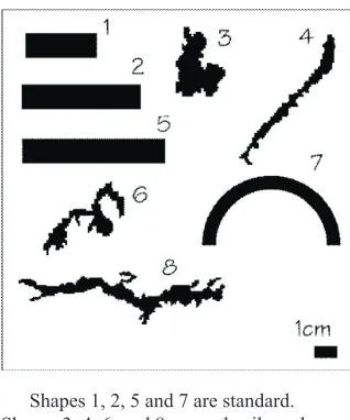
Standard and real pore shapes were combined in Fig. 3 in order to test the equations presented herein, for the calculation of the width and length of such objects as pores of elongated shape. Thus, Fig. 3 is constituted by elongated geometrical shapes, with well-known length and width, which works as standard shapes, and real soil crack shapes.

The real and calculated values of the length and width of the standard and real shapes of soil pores are presented in Table 2. Diference between them and ratio between diffe-rence and real measures), the length and width values of every shape presented in Fig. 3 are calculated from the formulas previously proposed. From the analysis of the results presented in Table 2, it can be verified that the differences and the ratios between the real and the standard values of the length and width, or those calculated from the proposed equations, are very small. The ratio is always less than 3, which is acceptable according to Skeivalas et al.

Shapes 1, 2, 5 and 7 are standard. Shapes 3, 4, 6, and 8 are real soil cracks.

Fig. 3.Standard shapes combined with real soil cracks and irre-gular shapes.

Number Length (cm) Predominant width (cm)

Real Calc. Differ. Ratio Real Calc. Differ. Ratio

1 3.00 2.99 0.01 0.003 1.00 1.01 0.99 0.99

2 6.00 5.97 0.03 0.005 1.00 1.01 0.99 0.99

3 6.11 6.03 0.08 0.000 0.66 0.67 0.01 0.02

4 9.33 9.24 0.09 0.009 0.33 0.33 0.00 0.00

5 7.00 6.96 0.04 0.006 1.00 1.01 0.99 0.99

6 9.91 9.87 0.04 0.004 0.35 0.35 0.00 0.00

7 9.00 8.95 0.05 0.006 0.66 0.67 0.01 0.02

8 17.69 17.58 0.11 0.006 0.36 0.36 0.00 0.00

(8)

(2006). Thus, since it is not easy to evaluate the real values of the length and width of soil cracks, those can be measured through the use of the already mentioned equations, with the certainty of obtaining results that are different from those obtained with the method recommended by Hubertet al. (2007), but much closer to the real values.

It may also be noted that the real length of the forms is always slightly larger than the calculated value, while the width is always slightly smaller than or equal to the calcu-lated value.

CONCLUSIONS

1. TheRvalues are a valuable image analysis tool for defining the separation between shape types, but in some cases they may be not enough.

2. In order to improve the recognition and the classification of soil pores by their shape, based on images from horizontal cross-sections, the values of the following variables should be used, complementarily:Rshape factor, major and minor axes according to the respective procedures provided herein.

3. In horizontal soil cross-section images, Feret’s dia-meter is an acceptable evaluation of the soil biopores dimen-sion. From the values of this variable, biopore classes can be created, corresponding to biopores of different sizes.

4. The length and width of cracks with complex shape and irregular thickness in horizontal soil cross-sections ima-ges are not easily evaluated from image analysis that only furnishes the area, perimeter, major and minor axes, andR shape factor. However, it might be calculated through the insertion of a formula in a calculation sheet.

5. For the calculation of the length of cracks with com-plex shapes, the equation proposed in this work furnishes validated results, close enough to the real values so that they can be used to evaluate this characteristic.

6. For the calculation of the width of the cracks with irre-gular thickness, the formula proposed in this work furnishes validated results, close enough to the real values so that they can be used to evaluate this characteristic.

7. Based on the values of these two variables, crack classes can be created as a function of their width and length. 8. The present study provides a more sensitive image analysis tool for assessing many effects of agricultural managements on the soil structure than the other models. The improved morphometric method presented here, for the study of soil poroids contributes toward the normalization of the image analysis techniques and allows studies to be quicker, more rigorous and accurate, with a perfectly acceptable error ratio.

REFERENCES

Anderson A.N, Crawford J.W., and McBratney A.B., 2000.On diffusion in fractal soil structures. Soil Sci. Soc. Am. J., 4, 24-29.

Bacchi O.O.S., Reichardt K., and Villa Nova N.A., 1996.Fractal scaling of particle and pore size distributions and its relation to soil hydraulic conductivity. Scientia Agricola, 53, 1-6. Bird N.R.A., Perrier E., and Rieu M., 2000.Thewater retention

funtion for a model of soil structure with pore and solid fractal distributions. Eur. J. Soil Sci., 51, 55-63.

Bouma J.A., Jongerius A., Boersma O., Jager A., and Schoon-derbeek E.D., 1977. The function of different types of macropores during saturated flow through four swelling soil horizons. Soil Sci. Soc. Am. J., 41, 945-950.

Bullock P. and Thomasson A.J., 1979.Rothamsted studies of soil structure II. Measurement and characterization of macro-porosity by image analysis and comparison with data from water retention measurements. J. Soil Sci., 30, 391-413. Caniego F.J., Martin M.A., and San Jose F., 2003.Rényi dimensions

of soil pore size distribution. Pedometrics, 112, 205-216. Conway J., 1980.The nature of void spaces in soils of the Salop

and related series. Ph.D. Thesis, University of Wales, Cardiff, UK.

Coomans D. and Massart D.L., 1981.Potential methods in pat-tern recognition. Part I. Classification aspects of the super-vised method ALLOC. Analytica Chimica Acta, 133, 215-250.

Coster M. and Chermant J.L., 1989.Précis d’analyse d’images. CNRS Press, Paris, France.

Cousin I., Porion P., Renault P., and Levitz P., 1999.Gas dif-fusion in a silty-clay soil: experimental study on an undistur-bed soil core and simulation in its three-dimensional recon-struction. Eur. J. Soil Sci., 50, 249-259.

Cox E.P., 1927.A method for assigning numerical and percentage values to the degree of roundness. J. Palaeontology, 1, 179-183. Dagnelis P., 1973.Statistics – Theory and Methods (in Portuguese).

Europa-America Press, Lisbon, Portugal.

Duff M.J.B., 1977. Pattern recognition. Sci. Progress, 64, 423-445.

Holden N.M., 1993.A two-dimensional quantification of soil ped shape. J. Soil Sci., 44, 209-219.

Hubert F., Hallaire V., Sardini P., Caner L., and Heddadj D., 2007. Pore morphology changes under tillage and no-tillage prac-tices. Geoderma,142, 226-236.

Jandel Corporation, Sigma Scan Pro – 4.0 version – Automated Image Analysis Software (User’s manual),1996.CA, USA. Lamandé M., Hallaire V., Curmi P., Peres G., and Cluzeau, D.,

2003.Changes of pore morphology, infiltration and earth-worm community in a silty soil under different agricultural managements. Catena, 54, 637-649.

Lantuejoul C. and Maisonneuve F., 1984.Geodesic methods in quantitative image analysis. Pattern Recognition, 17-2, 177-187.

(9)

Mermut A.R., Grevers M. C. J., and Jong E., 1992.Evaluation of pores under different management systems by image ana-lysis of clay soils in Saskatchewan, Canada. Geoderma, 53, 357-372.

Michell J., 2005.The logic of measurement: A realistic overview. Measurement, 38, 285-294.

Moldrup P., Olesen T., Gamst J., Schjonning P., Yamaguchi T., and Rolston D.E., 2000.Predicting the gas diffusion coefficient in repacked soil: water-induced linear reduction model. Soil Sci. Soc. Am. J., 4, 1588-1594.

Moreau E., Velde B., and. Terribile F, 1999.Comparison of 2D and 3D images of fractures in a Vertisol. Geoderma, 92, 55-72.

Murphy C.P., Bullock P., andBiswell K.J.,1977a.The measu-rement and characterization of voids in thin sections by ima-ge analysis. Part II. Applications. J. Soil Sci., 28, 509-518. Murphy C.P., Bullock P., and Turner R.H., 1977b.The

measu-rement and characterization of voids in soil thin sections by image analysis. Part I. Principles and Techniques. J. Soil Sci., 28, 498-508.

Nawrath R. and Serra J., 1979a.Quantitative image analysis: applications using sequential transformations. Microsc. Acta, 82, 113-128.

Nawrath R. and Serra J., 1979b.Quantitative image analysis: theory and instrumentation, Microsc. Acta, 82, 101-111.

Pagliai M., Vignozzi N., and Pellegrini S., 2004.Soil structure and the effect of managementpractices. Soil Till. Res., 79, 131-143.

Pettijohn F.J., 1957.Sedimentary Rocks. Harper and Row Press, New York, USA.

Ringrose-Voase A.J. and Bullock P., 1984. The automatic re-cognition and measurement of soil pore types by image analysis and computer program. J. Soil Sci., 35, 673-684. Serra J., 1982.Image Analysis and Mathematical Morphology.

Academic Press, New York, USA.

Skeivalas J., Putrimas R., and Buga A., 2006.Information varia-tion during the measure process.Measurement, 39, 532-535.

Steele A.G. and Douglas R.J., 2006.Simplicity with advanced mathematical tools for metrology and testing. Measurement, 39, 795-807.

Thompson M.L., Singh P., Corak S., and Straszheim W.E., 1992. Cautionary notes for the automated analysis of soil pore-space images. Geoderma, 53, 399-415.

USAE, DPLOT - 1.2.0.5 version - (Help and Release Notes),1996. Waterways Experiment Station – Structures Laboratory, Vicksbury, MS, USA.