The Thirty-Third AAAI Conference on Artificial Intelligence (AAAI-19)
Efficient Gaussian Process Classification Using P´olya-Gamma Data Augmentation
Florian Wenzel,
1,*Th´eo Galy-Fajou,
2,*Christan Donner,
2Marius Kloft,
1,3Manfred Opper
2*Contributed equally,1TU Kaiserslautern, Germany,2TU Berlin, Germany,3University of Southern California, USA
[email protected], [email protected], [email protected], [email protected], [email protected]
Abstract
We propose a scalable stochastic variational approach to GP classification building on P´olya-Gamma data augmentation and inducing points. Unlike former approaches, we obtain closed-form updates based on natural gradients that lead to ef-ficient optimization. We evaluate the algorithm on real-world datasets containing up to 11 million data points and demon-strate that it is up to two orders of magnitude faster than the state-of-the-art while being competitive in terms of prediction performance.
1
Introduction
Gaussian processes (GPs) (Rasmussen and Williams 2005) provide a popular Bayesian non-linear non-parametric method for regression and classification. Because of their ability of accurately adapting to data and thus achieving high prediction accuracy while providing well calibrated uncer-tainty estimates, GPs are a standard method in several appli-cation areas, including geospatial predictive modeling (Stein 2012) and robotics (Dragiev, Toussaint, and Gienger 2011).
However, recent trends in data availability in the sciences and technology have made it necessary to develop algo-rithms capable of processing massive data (John Walker 2014). Currently, GP classification has limited applicabil-ity to big data. Naive inference typically scales cubic in the number of data points, and exact computation of posterior and marginal likelihood is intractable.
Nevertheless, the combination of so-called sparse Gaus-sian process techniques with approximate inference meth-ods, such as expectation propagation (EP) or the varia-tional approach, have enabled GP classification for datasets containing millions of data points (Hern´andez-Lobato and Hern´andez-Lobato 2016; Salimbeni, Eleftheriadis, and Hensman 2018).
While these results are already impressive, we will show in this paper that a speedup of up to two orders magni-tudes can be achieved. Our approach is based on consid-ering an augmented version of the original GP classifica-tion model and replacing the ordinary (stochastic) gradients for optimization by more efficientnatural gradients, which
Copyright c2019, Association for the Advancement of Artificial Intelligence (www.aaai.org). All rights reserved.
is the standard Euclidean gradient multiplied by the in-verse Fisher information matrix. Natural gradients recently have been successfully used in a variety of variational in-ference problems (Honkela et al. 2010; Wenzel et al. 2017; J¨ahnichen et al. 2018).
Unfortunately, an efficient computation of the natural gra-dient for the GP classification problem is not straight for-ward. The use of the probit link function in Dezfouli and Bonilla (2015); Hern´andez-Lobato and Hern´andez-Lobato (2016); Mandt et al. (2017); Salimbeni, Eleftheriadis, and Hensman (2018) leads to expectations in the variational ob-jective functions that can only be computed by numerical quadrature, thus, preventing efficient optimization.
We derive a natural-gradient approach to variational in-ference in GP classification based on thelogitlink. We ex-ploit that the corresponding likelihood has an auxiliary vari-able representation as a continuous mixture of Gaussians in-volving P´olya-Gamma random variables (Polson, Scott, and Windle 2013).
Unlike former approaches, our natural gradient updates can be computed in closed-form. Moreover, they have the advantage that they correspond to block-coordinate ascent updates and, therefore, learning rates close to one can be chosen. This leads to a fast and stable algorithm which is simple to implement. Our main contributions are as follows:
• We present a Gaussian process classification model using a logit link function that is based on P´olya-Gamma data augmentation and inducing points for Gaussian process inference.
• We derive an efficient inference algorithm based on stochastic variational inference and natural gradients. All natural gradient updates are given in closed-form and do not rely on numerical quadrature methods or sampling ap-proaches. Natural gradients have the advantage that they provide effective second-order optimization updates.
• In our experiments, we demonstrate that our approach drastically improves speed up to two orders of magni-tude while being competitive in terms of prediction per-formance. We apply our method to massive real-world datasets up to 11 million points and demonstrate superior scalability.
GP classification model and in section 4 we present an ef-ficient variational inference algorithm. Section 5 concludes with experiments. Our code is available via Github1.
2
Background and Related Work
Gaussian process classification Hensman and Matthews (2015) consider Gaussian process classification with a pro-bit inverse link function and suggest a variational Gaussian model that builds on inducing points. By employing auto-matic differentiation, Salimbeni, Eleftheriadis, and Hens-man (2018) generalize this approach to use natural gradients in non-conjugate GP models. Khan and Nielsen (2018) con-sider natural gradient updates in the setting of variational inference with exponential families. Unlike our approach, these methods do not benefit from closed-form updates and have to resort to numerical approximations. Moreover, our approach has the advantage that a higher learning rate close to one can be chosen leading to updates that can be inter-preted as block-coordinate ascent updates.
Izmailov, Novikov, and Kropotov (2018) use tensor train decomposition to allow for the training of GP models with billions of inducing points. The updates are not computed in closed-form and they do not use natural gradients.
Dezfouli and Bonilla (2015) propose a general automated variational inference approach for sparse GP models with non-conjugate likelihood. Since they follow a black box ap-proach and do not exploit model specific properties they do not employ efficient optimization techniques.
Hern´andez-Lobato and Hern´andez-Lobato (2016) follow an expectation propagation approach based on inducing points and have a similar computational cost as Hensman and Matthews (2015).
P´olya-Gamma data augmentation Polson, Scott, and Windle (2013) introduced the idea of data augmentation in logistic models using the class of P´olya-Gamma distribu-tions. This allows for exact inference via Gibbs sampling or approximate variational inference schemes (Scott and Sun 2013).
Linderman, Johnson, and Adams (2015) extend this idea to multinomial models and discuss the application for Gaus-sian processes with multinomial observations but their ap-proach does not scale to big datasets and they do not con-sider the concept of inducing points.
3
Model
The logit GP Classification model is defined as follows. Let
X = (x1, . . . ,xn) ∈ Rd×n be thed-dimensional training
points with labelsy= (y1, . . . , yn)∈ {−1,1}n. The
likeli-hood of the labels is
p(y|f, X) =
n
Y
i=1
σ(yif(xi)), (1)
whereσ(z) = (1 + exp(−z))−1 is the logit link function
andf is the latent decision function. We place a GP prior
1
https://github.com/theogf/AugmentedGaussianProcesses.jl
overf and obtain the joint distribution of the labels and the latent GP
p(y,f|X) =p(y|f, X)p(f|X), (2)
wherep(f|X) =N(f|0, Knn)andKnndenotes the kernel
matrix evaluated at the training points X. For the sake of clarity we omit the conditioning onX in the following.
3.1
P´olya-Gamma data augmentation
Due to the analytically inconvenient form of the likelihood function, inference for logit GP classification is a challeng-ing problem. We aim to remedy this issue by considerchalleng-ing an augmented representation of the original model. Later we will see that the augmented model is indeed advantageous as it leads to efficient closed-form updates in our variational inference scheme.
Polson, Scott, and Windle (2013) introduced the class of P´olya-Gamma random variables and proposed a data aug-mentation strategy for inference in models with binomial likelihoods. The augmented model has the appealing prop-erty that the likelihood of the latent functionf is propor-tional to a Gaussian density when conditioned on the aug-mented P´olya-Gamma variables. This allows for Gibbs sam-pling methods, where model parameters and P´olya-Gamma variables can be sampled alternately from the posterior (Pol-son, Scott, and Windle 2013). Alternatively, the augmenta-tion scheme can be utilized to derive an efficient approxi-mate inference algorithm in the variational inference frame-work, which will be pursued here.
The P´olya-Gamma distribution is defined as follows. The random variable ω ∼ PG(b,0),b > 0 is defined by the moment generating function
EPG(ω|b,0)[exp(−ωt)] =
1
coshb(pt/2). (3)
It can be shown that this is the Laplace transform of an in-finite convolution of gamma distributions. The definition is related to our problem by the fact that the logit link can be written in a form that involves the cosh function, namely
σ(zi) = exp(12zi)(2 cosh(z2i))−1. In the following we
de-rive a representation of the logit link in terms of P´olya-Gamma variables.
First, we define the generalPG(b, c)class which is de-rived by an exponential tilting of thePG(b,0)density, it is given by
PG(ω|b, c)∝exp(−c 2
2ω)PG(ω|b,0).
From the moment generating function (3) the first moment can be directly computed
EP G(ω|b,c)[ω] =
b
2ctanh
c 2
.
For the subsequently presented variational algorithm these properties suffice and the full representation of the P´olya-Gamma densityPG(ω|b, c)is not required.
do this we write the non-conjugate logistic likelihood func-tion (1) in terms of P´olya-Gamma variables
σ(zi) = (1 + exp(−zi))− 1
= exp(
1 2zi)
2 cosh(zi
2)
=1 2
Z exp
z
i
2 −
z2 i
2 ωi
p(ωi)dωi, (4)
wherep(ωi) = PG(ωi|1,0)and by making use of (3). For
more details see Polson, Scott, and Windle (2013). Using this identity and substitutingzi =yif(xi)we augment the
joint density (2) with P´olya-Gamma variables
p(y,ω,f)∝exp 1
2y >f −1
2f
>Ωfp(f)p(ω), (5)
whereΩ = diag(ω) is the diagonal matrix of the P´olya-Gamma variables{ωi}. In contrast to the original model (2) the augmented model is conditionally conjugate forming the basis for deriving closed-form updates in section 4.
Interestingly, employing a structured mean-field varia-tional inference approach (cf. section 4) to the plain P´olya-Gamma augmented model (5) leads to the same bound for GP classification derived by Gibbs and MacKay (2000). This is an interesting new perspective on this bound since they do not employ a data augmentation approach. We pro-vide a proof in appendix A.5. Our approach goes beyond Gibbs and MacKay (2000) by providing a fully Bayesian perspective, including a sparse GP prior (section 3.2) in the model and proposing a scalable inference algorithm based on natural gradients (section 4).
3.2
Sparse Gaussian process
Inference in GP models typically has the computational complexityO(n3). We obtain a scalable approximation of
our model and focus on inducing point methods (Snelson and Ghahramani 2006). We follow a similar approach as in Hensman and Matthews (2015) and reduce the complexity toO(m3), wheremis number of inducing points.
We augment the latent GP f withm additional input-output pairs(Z1, u1), . . . ,(Zm, um), termed asinducing
in-putsandinducing variables. The function values of the GPf
and the inducing variablesu= (u1, . . . , um)are connected
via
p(f|u) =Nf|KnmKmm−1 u,Ke
p(u) =N(u|0, Kmm),
(6)
whereKmm is the kernel matrix resulting from evaluating
the kernel function between all inducing inputs, Knm is
the cross-kernel matrix between inducing inputs and train-ing points andKe =Knn−KnmKmm−1 Kmn. Including the
inducing points in our model gives the augmented joint dis-tribution
p(y,ω,f,u) =p(y|ω,f)p(ω)p(f|u)p(u) (7)
Note that the original model (2) can be recovered by marginalizingωandu.
4
Inference
The goal of Bayesian inference is to compute the poste-rior of the latent model variables. Because this problem is intractable for the model at hand, we employ variational inference to map the inference problem to a feasible op-timization problem. We first chose a family of tractable variational distributions and select the best candidate by minimizing the Kullback-Leibler divergence between the variational distribution and the posterior. This is equivalent to optimizing a lower bound on the marginal likelihood, known as evidence lower bound (ELBO) (Jordan et al. 1999; Wainwright and Jordan 2008).
In the following we develop a stochastic variational in-ference (SVI) algorithm that enables stochastic optimization based on natural gradient updates which are given in closed-form.
4.1
Why use natural gradients?
Using the natural gradient over the standard Euclidean gradi-ent is favorable since natural gradigradi-ents are invariant to repa-rameterization of the variational family (Amari and Nagaoka 2007; Martens 2017) and provide effective second-order op-timization updates (Amari 1998; Hoffman et al. 2013).
The superiority of using natural gradients in our approach can be explained by the following. We reformulate the GP classification model as an augmented model which is con-ditionally conjugate. When using a learning rate of one, the natural gradient updates correspond to block-coordinate as-cent updates, i.e. in each iteration each parameter is set to its optimal value given the remaining parameters (see ap-pendix A.4 and Hoffman et al. (2013)). In practice, we em-ploy stochastic variational inference, i.e. we only use mini-batches of the data to obtain a noisy version of the natural gradient. In this setting, learning rates slightly less than one have to be chosen.
This is in contrast to former natural gradient based approaches, e.g. (Salimbeni, Eleftheriadis, and Hensman 2018), that focus on the original non-conjugate GP clas-sification model. Although they benefit from using natural gradients, they have the disadvantage that their updates do not correspond to coordinate-ascent updates. Thus, learning rates that are much smaller that one have to be used to assure convergence.
Therefore, in our approach, we can use much higher learn-ing rates and optimization is faster and more stable which we demonstrate in the experiments.
4.2
Variational approximation
We aim to approximate the posterior of the inducing points p(u|y) and apply the methodology of variational inference to the marginal joint distribution p(y, ω, u) =
p(y|ω,u)p(ω)p(u). Following a similar approach as Hens-man and Matthews (2015), we apply Jensen’s inequality to obtain a tractable lower bound on the log-likelihood of the labels
logp(y|ω,u) = logEp(f|u)[p(y|ω, f)]
By this inequality we construct a variational lower bound on the evidence
logp(y)≥Eq(u,ω)[logp(y|u,ω)]−KL (q(u,ω)||p(u,ω))
≥Ep(f|u)q(u)q(ω)[logp(y|ω,f)]
−KL (q(u,ω)||p(u,ω)) =:L,
where the first inequality is the usual evidence lower bound (ELBO) in variational inference and the second inequality is due to (8).
We follow a structured mean-field approach (Wainwright and Jordan 2008) and assume independence between the in-ducing variablesuand P´olya-Gamma variablesω, yielding a variational distribution of the formq(u, ω) = q(u)q(ω). Setting the functional derivative ofLw.r.t.q(u)andq(ω)to zero, respectively, results in the following consistency con-dition for the maximum,
q(u,ω) =q(u)Y
i
q(ωi), (9)
withq(ωi) = PG(ωi|1, ci)andq(u) = N(u|µ,Σ).
Re-markably, we do not have to use the full P´olya-Gamma classPG(ωi|bi, ci), but instead consider the restricted class
bi = 1since it already contains the optimal distribution.
We use (9) as variational family which is parameterized by the variational parameters{µ,Σ,c}and obtain a closed-form expression of the variational bound
L(c,µ,Σ)
=Ep(f|u)q(u)q(ω)[logp(y|ω,f)]−KL (q(u,ω)||p(u,ω))
c
=1 2
log|Σ| −log|Kmm|)−tr(Kmm−1 Σ)−µ>Kmm−1µ
+X
i
n
yiκiµ−θi
e
Kii−κiΣκ>i −µ >
κ>iκiµ
+c2iθi−2 logcosh ci
2 o
, (10)
where θi = 2c1itanh c2i
and κi = KimKmm−1 .
Re-markably, all intractable terms involving expectations of log PG(ωi|1,0)cancel out. Details are provided in appendix A.2.
4.3
Stochastic variational inference
Our algorithm alternates between updates of the local varia-tional parameterscand global parametersµandΣ. In each iteration we update the parameters based on a mini-batch of the dataS ⊂ {1, ..., n}of sizes=|S|.
We update thelocal parameterscSin the mini-batchSby employing coordinate ascent. To this end, we fix the global parameters and analytically compute the unique maximum of (10) w.r.t. the local parameters, leading to the updates
ci=
q
e
Kii+κiΣκ>i +µ>κ>i κiµ (11)
fori∈ S.
We update theglobal parametersby employing stochastic optimization of the variational bound (10). The optimization is based on stochastic estimates of the natural gradients of the global parameters. We use the natural parameterization
of the variational Gaussian distribution, i.e., the parameters η1:= Σ−1µandη
2 =−12Σ−1. Using the natural
parame-ters results in simpler and more effective updates. The natu-ral gradients based on the mini-batchSare given by
e
∇η1LS =
n
2sκ
>
SyS−η1
e
∇η2LS =− 1 2
Kmm−1 +n
sκ
> SΘSκS
−η2,
(12)
whereΘ =diag(θ)andθi= 2c1itanh
ci
2
. The factorns is due to the rescaling of the mini-batches. The global param-eters are updated according to a stochastic natural gradient ascent scheme. We employ the adaptive learning rate method described by Ranganath et al. (2013).
The natural gradient updates always lead to a positive def-inite covariance matrix2 and in contrast to Hensman and
Matthews (2015) our implementation does not require any assurance for positive-definiteness of the variational covari-ance matrixΣ. Details for the derivation of the updates can be found in appendix A.3. The complexity of each iteration in the inference scheme isO(m3), due to the inversion of
the matrixη2.
On the quality of the approximation In other applica-tions of variational inference to GP classification, one tries to approximate the posterior directly by a Gaussianq∗(f) which minimizes the Kullback-Leibler divergence between the variational distribution and the true posterior (Hensman and Matthews 2015). On the other hand, in our paper, we apply variational inference to the augmented model, looking for the best distribution that factorizes in the P´olya-Gamma variablesωiand the original functionf. This approach also
yields a Gaussian approximationq(f)as a factor in the op-timal density. Of courseq(f)will be different from the ‘op-timal’q∗(f). We could however argue that asymptotically, in the limit of a large number of data, the predictions given by both densities may not be too different, as the posterior uncertainty for both densities should become small (Opper and Archambeau 2009).
It would be interesting to see how the ELBOs of the two variational approaches, which both give a lower bound on the likelihood of the data, differ. Unfortunately, such a com-putation would require the knowledge of the optimalq∗(f). However, we can obtain some estimate of this difference when we assume that we use thesameGaussian densityq(f) for both bounds as an approximation. In this case, we obtain
Lorig− Laugmented=Eq(f)[KL(q(ω)||p(ω|f, y))].
This lower bound on the gap is small if on average the varia-tional approximationq(ω)is close to the posteriorp(ω|f, y). For the sake of simplicity we consider here the non-sparse case, i.e. the inducing points equal the training points (f =
u). However, it is straight-forward to extend the results also to the sparse case.
We empirically investigate the quality of our approxima-tion in experiment 5.1.
2
Predictions The approximate posterior of the GP values and inducing variables is given byq(f,u) = p(f|u)q(u), whereq(u) = N(u|µ,Σ)denotes the optimal variational distribution. To predict the latent function valuesf∗at a test point x∗ we substitute our approximate posterior into the standard predictive distribution
p(f∗|y) = Z
p(f∗|f,u)p(f,u|y)dfdu
≈
Z
p(f∗|f,u)p(f|u)q(u)dfdu
= Z
p(f∗|u)q(u)du=N f∗|µ∗, σ∗2
, (13)
where the prediction mean is µ∗ = K∗mKmm−1 µand the
variance σ2
∗ = K∗∗+K∗mKmm−1(ΣKmm−1 −I)Km∗. The matrixK∗mdenotes the kernel matrix between the test point
and the inducing points andK∗∗the kernel value of the test point. The distribution of the test labels is easily computed by applying the logit link function to (13),
p(y∗= 1|y) = Z
σ(f∗)p(f∗|y)df∗. (14)
This integral is analytically intractable but can be computed numerically by quadrature methods. This is adequate and fast since the integral is only one-dimensional.
Computing the mean and the variance of the predictive distribution has complexityO(m)andO(m2), respectively.
Optimization of the hyperparameters We select the op-timal kernel hyperparameters by maximizing the marginal likelihoodp(y|h), wherehdenotes the set of hyperparam-eters (this approach is called empirical Bayes (Maritz and Lwin 1989)). We follow an approximate approach and opti-mize the fitted variational lower boundL(h)(10) as a func-tion of h by alternating between optimization steps w.r.t. the variational parameters and the hyperparameters (Mandt, Hoffman, and Blei 2016).
5
Experiments
We compare our proposed method, efficient Gaussian pro-cess classification (X-GPC), with the state-of-the-art meth-odsSVGPC(Salimbeni, Eleftheriadis, and Hensman 2018), provided in the package GPflow3 (Matthews et al. 2017),
which builds on TensorFlow and the EP approach EPGPC by Hern´andez-Lobato and Hern´andez-Lobato (2016), imple-mented in R. All methods are applied to real-world datasets containing up to 11 million data points.
In all experiments a squared exponential covariance func-tion with a common length scale parameter for each dimen-sion, an amplitude parameter and an additive noise param-eter is used. The kernel hyperparamparam-eters are initialized to the same values and optimized using Adam (Kingma and Ba 2014), while inducing points location are initialized via k-means++ (Arthur and Vassilvitskii 2007) and kept fixed during training. The SVI based methods,X-GPCandSVGPC,
3
We use GPflow version 1.2.0.
Figure 1: Posterior mean (µ), variance (σ) and predictive marginals (p) of the Diabetes dataset. Each plot shows the MCMC ground truth on the x-axis and the estimated value of our model on the y-axis. Our approximation is very close to the ground truth.
use an adaptive learning rate. All algorithms are run on a sin-gle CPU. We experiment on 12 datasets from the OpenML website and the UCI repository ranging from 768 to 11 mil-lion data points. In the first experiment (section 5.1), we ex-amine the quality of the approximation provided byX-GPC. In the next experiment, we evaluate the prediction perfor-mance and run time of X-GPCand SVGPC and EPGPC on several real-world datasets. Finally, in 5.3, we examine the sensitivity of all methods to the number of inducing points.
5.1
Quality of the approximation
We empirically examine the quality of the variational ap-proximation provided by our method. In Fig. 1, we com-pare the approximations to the true posterior obtained by employing an asymptotically correct Gibbs sampler (Polson and Scott 2011; Linderman, Johnson, and Adams 2015). We compare the posterior mean and variance as well as the pre-diction probabilities with the ground truth. Since the Gibbs sampler does not scale to large datasets we experiment on the small Diabetes dataset. In Fig. 1 we plot the mated values vs. the ground truth. We find that our approxi-mation is very close to the true posterior.
5.2
Numerical comparison
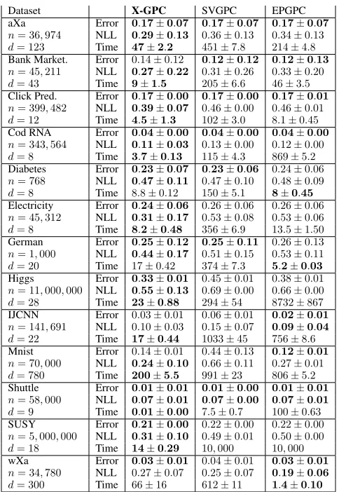
We evaluate the prediction performance and run time of our methodX-GPCand the competing methodsSVGPCand EPGPC. We experiment on a variety of different datasets and report the resulting prediction error, negative test log-likelihood and run time for each method in table 1.
The experiments are conducted as follows. For each dataset we perform a 10-fold cross-validation and for datasets with more than 1 million points, we limit the test set to 100,000 points. We report the average prediction er-ror, the negative test log-likelihood (14) and the run time along with one standard deviation. For all datasets, we use 100 inducing points and a mini-batch size of 100 points.
For X-GPC we find that the following simple conver-gence criterion on the global parameters leads to good re-sults: a sliding window average being smaller than a thresh-old of 10−4 . Unfortunately, the original implementations
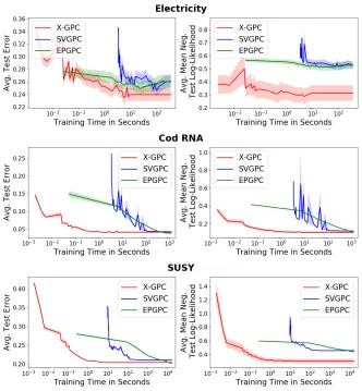
Figure 2: Average negative test log-likelihood and average test prediction error as a function of training time (seconds in alog10 scale) on the datasets Electricity (45,312 points), Cod RNA (343,564 points) and SUSY (5 million points).X-GPC(proposed) reaches values close to the optimum after only a few iterations, whereasSVGPCandEPGPCare one to two orders of magnitude slower.
Dataset X-GPC SVGPC EPGPC aXa Error 0.17±0.07 0.17±0.07 0.17±0.07
n= 36,974 NLL 0.29±0.13 0.36±0.13 0.34±0.13
d= 123 Time 47±2.2 451±7.8 214±4.8
Bank Market. Error 0.14±0.12 0.12±0.12 0.12±0.13
n= 45,211 NLL 0.27±0.22 0.31±0.26 0.33±0.20
d= 43 Time 9±1.5 205±6.6 46±3.5
Click Pred. Error 0.17±0.00 0.17±0.00 0.17±0.01
n= 399,482 NLL 0.39±0.07 0.46±0.00 0.46±0.01
d= 12 Time 4.5±1.3 102±3.0 8.1±0.45
Cod RNA Error 0.04±0.00 0.04±0.00 0.04±0.00
n= 343,564 NLL 0.11±0.03 0.13±0.00 0.12±0.00
d= 8 Time 3.7±0.13 115±4.3 869±5.2
Diabetes Error 0.23±0.07 0.23±0.06 0.24±0.06
n= 768 NLL 0.47±0.11 0.47±0.10 0.48±0.09
d= 8 Time 8.8±0.12 150±5.1 8±0.45 Electricity Error 0.24±0.06 0.26±0.06 0.26±0.06
n= 45,312 NLL 0.31±0.17 0.53±0.08 0.53±0.06
d= 8 Time 8.2±0.48 356±6.9 13.5±1.50
German Error 0.25±0.12 0.25±0.11 0.26±0.13
n= 1,000 NLL 0.44±0.17 0.51±0.15 0.53±0.11
d= 20 Time 17±0.42 374±7.3 5.2±0.03 Higgs Error 0.33±0.01 0.45±0.01 0.38±0.01
n= 11,000,000 NLL 0.55±0.13 0.69±0.00 0.66±0.00
d= 28 Time 23±0.88 294±54 8732±867
IJCNN Error 0.03±0.01 0.06±0.01 0.02±0.01
n= 141,691 NLL 0.10±0.03 0.15±0.07 0.09±0.04
d= 22 Time 17±0.44 1033±45 756±8.6
Mnist Error 0.14±0.01 0.44±0.13 0.12±0.01
n= 70,000 NLL 0.24±0.10 0.66±0.11 0.27±0.01
d= 780 Time 200±5.5 991±23 806±5.2
Shuttle Error 0.01±0.01 0.01±0.00 0.01±0.01
n= 58,000 NLL 0.07±0.01 0.07±0.00 0.07±0.01
d= 9 Time 0.01±0.00 7.5±0.7 100±0.63
SUSY Error 0.21±0.00 0.22±0.00 0.22±0.00
n= 5,000,000 NLL 0.31±0.10 0.49±0.01 0.50±0.00
d= 18 Time 14±0.29 10,000 10,000
wXa Error 0.03±0.01 0.04±0.01 0.03±0.01
n= 34,780 NLL 0.27±0.07 0.25±0.07 0.19±0.06
d= 300 Time 66±16 612±11 1.4±0.10
Table 1: Average test prediction error, negative test log-likelihood (NLL) and time in seconds along with one stan-dard deviation. Best values are highlighted.
a fair comparison, we therefore monitor the convergence of the prediction performance on a hold-out set and use a slid-ing window average of size 5 and threshold10−3as
conver-gence criterion for all methods.
We observe thatX-GPCis about one to two orders of mag-nitude faster thanSVGPCandEPGPCon most datasets. Only on the dataset wXa,EPGPCis slightly faster thanX-GPC. The prediction error is similar for all methods butX-GPC outper-forms the competitors in terms of the test log-likelihood on most datasets (aXa, Bank Marketing, Click Prediction, Cod RNA, Diabetes, Electricity, German, Higgs, Mnist, SUSY). This means that the confidence levels in the predictions are better calibrated for X-GPC, i.e. when predicting a wrong labelSVGPCandEPGPCtend to be more confident than X-GPC.
Performance as a function of time Since all considered methods are based on an optimization schemes, there is a trade-off between the run time of the algorithm and the pre-diction performance. We make this trade-off transparent by plotting the prediction performance as function of time on
each dataset. For each method we monitor on a 10-fold cross-validation the average negative test log-likelihood and prediction error on a hold-out test set as a function of time.
The results are displayed in Fig. 2 for three selected datasets, while the results for the remaining datasets are de-ferred to appendix A.1. For all datasets we observe that after a few iterationsX-GPCis already close to the optimum due to its efficient closed form natural gradient updates. Both the prediction error and test log-likelihood converge around one to two orders of magnitude faster for X-GPCthan for SVGPCandEPGPC. Moreover, the performance curves tend to be noisier forSVGPCthan forX-GPCandEPGPC. For the datasets HIGGS and IJCNN, EPGPClead to slightly better final prediction performance, but with the cost of a runtime being up to 4 orders of magnitude slower thanX-GPC (ap-prox. 28 hours vs. 9 and 435 seconds, respectively).
All three methods are implemented in different program-ming frameworks: X-GPC in Julia, SVGPC in TensorFlow and EPGPC in R leading to different efficient implemen-tations. However, we find that the main speed-up of our method is due to the efficient natural gradient updates and only marginally related to the usage of a different program-ming language. To check this we implementedEPGPCalso in Julia and obtained similar runtimes. SinceSVGPCis part of the highly optimized GPflow package we only used the original implementation.
5.3
Inducing points
We examine the effect of different numbers of inducing points on the prediction performance and run time. For all methods we compare different numbers of inducing points:
M = 16,32,64,128. For each setting, we perform a 10-fold cross validation on the Shuttle dataset and plot the mean pre-diction error as function of time. The results are displayed in Fig. 3. We observe that the higher the number of inducing points, the better the prediction performance, but the longer the run time. Throughout all settings of inducing points our method is consistently faster of around one to two orders of magnitude than the competitors. On the Shuttle dataset us-ing onlyM = 32inducing points is enough and can only be marginally improved by using more inducing point for all methods. However, the performance curves of SVGPC are instable when using less than 128 inducing points.
6
Conclusions
We proposed an efficient Gaussian process classification method that builds on P´olya-Gamma data augmentation and inducing points. The experimental evaluations shows that our method is up to two orders of magnitude faster than the state-of-the-art approach while being competitive in terms of prediction performance. Speed improvements are due to the P´olya-Gamma data augmentation approach that enables efficient second order optimization.
may aim at extending the approach to class and multi-label classification.
Acknowledgements We thank Stephan Mandt, James Hensman and Scott W. Linderman for fruitful discussions. This work was partly funded by the German Research Foun-dation (DFG) awards KL 2698/2-1 and GRK1589/2 and the by the Federal Ministry of Science and Education (BMBF) awards 031L0023A, 01IS18051A.
References
Amari, S., and Nagaoka, H. 2007.Methods of Information Geom-etry. American Mathematical Society.
Amari, S. 1998. Natural grad. works efficiently in learning.Neural Computation.
Arthur, D., and Vassilvitskii, S. 2007. k-means++: The advantages of careful seeding. InProceedings of the eighteenth annual ACM-SIAM symposium on Discrete algorithms, 1027–1035. Society for Industrial and Applied Mathematics.
Dezfouli, A., and Bonilla, E. V. 2015. Scalable inference for gaus-sian process models with black-box likelihoods. InNIPS, 1414– 1422.
Dragiev, S.; Toussaint, M.; and Gienger, M. 2011. Gaussian process implicit surfaces for shape estimation and grasping. In Robotics and Automation (ICRA), 2845–2850.
Gibbs, M. N., and MacKay, D. J. C. 2000. Variational Gaus-sian process classifiers. IEEE Transactions on Neural Networks 11(6):1458–1464.
Hensman, J., and Matthews, A. 2015. Scalable Variational Gaus-sian Process Classification. InAISTATS.
Hern´andez-Lobato, D., and Hern´andez-Lobato, J. M. 2016. Scal-able gaussian process classification via expectation propagation. In AISTATS.
Hoffman, M. D.; Blei, D. M.; Wang, C.; and Paisley, J. 2013. Stochastic Variational Inference.Journal of Machine Learning Re-search.
Honkela, A.; Raiko, T.; Kuusela, M.; Tornio, M.; and Karhunen, J. 2010. Approximate riemannian conjugate gradient learning for fixed-form variational bayes. Journal of Machine Learning Re-search11.
Izmailov, P.; Novikov, A.; and Kropotov, D. 2018. Scalable gaus-sian processes with billions of inducing inputs via tensor train de-composition. InAISTATS, 726–735.
J¨ahnichen, P.; Wenzel, F.; Kloft, M.; and Mandt, S. 2018. Scalable generalized dynamic topic models. InAISTATS.
John Walker, S. 2014. Big data: A revolution that will transform how we live, work, and think. Taylor & Francis.
Jordan, M. I.; Ghahramani, Z.; Jaakkola, T. S.; and Saul, L. K. 1999. An Introduction to Variational Methods for Graphical Mod-els.Machine Learning.
Khan, M. E., and Nielsen, D. 2018. Fast yet simple natural-gradient descent for variational inference in complex models.Arxiv Preprint.
Kingma, D. P., and Ba, J. 2014. Adam: A method for stochastic optimization.CoRRabs/1412.6980.
Linderman, S. W.; Johnson, M. J.; and Adams, R. P. 2015. De-pendent multinomial models made easy: Stick-breaking with the polya-gamma augmentation. InNIPS.
Mandt, S.; Wenzel, F.; Nakajima, S.; Cunningham, J. P.; Lippert, C.; and Kloft, M. 2017. Sparse Probit Linear Mixed Model. Ma-chine Learning Journal.
Mandt, S.; Hoffman, M.; and Blei, D. 2016. A Variational Analysis of Stochastic Gradient Algorithms.ICML.
Maritz, J., and Lwin, T. 1989. Empirical Bayes Methods with Applications.Monographs on Statistics and Applied Probability. Martens, J. 2017. New insights and perspectives on the natural gradient method.Arxiv Preprint.
Matthews, A. G. d. G.; van der Wilk, M.; Nickson, T.; Fujii, K.; Boukouvalas, A.; Le´on-Villagr´a, P.; Ghahramani, Z.; and Hens-man, J. 2017. GPflow: A Gaussian process library using Ten-sorFlow.Journal of Machine Learning Research.
Opper, M., and Archambeau, C. 2009. The variational gaussian approximation revisited.Neural Comput.21(3):786–792. Polson, N. G., and Scott, S. L. 2011. Data augmentation for support vector machines.Bayesian Anal.
Polson, N. G.; Scott, J. G.; and Windle, J. 2013. Bayesian inference for logistic models using p´olya–gamma latent variables.Journal of the American Statistical Association108(504):1339–1349. Ranganath, R.; Wang, C.; Blei, D. M.; and Xing, E. P. 2013. An Adaptive Learning Rate for Stochastic Variational Inference. ICML.
Rasmussen, C. E., and Williams, C. K. I. 2005. Gaussian Pro-cesses for Machine Learning (Adaptive Computation and Machine Learning). The MIT Press.
Salimbeni, H.; Eleftheriadis, S.; and Hensman, J. 2018. Natural gradients in practice: Non-conjugate variational inference in gaus-sian process models. InAISTATS.
Scott, J. G., and Sun, L. 2013. Expectation-maximization for lo-gistic regression.arXiv preprint arXiv:1306.0040.
Snelson, E., and Ghahramani, Z. 2006. Sparse GPs using Pseudo-inputs.NIPS.
Stein, M. L. 2012. Interpolation of spatial data: some theory for kriging. Springer Science & Business Media.
Wainwright, M. J., and Jordan, M. I. 2008. Graphical models, ex-ponential families, and variational inference.Found. Trends Mach. Learn.1–305.