Bayesian Deep Collaborative Matrix Factorization

The Thirty-Third AAAI Conference on Artificial Intelligence (AAAI-19)

Bayesian Deep Collaborative Matrix Factorization

Teng Xiao,

Shangsong Liang,

Weizhou Shen,

Zaiqiao Meng

2_{Guangdong Key Laboratory of Big Data Analysis and Processing, Guangzhou 510006, China} {cstengxiao, liangshangsong}@gmail.com, [email protected], [email protected]

Abstract

In this paper, we propose a Bayesian DeepCollaborative

MatrixFactorization (BDCMF) algorithm for collaborative filtering (CF). BDCMF is a novel Bayesian deep generative model that learns user and item latent vectors from users’ social interactions, contents of items as the auxiliary infor-mation and user-item rating (feedback) matrix. It alleviates the problem of matrix sparsity by incorporating items’ auxil-iary and users’ social information into the model. It can learn more robust and dense latent representations by integrating deep learning into Bayesian probabilistic framework. As be-ing one of deep generative models, it has both non-linearity and Bayesian nature. Additionally, in BDCMF, we derive an efficient EM-style point estimation algorithm for parameter learning. To further improve recommendation performance, we also derive a full Bayesian posterior estimation algorithm for inference. Experiments conducted on two sparse datasets show that BDCMF can significantly outperform the state-of-the-art CF methods.

Introduction

Social media, e.g., Facebook and Twitter, has greatly influ-enced people’s daily lives, and thus building an effective Recommender System (RS) for them has attracted many in-terests in recent years. The most used technique in RS is col-laborative filtering (CF), which makes use of users’ ratings over items. Matrix factorization (MF) (Mnih and Salakhut-dinov 2008) is one of the most commonly used CF methods due to its effectiveness and scalability. The goal of MF is to learn latent factors of both users and items from user-item feedback matrix. However, traditional MF methods suffer from the matrix sparsity problem – recommendation perfor-mance drops dramatically when the user-item feedback ma-trix is very sparse. In addition, traditional MF methods as-sume users are independent and identically distributed, and ignore the social connections among users.

To alleviate the matrix sparsity problem, many social MF methods such as those in (Park, Kim, and Choi 2013; Adams, Dahl, and Murray 2014) incorporate auxiliary infor-mation, e.g., content information of items, into MF. How-ever, these methods incorporate auxiliary information as a

∗

Shangsong Liang is the corresponding author.

Copyright c2019, Association for the Advancement of Artificial Intelligence (www.aaai.org). All rights reserved.

linear regularization term, resulting in the fact that learn-ing latent representations of users and items is not effec-tive when the auxiliary information is also sparse. Aiming at learning more effective representations, many CF-based models using different types of auxiliary information, such as latent Dirichlet allocation (LDA) (Wang and Blei 2011), stacked denoising autoencoder (SDAE) (Wang, Wang, and Yeung 2015; Zhang et al. 2016), variational autoencoder(Li and She 2017) and marginalized denoising autoencoder (Li, Kawale, and Fu 2015), have been proposed to obtain items’ latent content representations. Nevertheless, all these mod-els ignore social connections among users.

In order to jointly utilize item contents and social net-work information, some hybrid MF methods have been pro-posed, which can be roughly classified into two categories: i.e., Collaborative Topic Regression (CTR)-based methods (Wang and Blei 2011; Chen et al. 2014; Purushotham, Liu, and Kuo 2012; Wang, Chen, and Li 2013; Xu et al. 2017) and Collaborative Deep Learning (CDL)-based meth-ods (Wang, Wang, and Yeung 2015; Zhang et al. 2016; Nguyen and Lauw 2017). Although CTR-based and CDL-based methods have achieved great performance, the full Bayesian posterior estimation is intractable in these mod-els. All these models need to maximize a point estimation for parameter learning. However, in this paper, we point out that maximizing such a point estimation actually as-sumes that the variation distributions are discrete from vari-ational Bayesian perspective (will be discussed later), which leads to a higher variance in prediction and ignores uncer-tainty in the model parameters (Lim and Teh 2007). This Bayesian estimation also leads to overly optimistic estimates of test-set log-likelihood (Welling, Chemudugunta, and Sut-ter 2008) and easily overfit the observed data, as shown in the following experiments. These drawbacks limit CTR-based and CDL-CTR-based methods to learn better latent repre-sentations from sparse datasets.

To tackle the above problems, in this paper, we aim to build a full Bayesian deep framework to jointly learn latent factors of users and items from three source data, i.e., item content, user-item feedback and user social ma-trices. We propose a BayesianDeepCollaborative Matrix

CTR-based and CDL-CTR-based methods which utilize LDA and SDAE to capture items’ latent content vectors, our BDCMF is a full deep generative model and considers the various item content information to be generated by items’ latent content factors through a generative network. In addition, with both item content and social information, BDCMF can effectively tackle the matrix sparsity problem. In our BD-CMF, to infer latent factors of users and items, we first pro-pose a novel variational EM algorithm from a Bayesian point estimation perspective. Due to the Bayesian nature of BD-CMF and drawbacks of Bayesian point estimation, we also propose Bayesian posterior estimation to infer the posterior distributions of users’ and items’ latent factors. To sum up, our main contributions are:

• We propose a novel deep generative model called BD-CMF, which jointly learns latent factors of users and items from content, feedback and social matrices.

• We derive an efficient parallel variational EM-style algo-rithm from Bayesian point estimation perspective to infer latent factors of users and items.

• To obtain high-quality latent factors, we derive a full Bayesian variational posterior estimation algorithm that can infer posterior distribution of latent factors.

• Comprehensive experiments conducted on two large real-world datasets show BDCMF can significantly outper-form state-of-the-art hybrid MF methods for CF.

Related Work

Matrix factorization (MF) is one of the most used ap-proaches in collaborative filtering (CF) and other applica-tions such as rank aggregation (Liang et al. 2014; 2018a). Since the traditional MF suffers from matrix sparsity prob-lem, some previous works explore items’ content informa-tion to improve the performance. Ma et al. (2008) proposed SocRec, which incorporates social information into proba-bilistic MF. Wang and Blei (2011) proposed CTR, which explores LDA to capture text topics, and integrates it into probabilistic MF. Wang, Wang, and Yeung (2015) proposed CDL which incorporates SDAE (Stack Denoising Auto-Encoder) into MF framework. To consider both user social information and item content information, many CTR-based and CDL-based methods have been proposed. Purushotham, Liu, and Kuo (2012) proposed CTR-SMF, which incorpo-rates CTR and social matrix factorization to improve per-formance. In C-CTR-SMF2 (Chen et al. 2014), social con-text information was integrated into CTR. de Souza da Silva, Langseth, and Ramampiaro (2017) proposed PoissonMF-CS, which utilizes Poisson matrix factorization to model users’ preferences and items’ contents. Ren et al. proposed sCVR (Ren et al. 2017) to predict item ratings based on user opinions and social relations. Recently, some previ-ous works utilize neural networks to model latent factors of users and items, due to their non-linear modelling abilities. These include NeuMF (Neural Matrix factorization) (He et al. 2017) and CDAE (Collaborative Denoising Auto-Encoder) (Wu et al. 2016). However, the stacked neural net-work structures of them make them difficult to train and

in-cur high computational cost. In contract, our BDCMF incor-porates neural network into Bayesian generative framework, which makes it have non-linear modelling abilities and to be trained effectively.

Problem Definition and Notations

denotes the implicit feedback from useriover itemjis ob-served andRij = 0otherwise. We useR·j to represent the

j-th column of R. LetS = {Sik} N×N

denote the social matrix of a social network graphG, whereSik= 1if useri

is associated with userkandSik = 0otherwise. LetX=

[x1,x2, . . . ,xM] ∈ RL×M represent item content matrix,

whereLdenotes the dimension of content vectorxj, andxj

be the content information of itemj. For example, if itemj is a product or a music, the contentxjcan be bag-of-word

representation of its tags. We useU = [u1,u2, . . . ,uN] ∈

RD×N andV= [v1,v2, . . . ,vM]∈RD×M to denote user

and item latent matrices, respectively, whereDdenotes the latent dimension.G= [g1,g2, . . . ,gN] ∈ RD×N denotes

the social factor latent matrix.IDrepresents identity matrix

with dimensionD. The problem we aim to address is: given a user-item matrixR, item content matrixXand social ma-trixS, infer user latent matrixU, social factor latent matrix Gand item latent matrixVsuch that missing valueRij in

Rcan be effectively predicted.

Bayesian Deep Collaborative Matrix

Factorization

In this section, we propose a BayesianDeepCollaborative

Matrix Factorization (BDCMF) for recommendation, the goal of which is to infer user latent matrixU, social factor latent matrixG, and item latent matrixVgiven item content matrixX, user social matrixS, and feedback matrixR.

The Proposed Model

Similar to (Ma et al. 2008), we consider user-item and social matrices,RandS, sharing the same user latent matrixU, such thatRis factorized by user and item latent matrices,U andV, via probabilistic matrix factorization (PMF) (Mnih and Salakhutdinov 2008), andSis factorized by user latent and social factor latent matrices,UandG. For items’ con-tent information, since it can be very complex and various, we don’t know its real distribution. However, we know any distribution can be generated by mapping simple Gaussian through a sufficiently complicated function (Doersch 2016). In our proposed model, we consider item contents to be gen-erated by their latent content vector through a generative net-work. The generative process of BDCMF is:

1. For each useri, draw user latent vectorui∼ N(0, λuID).

2. For each social factor k, draw its latent vector, i.e., the social latent vectorgk ∼ N(0, λgID).

3. For each itemj:

(a) Draw item content latent vectorzj∼ N(0,ID).

(b) Draw item content vectorpθ(xj|zj).

(c) Draw item latent offsetkj ∼ N(0, λvID)and set

4. For each user-item pair(i, j)inR, drawRij:

Rij ∼ N(u>i vj, c−ij1). (1)

5. For each user-social factor pair(i, k)inS, drawSik:

Sik∼ N(u>i gk, λ−q1e

−1

ik). (2)

In the process, λv, λu, λg, and λq are the free

parame-ters, respectively. Specifically,λq is a trade-off between the

social matrix and user-item matrix for user latent factor (will be discussed later). Similar to (Wang and Blei 2011; Wang, Wang, and Yeung 2015),cijin Eq.1 andeikin Eq.2

serves as confident parameters forRijandSik, respectively:

cij =

ϕ1 if Rij = 1,

ϕ2 if Rij = 0, (3)

eik=

ϕ3 if Sik= 1,

ϕ4 if Sik= 0, (4)

whereϕ1 > ϕ2>0andϕ3 > ϕ4>0are free parameters. In our model, we follow (Wang, Wang, and Yeung 2015; Purushotham, Liu, and Kuo 2012) to set ϕ1 = ϕ3 = 1

and ϕ2 = ϕ4 = 0.1. pθ(xj|zj) represents item content

information andxj is generated from latent content vector

zithrough a generative neural network parameterized byθ.

It should be noted that the specific form of the probability pθ(xj|zj)depends on the type of the item content vector.

For instance, ifxjis binary vector,pθ(xj|zj)can be a

mul-tivariate Bernoulli distributionBer(Fθ(zj))withFθ(zj)

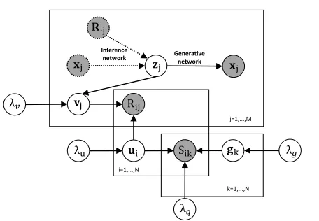
be-ing the highly no-linear function parameterized byθ. According to the graphic model in Fig.1, the joint proba-bility ofR,S,X,U,V,G,Zcan be represented as:

p(O,Z) =YN

i=1

YM

j=1

YN

k=1p(Oijk,Zijk) =

YN

i=1

YM

j=1

YN

k=1p(zj)p(gk)p(ui)pθ(xj|zj)p(vj|zj) p(Rij|ui,vj)p(Sik|ui,gk), (5)

whereO ={R,S,X}is the set of all observed variables, Z ={U,V,G,Z}is the set of all latent variables needed to be inferred, and Oijk = {Rij, Sik,xj} and Zijk =

{ui,vj,gk,zj}for short.

Bayesian Point Estimation

Previous works (Wang, Wang, and Yeung 2015; Wang and Blei 2011) have shown that using an EM-style algorithm en-ables recommendation methods that integrate them to obtain high-quality latent vectors (in our case,UandV). Inspired by these work, in this section, we first derive an EM-style al-gorithm called BDCMF-1 from the view of Bayesian point estimation. The marginal log likelihood can be given by:

logp(O) = log

Z

p(O,Z)dZ ≥

Z

q(Z) logp(O,Z)

q(Z) dZ

=

Z

q(Z) logp(O,Z)−

Z

q(Z) logq(Z)≡ L(q), (6)

where we apply Jensen’s inequality, and q(Z) and F(q)

are variational distribution and the evidence lower bound

λ𝑣

λu

𝐱j 𝐳j 𝐱j

𝐯j Rij

𝐮i Sik 𝐠k j=1,...,M

i=1,...,N

k=1,...,N

λ𝑔

λ𝑞 Generative

network Inference

network

𝑅·𝑗 𝐑·j

Figure 1: Graphical model of our BDCMF. Solid and dashed lines represent generative and inference process, respec-tively. Shaded nodes represent observed variables.

(ELBO), respectively. For variational distributionq(Z), we consider variational distributions in it to be matrix-wise in-dependent:

q(Z) =q(U)q(V)q(G)q(Z) (7)

=YN

i=1q(ui)

YM

j=1q(vj)

YN

k=1q(gk)

YM

j=1q(zj). For Bayesian point estimation, we assume the variational distribution ofuiis:

q(ui) =

YD

d=1δ(Uid−

ˆ

Uid), (8)

where{Uˆid}Dd=1are variational parameters andδis a Dirac delta function. Variational distributions ofvjandgkare

de-fined similarly. WhenUid is discrete (The continuous

situ-ation will be discussed in next section), the entropy ofui

is:

H(ui) =− Z

q(ui) logq(ui) (9)

=XD

d=1

X

Uid

δ(Uid−Uˆid) logδ(Uid−Uˆid) = 0.

Similarly, H(vj)andH(gk)are 0 when the elements are

discrete. Then the evidence lower boundL(q)(Eq. 6) can be written as:

Lpoint( ˆU,Vˆ,Gˆ, θ, φ) =hlogp(U)p(G)p(V|Z) (10) p(X|Z)p(R|U,V)p(S|U,G)iq−KL(qφ(Z|X)||p(Z)),

where h·iis the statistical expectation with respect to the

corresponding variational distribution.Uˆ = nUˆid o

,Vˆ =

n

ˆ

Vjd o

and Gˆ = nGˆkd o

are variational parameters

cor-responding to the variational distribution q(U), q(V)and q(G), respectively.

and Welling 2014), traditional variational-EM algorithm (Neal and Hinton 1998) is intractable to infer the pos-terior of Z. Consequently, similar to VAE (Kingma and Welling 2014), we also introduce a variational distribution qφ(Z|X,R)to approximate the true posterior distribution

p(Z|O).qφ(Z|X,R)is implemented by a inference neural

network parameterized byφ(see Fig.1). Specifically, forzj

we have:

q(zj) =qφ(zj|xj,R·j) =N(µj,diag(δj2)), (11)

where the meanµj and variance δj are the outputs of the

inference neural network.

Directly maximizing the ELBO (Eq. 10) involves solving parametersUˆ,Vˆ Gˆ,θandφ, which is intractable. Thus, we derive an iterative variational-EM (VEM) algorithm to max-imizeLpoint( ˆU,Vˆ,Gˆ, θ, φ), abbreviatedLpoint.

Variational E-step. We first keepθandφfixed, then opti-mize evidence lower boundLpointwith respect toUˆ,Vˆ and

ˆ

G. The updating rules ofuˆi, ˆvj andgˆk are (we omit the

derivation due to space limitations):

ˆ

ui←( ˆVCiVˆ>+λqGEˆ iGˆ>+λuID)−1·

( ˆVCiRi+λqGEˆ iSi), (12)

ˆ

vj←( ˆUCjUˆ>+λvID)−1( ˆUCjRj+λvhzji), (13)

ˆ

gk ←(λqUEˆ kUˆ>+λgID)−1(λqUEˆ kSk), (14)

whereCi=diag(ci1, ...ciM),Ei =diag(ei1, ...eiN),Ri=

[Ri1, ...RiM]andSi = [Si1, ...SiN]. For item latent vector

vj and social latent vectorgk,Cj,Rj,Ek andSk are

de-fined similarly.uˆi = [ ˆUi1, ...UˆiD],vˆj = [ ˆVj1, ...VˆjD]and

ˆ

gk = [ ˆGk1, ...GˆkD]. Forzj, its expectation ishzji = µj,

which is the output of the inference network.

It can be observed thatλv governs how much the latent

item vector zj affects item latent vector vj. For example,

if λv = ∞, it indicates we direct use latent item vector

to represent item latent vectorvj; ifλv = 0, it means we

do not embed any item content information into item latent vector.λq serves as a balance parameter between social

net-work matrix and user-item matrix on user latent vectorui.

For example, ifλq = ∞, it means we only use the social

network information to model user’s preference; ifλq = 0,

we only use user-item matrix and item content information for prediction. Thus,λvandλqare regarded as collaborative

parameters for item content, feedback and social matrices.

Variational M-step. KeepUˆ,Vˆ andGˆ fixed, we optimize the followingLpointw.r.t.φandθ(we only focus on terms containingφandθ):

Lpoint=constant+XM

j=1L(θ, φ;xj,vj,R·j) =constant

+XM

j=1− λv

2 h(vj−zj)

>_(v

j−zj)iq(Z)+ (15) hlogpθ(xj|zj)iqφ(zj|xj,R·j)−KL(qφ(zj|xj,R·j)||p(zj)),

whereM is the number of items and the constant term rep-resents terms which do not containθandφ. For the expec-tation termhpθ(xj|zj)iqφ(zj|xj,R·j), we can not solve it

an-alytically. To handle this problem, we approximate it by the

Monte Carlo sampling as follows:

hlogpθ(xj|zj)iqφ(zj|xj,R·j)=

1

L

XL

l=1pθ(xj|z

l j), (16)

whereL is the size of samplings, and zl_j denotes the l-th sample, which is reparameterized tozl

j =ljdiag(δj2)+µj.

Herel

j is drawn fromN(0,ID)andis an element-wise

multiplication. By using this reparameterization trick and Eq 11,L(θ, φ;xj,vj,R·j)in Eq 15 can be estimated by:

L(θ, φ;xj,vj,R·j)'L˜j(θ, φ) =−

λv

2 (−2µ

>

jvˆj+

µ>_jµj+ tr(diag(δj2))) +

1

L

XL

l=1pθ(xj|z

l j)

−KL(qφ(zj|xj,R·j)||p(zj)) +constant. (17)

We can construct an estimator of Lpoint(φ, θ;X,V,R), based on minibatches:

Lpoint(θ, φ)'L˜P(θ, φ) = M

P

XP

j=1

˜

Lj_{(θ, φ). (18)}

As discussed in (Kingma and Welling 2014), the number of samplingsLper itemj can be set to 1 as long as the mini-batch sizePis large enough, e.g.,P = 100. We can update θandφby using the gradient∇θ,φL˜P(θ, φ).

We iteratively updateU,V,G, θ,andφuntil it converges. Overview of our Bayesian point estimation is summarized in algorithm 1.

Bayesian Posterior Estimation

We assume Uˆ, Vˆ and Gˆ are discrete variables. When these variables are continuous, as discussed in pervi-ous work (Welling, Chemudugunta, and Sutter 2008), the Bayesian point estimation will lead overly to optimistic esti-mates of test-set log-likelihood. This problem is exactly that pervious well-known recommendation models such CTR-based and CDL-CTR-based models (Wang, Wang, and Yeung 2015; Wang and Blei 2011; Purushotham, Liu, and Kuo 2012; Chen et al. 2014; Zhang et al. 2016) which use point estimation algorithm suffer from. In addition, point estima-tors leads to higher variance in prediction and ignore un-certainty in the model parameters. Unlike CTR-based and CDL-based recommendation methods, BDCMF can be eas-ily estimated by a full Bayesian posterior estimator.

Here, we derived Bayesian posterior estimation learning algorithm called BDCMF-2. For Bayesian posterior estima-tion, we also assume variational distributions are matrix-wise independent:

q(Z) =q(U)q(V)q(G)q(Z) (19)

=YN

i=1q(ui)

YM

j=1q(vj)

YN

k=1q(gk)

YM

j=1q(zj), For variational distributionsp(zj), we also introduce a

vari-ational distribution qφ(Z|X) to approximate the true

pos-terior distribution p(Z|O) like Bayesian point estimation. qφ(Z|X)is parameterized byφ, an inference neural network

(see Fig.1). Forzj:

It should be noted we do not assume the specific forms of variational distributions for q(ui), q(vj) and q(gk) in

Bayesian posterior estimation. Our goal is also to maximize the evidence lower boundL(q)(Eq. 6). The algorithm also contains variational E-step and M-step.

Variational E-step. we fixθandφ, then optimize evidence lower bound (6) w.r.tui,vjandgk. Taking the derivative of

lower bound (Eq. 6) w.r.t.q(ui)and setting it to zero, then

we can get:

q(ui)∝exp

hlogp(O,Z)iq(Z\ui) =N(ui,Λ

u i), (21)

where the expectation is taken with respect to the variational distributions over all latent variables excludingui. Thus, the

updating rules ofuiare:

q(U) =YM

i=1N(ui,Λ

u

i),where (22)

Λu_i ←(hViCihVi>+

XM

j=1cijΛ

v

j+λq(hGiEihGi>

+XN

k=1eikΛ

g

k) +λuID)−1, (23)

ui ←Λui(hViCiRi+λqhGiEiSi). (24)

Similarly, the updating rules ofVandGare:

q(V) =YM

j=1N(vj,Λ

v

j),where (25)

Λv_j ←(hUiCjhUi>+

XN

i=1cijΛ

u

i +λvID)−1, (26)

vj←Λvj(hUiCjRj+λvhzji). (27)

q(G) =YN

k=1N(gk,Λ

g

k),where (28)

Λg_k←(λq(hUiEkhUi>+

XN

i=1eikΛ

u i)

+λgID)−1, (29)

gk←Λ g

k(λqhUiEkSk). (30)

Variational M-step. we only focus parametersθandφ. The M-step is as same as Bayesian point estimation. By using the reparameterization trick as we did in Bayesian point es-timation, the objection function w.r.tθandφis:

L(q) =constant+XM

j=1L(θ, φ;xj,vj,R·j) =constant

+XM

j=1− λv

2 h(vj−zj)

>_(v

j−zj)iq(Z)+ (31) hlogpθ(xj|zj)iqφ(zj|xj,R·j)−KL(qφ(zj|xj,R·j)||p(zj)).

We can optimize it as the same as we did in Bayesian point estimation.

Discussion

According to Algorithm 1, the time complexity of updat-inggk isO(N D2+D3), whereN is the number of users

andDis the dimension of latent space. The time complex-ity of updatingvj is O(N D2+D3 +LP2), whereL is

the number of layers in neural network andPis the average dimension of these layers. The time complexity of updat-inguiisO(M D2+N D2+D3), whereM is the number

Algorithm 1BDCMF-1 inference algorithm.

Require: user-item matrix R, item content matrix X, pa-rametersλv,λu,λg, andλq, andP = 100andL= 1.

1: Randomly initialize variational parameters uˆi, vˆj, gˆk

and network parametersθandφ. 2: whilenot convergeddo

3: fori= 1toNdo 4: updateuˆiusing Eq.12.

5: end for

6: forj= 1toMdo 7: updatevˆjusing Eq.13.

8: end for

9: fork= 1toNdo 10: updategˆkusing Eq.14.

11: end for

12: randomly draw P triples, i.e., {(xp,vp,R·p)}Pp=1 from the dataset.

13: ←drawP samples fromN(0,ID), with each for a

triple(xp,vp,R·p).

14: θ, φ←updateθ, φusing the gradient∇θ,φL˜P(θ, φ).

15: end while

of items. Because VCˆ iVˆ> in Eq. 12 can be rewritten as

ˆ

V(Ci−ϕ2I) ˆV>+ϕ2VˆVˆ>, the complexity of updatinggk

decreases fromO(N D2+D3)toO(N0D2+D3), where N0is observed rating numbers with respect to itemjwhich is relatively small in sparse matrix.UCˆ jUˆ> andUEˆ kUˆ>

can be rewritten, similarly. In fact, the latent dimensionsDis also relatively small (<200). Therefore, our BDCMF can be very efficient for large datasets. Additionally, our model is flexible to handle different types of contents in different sce-narios by replacing the architecture of neural networks for inferring items’ latent content representations to the other neural networks such as recurrent neural network.

Prediction

After Algorithm 1 is converged, we predict the missing value RijinRby using the learned latent featuresuiandvj:

R∗_ij =hRiji= (hzji+hkji)>huii=hvji>huii. (32)

For a new item that is not rated by any other users, the offset jis zero, and we can predictRijby:

R∗_ij=hRiji=hzji>huii. (33)

Experiments

Experimental Setup

Research Questions. The research questions guiding the remainder of the paper are: (RQ1) How does our proposed BDCMF-1 compare to state-of-the-art MF methods for CF on sparsity matrix? (RQ2) How do different param-eter settings (e.g., the social paramparam-eter λq and content

parameterλv) affect BDCMF-1? (RQ3) Does the Bayesian

posterior estimation outperform Bayesian point estimation?

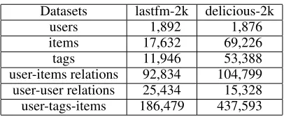
Table 1: Statistics of the datasets.

Datasets lastfm-2k delicious-2k users 01,892 001,876 items 17,632 069,226

tags 11,946 053,388

user-items relations 92,834 104,799 user-user relations 25,434 015,328 user-tags-items 186,479 437,593

Lastfm1(lastfm-2k) and Delicious2(delicious-2k) collected by Brusilovsky et al. (2010). Both of the datasets contain user-item, user-user, and user-tag-item relations. We first transform datasets as implicit feedback. For Lastfm dataset, we consider the user-item feedback is 1 if the user has listened to the artist (item); otherwise, it is 0. Similarly, for the Delicious dataset, if the user has bookmarked a URL (item), the user-item feedback is 1; otherwise, the feedback is 0. After doing so, Lastfm and Delicious datasets only contain 0.27% and 0.08% observed feedbacks, respectively, and are extremely sparse. We use items bag-of-word tag representations as their items content information.

Baselines. For fair comparisons, like that in our BDCMF-1 and BDCMF-2 (in what follows, we use BDCMF to refer to these two models), most baselines we used also incorporate user social information or item content information into matrix factorization.

MF-based methods:

(1) PMF. This model (Mnih and Salakhutdinov 2008) is a famous MF method, and only uses user-item feedback matrix.

(2) SoRec. This model (Ma et al. 2008) jointly decomposes user-user social matrix and user-item feedback matrix to learn user and item latent representations.

Content-based methods:

(3) Collaborative topic regression (CTR). This model (Wang and Blei 2011) utilizes topic model and matrix factorization to learn latent representations of users and items.

(4) Collaborative deep learning (CDL). This model (Wang, Wang, and Yeung 2015) utilizes stack denoising au-toencoder to learn latent items’ content representations, and incorporates them into probabilistic matrix factorization.

Hybrid methods:

(5) CTR-SMF. This model (Purushotham, Liu, and Kuo 2012) incorporates topic modeling and probabilistic MF of social networks.

(6) PoissonMF-CS This model(de Souza da Silva, Langseth, and Ramampiaro 2017), jointly models use social trust, item content and user’s preference using Poisson matrix factorization framework. It is a state-of-the-art MF method for Top-N recommendation on the Lastfm dataset.

Neural network-based method:

(7)Neural Matrix Factorization (NeuMF). This model (He et al. 2017) is a state-of-the-art CF method, which

1

http://www.lastfm.com.

2

http://www.delicious.com.

utilizes neural network to model the interaction between user and item features.

Settings. For fair comparisons, We first set the parameters for PMF, SoRec, CTR, CTR-SMF, CDL, NeuMF via five-fold cross validation. For PMF, we set D,λu andλv

as 50, 0.01 and 0.001, respectively. The parameter settings for SoRec are λc = 10, λu = λv = λz = 0.001. For

CTR, we find it achieve best performance when D=50, λu=0.1, λv=100, a=1 and b=0.01. CTR-SMF yields the

best performance when D=75, λu=0.1, λv=100, λq=100,

a=1 andb=0.01. For CDL, it achieves the best performance when we set a = 1, b = 0.01, D = 50, λu=1, λv=10,

λn = 1000, and λw=0.0001. For NeuMF, we set D=50,

and the last hidden layer is 16. For PoissonMF-CS, we set λc=0.1 and λs=0.1. For our model BDCMF, we set

D=50. We set λv=1, λq=10 for dataset Lastfm, and set

λv=0.1,λq=10 for dataset Delicious. To evaluate our model

performance on extreme sparse matrix, we use 90% of dataset to train our model and the remainder for testing. The dimensions of the layers of the network for BDCMF are (L+N)-200-100(zj)-100-100-(L+N), where L and N are

the dimension ofxj andR·j. The ’-’ denotes the next layer

in neural networks.

Evaluation Metrics. The metrics we used are Re-call@K, NDCG@K and MAP@K which are com-mon metrics for recommendation and their definitions can be found at (Croft, Metzler, and Strohman 2015; Liang and de Rijke 2016). We report the average perfor-mance over all users on the metrics.

Experimental Results and Discussions

Overall Performance (RQ1). Table 2 shows the perfor-mance of our BDCMF-1 and the baselines using the two datasets. According to Table 2, we have following find-ings: a) BDCMF-1 outperforms the baselines in terms of all matrices on Lastfm, which demonstrates the effective-ness of our method of inferring the latent factors of users and items. b) For more sparse dataset, Delicious, BDCMF-1 also achieves the best performance, which demonstrates our model can effectively handle matrix sparsity problem. c) We can see both methods that utilize content and social in-formation (BDCMF-1 and PoissonMF-CS) outperform the others (CDL, CTR, SoRec and PMF), which demonstrates incorporating content and social information can effectively alleviate matrix sparse problem. d) Our BDCMF-1 out-performs state-of-the-art PoissonMF-CS, though they are both Bayesian generative model. The reason is that our BDCMF-1 incorporates neural network into Bayesian gen-erative model, which makes it have powerful non-linearity to model item content’s latent representation.

Impact of Parameters (RQ2).Fig. 2(a) and 2(b) show the contour of Recall@50 by varying content parametersλvand

social parametersλq on Lastfm and Delicious datasets. As

we can see, BDCMF-1 achieves the best recommendation performance whenλv=0.1 and λq=10 in Lastfm. We also

can see that the performance is worse when λv >10, as

λv can control how much item content information is

Table 2: Recommendation performance of BDCMF-1 and the baselines. The best and the second best performance scores per metric per dataset are marked with boldfaces and underlined, respectively.

Lastfm Dataset Delicious Dataset

Recall@20 Recall@50 NDCG@20 MAP@20 Recall@20 Recall@50 NDCG@20 MAP@20 PMF 0.0923 0.1328 0.0703 0.1083 0.0272 0.0561 0.0286 0.0312 SoRec 0.1088 0.1524 0.0721 0.1128 0.0384 0.0892 0.0323 0.0389 CTR 0.1192 0.1624 0.0799 0.1334 0.0563 0.1342 0.0487 0.0581 CTR-SMF 0.1232 0.1832 0.0823 0.1386 0.0781 0.1564 0.0534 0.0588 CDL 0.1346 0.2287 0.0928 0.1553 0.0861 0.1897 0.0726 0.0792 NeuMF 0.1517 0.2584 0.1036 0.1678 0.1078 0.2267 0.0769 0.0928 PoissonMF-CS 0.1482 0.2730 0.1089 0.1621 0.1012 0.2123 0.0742 0.0863 BDCMF-1(ours) 0.1625 0.3026 0.1174 0.1701 0.1121 0.2341 0.0826 0.1021

(a) Lastfm—Recall@50 (b) Delicious—Recall@50

Figure 2: The contour of Recall@50 by varyingλvandλq

on datasets Lastfm and Delicious.

their friends.λq can control how much social information

is incorporated into user latent factor. Thus, our BDCMF-1 is very sensitive to λv and λq. For Delicious dataset,

Fig. 2(b) shows BDCMF-1 achieves the best performance on Recall@50 whenλv =1 andλq =10. Fig. 2(a) and 2(b)

show that we can balance the content information and social information by varyingλv andλq, leading to better

recom-mendation performance.

To figure out the impact of the latent dimensionD, we vary D and see the performance. As shown in Fig. 3, BDCMF-1 outperforms all the baselines with all dimen-sions, which demonstrates BDCMF-1 can learn better latent representations of users and items than the baselines regard-less of their dimensional size.

The Effectiveness of Bayesian posterior estimation (RQ3).To figure out the effectiveness of Bayesian posterior estimation, we make comparison between BDCMF-1 and BDCMF-2 on Lastfm dataset. Results on Delicious show the same trend and thus we omit it here. Performance of BDCMF-1 and BDCMF-2 over iterations on Lastfm is ob-served as: a) With more iterations, the ELBO of BDCMF-1 and BDCMF-2 gradually increases. BDCMF-2 achieves bigger ELBO than 1, which illustrates BDCMF-2 can fit data better (the margin likelihood of data is more higher). b) For recommendation performance, BDCMF-2 outperforms BDCMF-1 in terms of all metrics. Specifi-cally, BDCMF-2 betters with a 10.4% relative improvement on Recall@20. c) When the number of iterations > 30, BDCMF-1 suffers severe overfitting problem (Recall@20 scores begin to decrease, although the EBLO keeps increas-ing). In contrast, BDCMF-2 does not suffer this overfitting

Figure 3: Recommendation performance on Lastfm and De-licious with various values of dimension D.

Figure 4: ELBO and recommendation performance of BD-CMF methods w.r.t. the number of iterations on Lastfm (D=50,λv= 0.1andλq = 10).

Conclusions

In this paper we studied the problem of inferring latent fac-tors of users and items in the social recommender system. We have proposed a novel Bayesian deep collaborative ma-trix factorization model, BDCMF, which incorporates var-ious item content information and user social relationship into a full Bayesian framework. To model item’s latent con-tent vector, we use a generative network to model the gen-erative process of item content. To effectively infer latent factors of users and items, we first derived a EM algorithm from a Bayesian point estimation perspective. Due to the full Bayesian nature of our proposed model and the drawbacks of Bayesian point estimation, we have inferred the full pos-terior distribution of the latent factors of users and items. We have conducted several experiments on two public datasets. Experimental results show that our BDCMF can effective infer latent factors of users and items, and the Bayesian pos-terior estimation is more robust than point estimation. In the future, we will utilize the proposed model to deal with other information retrieval task such as user profiling (Liang 2018; Liang et al. 2018b; Liang, Yilmaz, and Kanoulas 2018) and social network analysis.

References

Adams, R. P.; Dahl, G. E.; and Murray, I. 2014. Incorpo-rating side information in probabilistic matrix factorization with gaussian processes. Papeles De Poblacion3(14):33. Brusilovsky, P.; Koren, Y.; Kuflik, T.; and Weimer, M. 2010. Workshop on information heterogeneity and fusion in rec-ommender systems. InRecSys, 375–376.

Chen, C.; Zheng, X.; Wang, Y.; Hong, F.; and Lin, Z. 2014. Context-aware collaborative topic regression with social ma-trix factorization for recommender systems. InAAAI, 9–15. Croft, W. B.; Metzler, D.; and Strohman, T. 2015. Search engines: Information retrieval in practice. Addison-Wesley Reading.

de Souza da Silva, E.; Langseth, H.; and Ramampiaro, H. 2017. Content-based social recommendation with poisson matrix factorization. InECML-PKDD, 530–546.

Doersch, C. 2016. Tutorial on variational autoencoders.

CoRRabs/1606.05908.

He, X.; Liao, L.; Zhang, H.; Nie, L.; Hu, X.; and Chua, T.-S. 2017. Neural collaborative filtering. InWWW, 173–182. Kingma, D. P., and Welling, M. 2014. Auto-encoding vari-ational bayes. InICLR.

Li, X., and She, J. 2017. Collaborative variational autoen-coder for recommender systems. InKDD, 305–314. Li, S.; Kawale, J.; and Fu, Y. 2015. Deep collaborative filtering via marginalized denoising auto-encoder. InCIKM, 811–820.

Liang, S., and de Rijke, M. 2016. Formal language mod-els for finding groups of experts. Information Processing & Management52(4):529–549.

Liang, S.; Ren, Z.; Weerkamp, W.; Meij, E.; and De Ri-jke, M. 2014. Time-aware rank aggregation for microblog search. InCIKM, 989–998.

Liang, S.; Markov, I.; Ren, Z.; and de Rijke, M. 2018a. Man-ifold learning for rank aggregation. InWWW, 1735–1744. Liang, S.; Zhang, X.; Ren, Z.; and Kanoulas, E. 2018b. Dy-namic embeddings for user profiling in twitter. In KDD, 1764–1773.

Liang, S.; Yilmaz, E.; and Kanoulas, E. 2018. Collabo-ratively tracking interests for user clustering in streams of short texts. IEEE Transactions on Knowledge and Data En-gineering.

Liang, S. 2018. Dynamic user profiling for streams of short texts. InAAAI, 5860–5867.

Lim, Y. J., and Teh, Y. W. 2007. Variational bayesian ap-proach to movie rating prediction. InProceedings of KDD cup and workshop, volume 7, 15–21.

Ma, H.; Yang, H.; Lyu, M. R.; and King, I. 2008. Sorec:social recommendation using probabilistic matrix fac-torization. InCIKM, 931–940.

Mnih, A., and Salakhutdinov, R. R. 2008. Probabilistic ma-trix factorization. InNIPS, 1257–1264.

Neal, R. M., and Hinton, G. E. 1998. A view of the em al-gorithm that justifies incremental, sparse, and other variants. InNato Advanced Study Institute on Learning in Graphical MODELS, 355–368.

Nguyen, T. T., and Lauw, H. W. 2017. Collaborative topic regression with denoising autoencoder for content and com-munity co-representation. InCIKM, 2231–2234.

Park, S.; Kim, Y. D.; and Choi, S. 2013. Hierarchical bayesian matrix factorization with side information. In IJ-CAI, 1593–1599.

Purushotham, S.; Liu, Y.; and Kuo, C. C. J. 2012. Collab-orative topic regression with social matrix factorization for recommendation systems. InICML, 691–698.

Ren, Z.; Liang, S.; Li, P.; Wang, S.; and de Rijke, M. 2017. Social collaborative viewpoint regression with explainable recommendations. InWSDM, 485–494. ACM.

Wang, C., and Blei, D. M. 2011. Collaborative topic model-ing for recommendmodel-ing scientific articles. InKDD, 448–456. Wang, H.; Chen, B.; and Li, W. J. 2013. Collaborative topic regression with social regularization for tag recommenda-tion. InIJCAI, 2719–2725.

Wang, H.; Wang, N.; and Yeung, D. Y. 2015. Collaborative deep learning for recommender systems. In KDD, 1235– 1244.

Welling, M.; Chemudugunta, C.; and Sutter, N. 2008. De-terministic latent variable models and their pitfalls. InSDM, 196–207.

Wu, Y.; DuBois, C.; Zheng, A. X.; and Ester, M. 2016. Col-laborative denoising auto-encoders for top-n recommender systems. InWSDM, 153–162. ACM.

Xu, J.; Yao, Y.; Tong, H.; Tao, X.; and Lu, J. 2017. Hoorays: High-order optimization of rating distance for recommender systems. InKDD, 525–534.