The Thirty-Third AAAI Conference on Artificial Intelligence (AAAI-19)
Universal Approximation Property and Equivalence of Stochastic
Computing-Based Neural Networks and Binary Neural Networks
Yanzhi Wang,
1Zheng Zhan,
2Liang Zhao,
3Jian Tang,
2Siyue Wang,
1Jiayu Li,
2Bo Yuan,
4Wujie Wen,
5Xue Lin
11Department of Electrical and Computer Engineering, Northeastern University, Boston, MA 02115 2Department of Electrical Engineering and Computer Science, Syracuse University, Syracuse, NY 13244
3Department of Mathematics and Computer Science, Lehman College of CUNY, Bronx, NY 10468 4Department of Electrical and Computer Engineering, Rutgers University, Piscataway, NJ 08854 5Department of Electrical and Computer Engineering, Florida International University, Miami, FL 33199
Abstract
Large-scale deep neural networks are both memory and computation-intensive, thereby posing stringent requirements on the computing platforms. Hardware accelerations of deep neural networks have been extensively investigated. Spe-cific forms of binary neural networks (BNNs) and stochastic computing-based neural networks (SCNNs) are particularly appealing to hardware implementations since they can be im-plemented almost entirely with binary operations.
Despite the obvious advantages in hardware implementation, these approximate computing techniques are questioned by researchers in terms of accuracy and universal applicability. Also it is important to understand the relative pros and cons of SCNNs and BNNs in theory and in actual hardware im-plementations. In order to address these concerns, in this pa-per we prove that the ”ideal” SCNNs and BNNs satisfy the universal approximation property with probability 1 (due to the stochastic behavior), which is a new angle from the orig-inal approximation property. The proof is conducted by first proving the property for SCNNs from the strong law of large numbers, and then using SCNNs as a “bridge” to prove for BNNs. Besides the universal approximation property, we also derive an appropriate bound for bit lengthMin order to pro-vide insights for the actual neural network implementations. Based on the universal approximation property, we further prove that SCNNs and BNNs exhibit the same energy com-plexity. In other words, they have the same asymptotic energy consumption with the growth of network size. We also pro-vide a detailed analysis of the pros and cons of SCNNs and BNNs for hardware implementations and conclude that SC-NNs are more suitable.
Introduction
Large-scale neural networks are both memory-intensive and computation-intensive, thereby posing stringent require-ments on the computing platforms when deploying those large-scale neural network models on memory-constrained and energy-constrained embedded devices. In order to over-come these limitations, the hardware accelerations of deep neural networks have been extensively investigated in both industry and academia (Mahajan et al. 2016; Zhao et al.
Copyright c2019, Association for the Advancement of Artificial Intelligence (www.aaai.org). All rights reserved.
2017b; Umuroglu et al. 2017; Han et al. 2016; Chen et al. 2014; Moons et al. 2017). These hardware accelerations are based on FPGA and ASIC devices and can achieve a sig-nificant improvement on energy efficiency, along with small form factor, compared with traditional CPU or GPU based computing of deep neural networks. Both characteristics are critical for the battery-powered embedded and autonomous systems.
Hardware systems, including FPGAs and ASICs, have much higher peak performance for binary operations com-pared to floating point ones. Besides, it is also desirable to reduce the model size of deep neural network such that the whole model can be stored using on-chip memory, thereby reducing the timing and energy overheads of off-chip stor-age and communications. As a result, the Binary Neural Networks (BNNs), proposed by (Courbariaux, Bengio, and David 2015), are particularly appealing since they can be implemented almost entirely with binary operations, with the potential to attain performance in the tera-operations per second (TOPS) range on FPGAs or ASICs.
Besides BNNs, reference work (Ren et al. 2017; Yu et al. 2017; Kyounghoon Kim 2015; Merolla et al. 2014; Li et al. 2018; Neftci 2016; Andreou and Chatzis 2016) have also proposed to utilize the hardware-oriented Stochas-tic Computing (SC) technique for developing (large-scale) deep neural networks, i.e., SCNNs. The SC technique rep-resents a number using the portion of 1’s in a bit sequence. Many key operations in neural networks, such as multiplica-tions and addimultiplica-tions, can be implemented in a single gate in SC. For example, multiplication of two stochastic numbers can be implemented using a single AND gate or XNOR gate (depending on unipolar or bipolar representations). It en-ables the efficient implementation of deep neural networks with extremely small hardware footprint.
Despite the obvious advantages in hardware implemen-tation, these approximate computing techniques are ques-tioned by researchers in terms of accuracy. Will SCNNs and BNNs be accurate for any types of neural networks and ap-plications? More specifically, conventional neural networks with at least one hidden layer satisfy theuniversal approxi-mation property(Cs´aji 2001) in that they can approximate an arbitrary continuous or measurable function given enough number of neurons in the hidden layer. Will SCNNs and BNNs satisfy such property as well? Finally, what are the relative pros and cons of SCNNs and BNNs in theory, and at the hardware level?
In this paper we aim to answer the above questions. We consider the ”ideal” SCNNs and BNNs that are independent of specific hardware implementations. As the key contribu-tion of this paper, we prove that SCNNs and BNNs satisfy the universal approximation property with probability 1 (due to the stochastic behavior in these networks), which is a new angle from the original approximation property. The proof is conducted by first proving the property for SCNNs from the strong law of large numbers, and then using SCNNs as a “bridge” to prove for BNNs. This is because it is difficult to directly prove the property for BNNs, as BNNs represent functions with discrete (binary) input values instead of con-tinuous ones. Besides the universal approximation property, we also derive an appropriate bound for bit lengthM in or-der to provide insights for the actual neural network imple-mentations.
Based on the universal approximation property, we fur-ther prove that SCNNs and BNNs exhibit the same energy complexity. In other words, they have the same asymptotic energy consumption with the growing of network size. We also provide a detailed analysis of the pros and cons of SC-NNs and BSC-NNs for hardware implementations and conclude that SCNNs are more suitable for hardware. It is also possi-ble to strike a desirapossi-ble balance between SCNNs and BNNs to derive the best-suited implementation for a specified hard-ware.
Background and Related Work
Stochastic Computing and SCNNs
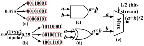
Stochastic computing (SC) is a paradigm that represents a number, named stochastic number, by counting the num-ber of ones in a bit-stream. For example, the bit-stream 0100110100 contains four ones in a ten-bit stream, thus it represents x = P(X = 1) = 4/10 = 0.4. In the bit-stream, each bit is independent and identically distributed (i.i.d.) which can be generated in hardware using stochas-tic number generators (SNGs). Obviously, the length of the bit-streams can significantly affect the calculation accuracy in SC (Brown and Card 2001). In addition to this unipo-lar encoding format, SC can also represent numbers in the range of[−1,1]using the bipolar encoding format. In this scenario, a real number xis processed by P(X = 1) = (x+ 1)/2. Thus 0.4 can be represented by 1011011101, as
P(X = 1) = (0.4 + 1)/2 = 7/10. -0.5 can be represented by 10010000, as it shown in figure 1(b), withP(X = 1) = (−0.5 + 1)/2 = 2/8.
00110001 00101001 10000101 0.375
10110001
10011100 0.25
-0.5(1+x)/2bipolar 00100111
a a×b
b
a
b a×b
M
u
x
1/2 (bit-stream)
a
b
(a+b)/2 (a)
(b)
(c)
(d) (e)
Figure 1: (a) Unipolar encoding format and (b) bipolar en-coding format. (c) AND gate for unipolar multiplication. (d) XNOR gate for bipolar multiplication. (e) MUX gate for ad-dition.
Compared to conventional computing, the major advan-tage of stochastic computing is the significantly lower hard-ware cost for a large category of arithmetic calculations. A summary of the basic computing components in SC, such as multiplication and addition, is shown in Figure 1. As an illustrative example, a unipolar multiplication can be per-formed by a single AND gate since P(A· B = 1) =
P(A= 1)P(B = 1)(assuming independence), and a bipo-lar multiplication is performed by a single XNOR gate since
c = 2P(C = 1)−1 = 2(P(A = 1)P(B = 1) +P(A= 0)P(B= 0))−1 = (2P(A= 1)−1)(2P(B = 1)−1) =
ab.
Besides multiplications and additions, SC-based activa-tion funcactiva-tions are also developed (Li et al. 2017a; 2017b). As a result, SC has become an interesting and promising ap-proach to implement large-scale neural networks (Yuan et al. 2017; Yu et al. 2017; Li et al. 2017c; Kyounghoon Kim 2015) with high performance/energy efficiency and minor accuracy degradation.
We note that the goal of SCNN in approximating using stochastic computation is very different from dropout (or other stochastic techniques). SCNN aims to facilitate hard-ware implementations, and by transforming binary numbers and weights to stochastic ones, it enables efficient imple-mentation with extremely small hardware footprint. This is different from dropout which aims to enhance the generality and robustness.
Binary Neural Networks (BNNs)
BNNs use binary weights, i.e., weights that are constrained to only two possible values (not necessarily 0 and 1) (Cour-bariaux, Bengio, and David 2015). BNNs also have great po-tential to facilitate consumer applications on low-power de-vices and embedded systems. (Zhao et al. 2017b; Umuroglu et al. 2017) have implemented BNNs in FPGAs with high performance and modest power consumption.
The real-valued weights are transformed into the two pos-sible values through the following stochastical binarization operation:
wB=
+1 with probability p=σ(w)
−1 with probability 1−p (1)
whereσis thehard sigmoidfunction:
σ(x) =clip(x+ 1
2 ,0,1) = max(0,min(1,
x+ 1 2 )) (2) A hard sigmoid rather than the soft version is used because it is far less computationally expensive.
At training time, BNNs randomly pick one of two values for each weight, for each minibatch, for both the forward and backward propagation phases of backpropagation. However, the stochastic gradient descent (SGD) update is accumulated in a real-valued variable storing the parameter to average the noise for keeping sufficient resolution. Moreover, binariza-tion process adds some noise into the model, which provides a form of generalization to address the over-fitting problem.
Universal Approximation Property
For feedforward neural networks with one hidden layer, (Cy-benko 1989) and (Hornik, Stinchcombe, and White 1989) have proved separately the universal approximation prop-erty, which guarantees that for any given continuous func-tion or measurable funcfunc-tion and any error bound >0, there always exists a single-hidden layer neural network that ap-proximates the function within integrated error. Besides the approximation property itself, it is also desirable to cast a limit on the maximum amount of neurons. In this direc-tion, (Barron 1993) showed that feedforward networks with one layer of sigmoidal nonlinearities achieve an integrated squared error with order of O(1/n), wherenis the number of neurons.
More recently, several interesting results were published on the approximation capabilities of deep neural networks or neural networks using structured matrices. (Delalleau and Bengio 2011) have shown that there exists certain functions that can be approximated by three-layer neural networks with a polynomial amount of neurons, while two-layer neu-ral networks require exponentially larger amount to achieve the same error. (Montufar et al. 2014) and (Telgarsky 2016) have shown the exponential increase of linear regions as neural networks grow deeper. (Liang and Srikant 2016) proved that with log(1/) layers, the neural network can achieve the error boundfor any continuous function with O(polylog()) parameters in each layer. Recently, (Zhao et al. 2017a) have proved that neural networks represented in structured, low displacement rank matrices preserve the uni-versal approximation property. These recent research have sparked the research interests on the theoretical properties of neural networks with simplifications/approximations which are suitable for high-efficiency hardware implementations.
Neural Network of Interests and SCNNs
Our problem statement follows the flow of reference work (Zhao et al. 2017a) for investigating the universal approxi-mation property. LetIndenote then-dimensional unit cube,
[0,1]n. The space of continuous functions onI
nis denoted
by C(In). A feedforward neural network withN units of
neurons arranged in a single hidden layer is denoted by a functionG:Rn→R, satisfying the form
G(x) = N X
i=1
αiσ(wTix+bi) (3)
wherewi,x ∈ Rn,αi,b
i ∈ R, andσis a nonlinear sig-moidal activation function. Thewi denotes weights associ-ated with hidden neuroniand is applied to inputx.αi de-notes thei-th weight of output neuron, and is applied to the output ofi-th neuron in the hidden layer.biis the bias of unit
i.
Definition 1. A sigmoidal activation functionσ : R → R
satisfies
σ(t)→
1 as t→ ∞
0 as t→ −∞
Definition 2. Starting from the neural network of interests, we define an SCNN satisfying the form:
GSC,M(xSC,M) =
N X
i=1
αiσ(wTSC,M,ixSC,M+bSC,M,i) (4)
where each elementjinwT
SC,M,iis denoted byw j
SC,M,i, and
each element in xSC,Mis denoted byxjSC,M.w
j
SC,M,i,x j
SC,M, and bSC,M,i are stochastic numbers represented by M-bit
streams, as approximations ofwij,xj, andb
i, respectively.
These bit-streams are independent in each bit andwSC,MT ,i, xSC,M, andbSC,M,iwill converge towTi,x, andbi asM → ∞, respectively. The computation inwT
SC,M,ixSC,M+bSC,M,i
follows the SC rules described before.
In the above definitions we focus on an ”ideal” SCNN that assumes accurate activation and output layer calcula-tion (which is reasonable because the output layer size is typically very small). The SCNN of interest, as illustrated in Figure 2, does not depend on specific hardware implementa-tions that may be different in practice. We also do not specify any limitation on the weight and input ranges because they can be effectively dealt with by pre-scaling techniques.
The Universal Approximation Property of
SCNNs and BNNs
In this section, we prove that SCNNs and BNNs satisfy the universal approximation property with probability 1, which is a new angle from the original universal approximation property. More specifically, we first prove the property for SCNNs and then use SCNNs as a ”bridge” to prove for BNNs. This two-step proof is due to the fact that directly proving the property for BNNs is difficult, as BNNs repre-sent functions with binary input values.
(00110010)
(10100010)
(11010010) M bits x1SC,M
x2SC,M
xnSC,M
wSC,M,1
wSC,M,2
wSC,M,N
G
SC
,M
(
x
SC
,M
)
Figure 2: The structure of SCNN of interest.
Universal Approximation Property of SCNN
In this section we will prove a lemma on the closeness of stochastic approximation for the inputs of each neuron, a lemma on the closeness of approximations for the outputs, and finally extend the universal approximation theorem from (Cybenko 1989) to SCNNs.
Lemma 1. As the bit-stream lengthM → ∞, the stochas-tic numberwSCT,M,ixSC,M+bSC,M,iconverges towTix+bi
almost surely.
Proof. LetΩbe the sample space of all bit-streams gener-ated to represent elements inwTi, x, andbi. For each in-stance ω ∈ Ω, use notations wTSC,M,i(ω), xSC,M(ω), and
bSC,M,i(ω)to represent stochastic numbers (or vectors)
cal-culated from the corresponding M-bit streams associated withω. Moreover, define three constant random variables representing the target real values, namely for each i ∈ {1, ..., N},
wT
i(ω)≡wTi,∀ω∈Ω,
x(ω)≡x,∀ω∈Ω, bi(ω)≡bi,∀ω∈Ω,
(5)
We shall prove that for everyω∈Ω:
lim
M→∞w
T
SC,M,i(ω)·xSC,M(ω) +bSC,M,i(ω) =
wTi(ω)·x(ω) +bi(ω).
(6)
From the construction of the random variables, we have that for eachiandj
lim
M→∞w
j
SC,M,i(ω) =w j
i,
lim
M→∞x
j
SC,M(ω) =x
j,
lim
M→∞bSC,M,i(ω) =bi.
Therefore, these exists Mmin(ω) such that for all M ≥
Mmin(ω)and all >0, we have
wjSC,M,i(ω)xSCj ,M(ω)−wjixj <0
bSC,M,i(ω)−bi
<0,
where0= 1
n+1. Use an argument of triangle inequality to show
w
T
SC,M,i(ω)·xSC,M(ω)+bSC,M,i(ω)−wTix−bi
< (7) Sincecan be arbitrarily small, it implies
lim
M→∞w
T
SC,M,i(ω)·xSC,M(ω) +bSC,M,i(ω) =wiTx+bi.
(8) Since this is true for everyω∈Ω, we conclude that
P
ω∈Ω : lim
M→∞w
T
SC,M,i(ω)·xSC,M(ω) +bSC,M,i(ω) =
wiTx+bi = 1.
(9) In other words, we proved that asM → ∞, the stochastic numberwTSC,M,i(ω)·xSC,M(ω) +bSC,M,i(ω)almost surely converges towT
ix+bi.
Lemma 2. If the sigmodial function σ(t) has bounded derivative, then the stochastic number σ(wT
SC,M,ixSC,M +
bSC,M,i)almost surely converge to the real valueσ(wT
ix+
bi)as the bit-stream lengthM → ∞, .
Proof. We have the following inequalities:
σ(wSCT,M,ixSC,M+bSC,M,i)−σ(wiTx+bi)
≤max t
σ0(t)· |wTSC,M,ixSC,M+bSC,M,i−wiTx−bi|
≤ max
t σ0(t)
·
wTSC,M,ixSC,M+bSC,M,i−wiTx−bi
(10)
For the currently utilized activation functions, including sig-moid, tanh (hyperbolic tangent), ReLU functions, there is an upper bound on the derivatives. The maximum abso-lute value of the derivatives is often 1. Then, from the above Lemma 1 about the almost sure convergence of
wT
SC,M,ixSC,M+bSC,M,itowiTx+bi, we arrive at the almost sure convergence ofσ(wT
SC,M,ixSC,M+bSC,M,i).
Based on the above lemmas and the original universal ap-proximation theorem, we arrive at the following universal approximation theorem for SCNNs.
Theorem 1. (Universal Approximation Theorem for SC-NNs). For any continuous functionf(x)defined onIn and
any > 0, we define an event that there exists an SCNN functionGSC,M(xSC,M)in the form of Eqn. (4) that satisfies
lim
M→∞|GSC,M(xSC,M)−f(x)|< . (11)
This event is satisfied almost surely (with probability 1).
Proof. From the universal approximation theorem stated in (Cybenko 1989), we know that there exists a function
G(x)representing a deterministic neural network such that |G(x)−f(x)|< /2for allx∈In. For each positive inte-gerM defineGSC,M(x)as the SCNN function obtained by replacing each parameter ofG(x)with itsM-bit stochastic representation. Then we have
|GSC,M(xSC,M)−f(x)|
=|GSC,M(xSC,M)−G(x) +G(x)−f(x)| ≤ |GSC,M(xSC,M)−G(x)|+|G(x)−f(x)|
Applying Lemma 1 and 2, we can bound the first term as
|GSC,M(xSC,M)−G(x)|=
N X
i=1
αiσ(wTSC,M,ixSC,M+bSC,M,i)−
N X
i=1
αiσ(wTix+bi)
≤ N X
i=1
αi h
σ(wSCT,M,ixSC,M+bSC,M,i)−σ(wiTx+bi)
i
≤ N X
i=1
αi
σ(wSCT,M,ixSC,M+bSC,M,i)−σ(wiTx+bi)
(13)
whereNis the size of the hidden layer in the neural network represented byG(x), andαiis thei-th weight in the output layer.
Deriving from Lemma 2, we know that for 2PN
i=1αi
>
0, with probability 1 there existsMminsuch that
σ(wSCT,M,ixSC,M+bSC,M,i)−σ(wiTx+bi)
<
2PN
i=1αi
(14) for M ≥ Mmin. Incorporating into Eqn. (13) we have |GSC,M(xSC,M)−G(x)| <
2. Further incorporating into Eqn. (12) we have|GSC,M(xSC,M)−f(x)| < forM ≥
Mmin. Thereby we have formally proved that universal
approximation theorem holds with probability 1 for SC-NNs.
Besides the universal approximation property, it is also critical to derive an appropriate bound for bit lengthM in order to provide insights for the actual neural network im-plementations. The next theorem gives an explicit bound on the bit length for close approximation with high probability.
Theorem 2. For the SCNN functionGSC,M in Theorem 1,
letM be any integer that satisfies
M > (n+ 1)
2·N2
2δ . (15)
Then with probability at least 1 − δ,
|GSC,M(xSC,M)−f(x)|< holds for allx∈In.
Proof. Different from the above proof based on the strong law of large numbers (almost sure convergence), deriving bounds is more related to the weak law (convergence in probability). As the former case will naturally ensure the lat-ter, we have the following convergence in probability prop-erty: For any, δ >0, there existsMδ
min, such that for any
M ≥Mδ
min, we have
P rn|GSC,M(xSC,M)−f(x)|< o
>1−δ (16)
Based on a reverse order of the above proof of univer-sal approximation, the above inequality is satisfied when we
have
P rn|GSC,M(xSC,M)−G(x)|<
2 o
>1−δ (17)
Furthermore, the above inequality is satisfied when we have
P r
w
j
SC,M,ix j
SC,M−w j
ixj
<
2(n+ 1)·P
iαi
>1−δ
(18) As each bit in stochastic numberwjSC,M,ix
j
SC,M satisfies a binary distribution with expectationwjixj, the maximum
variance is 1
4. Due to i.i.d. property, the maximum variance (σ2) ofwj
SC,M,ix j
SC,Mis 1
4M. According to the Chebyshev’s
inequalityP r kX−µk ≥kσ
≤ 1
k2, we let 1
k2 =δand obtain
1 2√δM =
2(n+ 1)·P
iαi
(19)
Then we derive an upper bound ofMminδ as
Mminδ ≤
(n+ 1)2· P
iαi
2
2δ ≤
(n+ 1)2·N2
2δ (20)
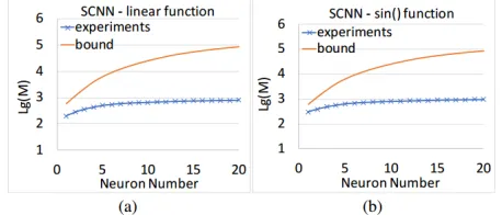
As indicated in the universal approximation theory, any continuous or measurable function in the domain[0,1]ncan be approximated, and this domain matches the input domain of stochastic computing. As a result this bound is a general bound with broad applicability. We conducted multiple ex-periments and all have validated this statement. We demon-strate two experiments shown in (a), (b) in Figure 3. It shows the bound vs. Monte Carlo experiments results, on the bit-sequence lengthM as a function of neuron numberNin the hidden layer. (a) is result on linear function and (b) on sinu-soidal function. The other parameters= 0.2andδ= 0.1.
Figure 3: Illustration of the effect of bound on two types of functions.
Universal Approximation of BNNs and
Equivalence between SCNNs and BNNs
In this section we start from the formal definition of BNNs of interests and then state the universal approximation prop-erty. Similar to the definition of SCNNs, here we focus on an ”ideal” BNN that is independent of actual BNN imple-mentations. An illustration is shown in Figure 4.
x1B
x2B
xmB
wB,1
wB,2
GB(xB)
wB,N
Binary values
Figure 4: The structure of BNN of interest.
Definition 3. A BNN of interest is defined as a function GB(xB), satisfying:
GB(xB) = N X
i=1
αiσ(wTB,ixB+bB,i) (21)
where the input vectorxBand weight vectorwB,ifor eachi
represent vectors of binary values. Letmdenote the dimen-sionality in these two vectors (dimension of inputs).bB,iis a
binary bias value. The computation inwT
B,ixB+bB,ifollows
the BNN rules as described before. Similar to SCNNs, we also consider here accurate activation and output layer cal-culation. This is reasonable and also applied in BNN deploy-ments because the output layer size is typically very small.
The Equivalence of SCNNs and BNNs:The BNNs can be transformed into SCNNs, and vice versa. We illustrate the former case as an example. Let M denote the length of stochastic number and the number of inputs in SCNN
becomes n = m
M. Then the first input stochastic number x1
SC = xB[1 : M](i.e., the firstM bits inxB), the second
input stochastic numberx2
SC = xB[M + 1 : 2M], and so
on. This also applies to the weight stochastic numbers. The bias stochastic numberbSC,ican be a sign extension ofbB,i. In this way the BNN is transformed into SCNN described in Definition 2. The transformation from SCNN to BNN is similar.
Because of the universal approximation property of SC-NNs and the equivalence of BSC-NNs, we arrive at the universal approximation for BNNs as well.
Theorem 3. (Universal Approximation Theorem for BNNs). For any continuous functionf(x)defined onIn, >0, we
define an event that there exists an BNN functionGB(xB)in the form of Eqn. (21) that satisfies
lim
m→∞|GB(xB)−f(x)|< . (22)
This event is satisfied almost surely (with probability 1).
Proof. Apply Theorem 1 to obtain a close approximation of
f(x)with SCNN functions, then build a BNN function that closely approximations the SCNN function.
The equivalence in SCNNs and BNNs also leads to the same bound, defined as the total number of input bitsm=
n·M required to achieve universal approximation. The rea-soning is using proof by contradiction. Suppose that SCNNs have a lower bound, i.e.,n·Mmin < mmin. Then there exists an SCNN with ninputs each with Mmin bits satis-fying the universal approximation property. From the above equivalance analysis we can construct a BNN withMmin·n input bits that also achieves such property, which is smaller and thus in contradiction with the bound mmin. And vice versa.
Energy Complexity and Hardware Design
Implications
Energy Complexity Analysis
The energy complexity, as defined and described in (Mar-tin 2001; Khude, Kumar, and Karnik 2005), specifies the asymptotic energy consumption with the growth of neural network size. It can be perceived as a multiplication of the time complexity and parallelism degree, and therefore is im-portant for hardware implementations and evaluations. As an example, when the input size (number of bits) isn, a rip-ple carry adder has an energy comrip-plexity of O(n) whereas a multiplier has energy complexity of O(n2). On the other hand, both of their time complexity is O(n). The reason is because the ripple carry adder is a sequential computation whereas the multiplier is a parallel computation.
Next we provide an analysis on the energy complexity of the key calculation in wTSC,M,ixSC,M +bSC,M,i in SC-NNs and wT
B,ixB+bB,i in BNNs. From the above equiv-alence analysis, we have m = n·M andM ≥ Mmin for satisfying the universal approximation property. Accord-ing to the hardware implementation details in SCNN and BNN, the multiplication of two bits has energy complex-ity of O(1), then the multiplication of two stochastic num-bers has energy complexity of O(M). The addition of a set of nstochastic numbers has energy complexity of O(nM) using simple calculation units like multiplexers or energy complexity O(nlogn·M) using more accurate accumula-tion units like the approximate parallel counter (APC) (Ky-ounghoon Kim 2015). As a result, the overall energy com-plexity inwT
In fact, one of the key of this work is to show that SCNN and BNN are equivalent, in both functionality and energy complexity. This will shed some light on the neural network implementation because many related work think them not equivalent. As a result this work will draw the attention and provide some guideline about actual implementations.
Hardware Design Implications
Despite the same energy complexity, the actual hardware im-plementations of SCNNs and BNNs are different. As dis-cussed before, SCNNs ”stretch” in the temporal domain whereas BNNs span in the spatial domain. This is in fact the most important advantage of SCNNs. For BNN actual im-plementations, there is often an imbalance between the input I/O size and the computation requirement. The total com-putation requirement (please refer to the energy complexity discussion) is low, but the input requirement is huge even compared with conventional neural networks. This makes actual BNN implementations I/O bound systems, as in ac-tual hardware tapeouts the I/O clock frequency is much lower compared with the computation clock frequency. In other words, the advantage of low and simple computation in BNNs is often not fully exploited in actual deployments (Zhao et al. 2017b; Umuroglu et al. 2017). This limitation can be effectively mitigated by SCNNs, because the spatial requirement is effectively traded-off with the temporal re-quirement. In this aspect SCNNs can use lower I/O account and thereby more effective usage of hardware computation and memory storage resources compared with BNN coun-terparts, thereby becoming more suitable for hardware im-plementations. Of course, the most desirable hardware de-sign is platform-dependent, and will be an effective tradeoff between SCNN and BNN.
On the other hand, BNNs are more heavily optimized in literature compared with SCNNs. Especially, many re-search work (Courbariaux, Bengio, and David 2015; Hubara et al. 2016) are dedicated for effective training methods for BNNs making efficient usage of randomization techniques. On the other hand, the research on SCNNs are mainly from the hardware aspect (Ren et al. 2017; Yu et al. 2017; Li et al. 2017c). For training these work use a straightfor-ward way of transforming directly (every input and weight) from conventional neural networks to stochastic numbers. As a result, it will be effective to take advantage of the train-ing methods for BNNs, transform into SCNNs that are more suitable for hardware implementations using the method de-scribed in the equivalence analysis. In this way, we can ef-fectively exploit the advantage while hiding weakness in both SCNNs and BNNs.
Conclusion
SCNNs and BNNs are low-complexity variants of deep neu-ral networks that are particularly suitable for hardware im-plementations. In this paper, we conduct theoretical analysis and comparison between SCNNs and BNNs in terms of uni-versal approximation property, energy complexity, and suit-ability for hardware implementations. More specifically, we prove that the ”ideal” SCNNs and BNNs satisfy the univer-sal approximation property with probability 1. The proof is
conducted by first proving the property for SCNNs from the strong law of large numbers, and then using SCNNs as a “bridge” to prove for BNNs. Besides the universal ap-proximation property, we also derived an appropriate bound for bit length M in order to provide insights for the ac-tual neural network implementations. Based on the universal approximation property, we further prove that SCNNs and BNNs exhibit the same energy complexity. In other words, they have the same asymptotic energy consumption with the growing of network size. We also provide a detailed analy-sis of the pros and cons of SCNNs and BNNs for hardware implementations and present a way of effectively exploiting the advantage of each type while hiding the weakness.
Acknowledgments
This work is partly supported by the National Science Foun-dation (CNS-1704662, CCF-1733701, and CNS-1739748).
References
Andreou, A. S., and Chatzis, S. P. 2016. Software defect prediction using doubly stochastic poisson processes driven by stochastic belief networks. Journal of Systems and Soft-ware122:72–82.
Barron, A. R. 1993. Universal approximation bounds for superpositions of a sigmoidal function. IEEE Transactions on Information theory39(3):930–945.
Brown, B. D., and Card, H. C. 2001. Stochastic neural computation. i. computational elements.IEEE Transactions on computers50(9):891–905.
Chen, Y.; Luo, T.; Liu, S.; Zhang, S.; He, L.; Wang, J.; Li, L.; Chen, T.; Xu, Z.; Sun, N.; et al. 2014. Dadiannao: A machine-learning supercomputer. InProceedings of the 47th Annual IEEE/ACM International Symposium on Microar-chitecture, 609–622. IEEE Computer Society.
Courbariaux, M.; Bengio, Y.; and David, J.-P. 2015. Bi-naryconnect: Training deep neural networks with binary weights during propagations. InAdvances in neural infor-mation processing systems, 3123–3131.
Cs´aji, B. C. 2001. Approximation with artificial neural net-works.Faculty of Sciences, Etvs Lornd University, Hungary
24:48.
Cybenko, G. 1989. Approximation by superpositions of a sigmoidal function. Mathematics of control, signals and systems2(4):303–314.
David, J. P.; Kalach, K.; and Tittley, N. 2007. Hardware complexity of modular multiplication and exponentiation.
IEEE Transactions on Computers56(10).
Delalleau, O., and Bengio, Y. 2011. Shallow vs. deep sum-product networks. InAdvances in Neural Information Pro-cessing Systems, 666–674.
Hornik, K.; Stinchcombe, M.; and White, H. 1989. Mul-tilayer feedforward networks are universal approximators.
Neural networks2(5):359–366.
Hubara, I.; Courbariaux, M.; Soudry, D.; El-Yaniv, R.; and Bengio, Y. 2016. Quantized neural networks: Training neural networks with low precision weights and activations.
arXiv preprint arXiv:1609.07061.
Khude, N.; Kumar, A.; and Karnik, A. 2005. Time and en-ergy complexity of distributed computation in wireless sen-sor networks. InINFOCOM 2005. 24th Annual Joint Con-ference of the IEEE Computer and Communications Soci-eties. Proceedings IEEE, volume 4, 2625–2637. IEEE.
Kyounghoon Kim, Jongeun Lee, K. C. 2015. Approximate de-randomizer for stochastic circuits. InSoC Design Confer-ence (ISOCC), 2015 International SoC Design ConferConfer-ence. IEEE.
Li, H.; Wei, T.; Ren, A.; Zhu, Q.; and Wang, Y. 2017a. Deep reinforcement learning: Framework, applications, and em-bedded implementations. arXiv preprint arXiv:1710.03792.
Li, J.; Yuan, Z.; Li, Z.; Ding, C.; Ren, A.; Qiu, Q.; Draper, J.; and Wang, Y. 2017b. Hardware-driven nonlinear acti-vation for stochastic computing based deep convolutional neural networks. InNeural Networks (IJCNN), 2017 Inter-national Joint Conference on Neural Networks, 1230–1236. IEEE.
Li, Z.; Ren, A.; Li, J.; Qiu, Q.; Yuan, B.; Draper, J.; and Wang, Y. 2017c. Structural design optimization for deep convolutional neural networks using stochastic computing. InProceedings of the Conference on Design, Automation & Test in Europe, 250–253. European Design and Automation Association.
Li, B.; Najafi, M. H.; Yuan, B.; and Lilja, D. J. 2018. Quan-tized neural networks with new stochastic multipliers. In
2018 19th International Symposium on Quality Electronic Design (ISQED), 376–382. IEEE.
Liang, S., and Srikant, R. 2016. Why deep neu-ral networks for function approximation? arXiv preprint arXiv:1610.04161.
Mahajan, D.; Park, J.; Amaro, E.; Sharma, H.; Yazdan-bakhsh, A.; Kim, J. K.; and Esmaeilzadeh, H. 2016. Tabla: A unified template-based framework for accelerating statis-tical machine learning. InHigh Performance Computer Ar-chitecture (HPCA), 2016 IEEE International Symposium on, 14–26. IEEE.
Martin, A. J. 2001. Towards an energy complexity of com-putation.Information Processing Letters77(2-4):181–187.
Merolla, P. A.; Arthur, J. V.; Alvarez-Icaza, R.; Cassidy, A. S.; Sawada, J.; Akopyan, F.; Jackson, B. L.; Imam, N.; Guo, C.; Nakamura, Y.; et al. 2014. A million spiking-neuron integrated circuit with a scalable communication net-work and interface. Science345(6197):668–673.
Montufar, G. F.; Pascanu, R.; Cho, K.; and Bengio, Y. 2014. On the number of linear regions of deep neural networks. In
Advances in neural information processing systems, 2924– 2932.
Moons, B.; Uytterhoeven, R.; Dehaene, W.; and Verhelst, M. 2017. 14.5 envision: A 0.26-to-10tops/w subword-parallel dynamic-voltage-accuracy-frequency-scalable con-volutional neural network processor in 28nm fdsoi. In
Solid-State Circuits Conference (ISSCC), 2017 IEEE Inter-national, 246–247. IEEE.
Neftci, E. 2016. Stochastic neuromorphic learning machines for weakly labeled data. InComputer Design (ICCD), 2016 IEEE 34th International Conference on, 670–673. IEEE. Ren, A.; Li, Z.; Ding, C.; Qiu, Q.; Wang, Y.; Li, J.; Qian, X.; and Yuan, B. 2017. Sc-dcnn: highly-scalable deep con-volutional neural network using stochastic computing. In
Proceedings of the Twenty-Second International Conference on Architectural Support for Programming Languages and Operating Systems, 405–418. ACM.
Telgarsky, M. 2016. Benefits of depth in neural networks.
arXiv preprint arXiv:1602.04485.
Umuroglu, Y.; Fraser, N. J.; Gambardella, G.; Blott, M.; Leong, P.; Jahre, M.; and Vissers, K. 2017. Finn: A frame-work for fast, scalable binarized neural netframe-work inference. InProceedings of the 2017 ACM/SIGDA International Sym-posium on Field-Programmable Gate Arrays, 65–74. ACM. Yu, J.; Kim, K.; Lee, J.; and Choi, K. 2017. Accurate and efficient stochastic computing hardware for convolu-tional neural networks. InComputer Design (ICCD), 2017 IEEE International Conference on Computer Design, 105– 112. IEEE.
Yuan, Z.; Li, J.; Li, Z.; Ding, C.; Ren, A.; Yuan, B.; Qiu, Q.; Draper, J.; and Wang, Y. 2017. Softmax regression design for stochastic computing based deep convolutional neural networks. InProceedings of the on Great Lakes Sym-posium on VLSI 2017, 467–470. ACM.
Zhao, L.; Liao, S.; Wang, Y.; Tang, J.; and Yuan, B. 2017a. Theoretical properties for neural networks with weight matrices of low displacement rank. arXiv preprint arXiv:1703.00144.