Adaptation Based on Generalized Discrepancy
Corinna Cortes [email protected]
Google Research, 111 8th ave, New York, NY 10011
Mehryar Mohri [email protected]
Andr´es Mu˜noz Medina [email protected]
Courant Institute of Mathematical Sciences, 251 Mercer Street, New York, NY 10012
Editor:Multi Task Learning
Abstract
We present a new algorithm for domain adaptation improving upon a discrepancy minimization algorithm, (DM), previously shown to outperform a number of algorithms for this problem. Unlike many previously proposed solutions for domain adaptation, our algorithm does not consist of a fixed reweighting of the losses over the training sample. Instead, the reweighting depends on the hypothesis sought. The algorithm is derived from a less conservative notion of discrepancy than the DM algorithm called generalized discrepancy. We present a detailed description of our algorithm and show that it can be formulated as a convex optimization problem. We also give a detailed theoretical analysis of its learning guarantees which helps us select its parameters. Finally, we report the results of experiments demonstrating that it improves upon discrepancy minimization.
Keywords: domain adaptation, learning theory
1. Introduction
A standard assumption in statistical learning theory and PAC learning is that training and test samples are drawn from the same distribution (Vapnik, 1998; Valiant, 1984). In practice, however, this assumption often does not hold: the source and target distributions may somewhat differ. This problem is known asdomain adaptationand arises in a variety of applications such as natural language processing and computer vision (Dredze et al., 2007; Blitzer et al., 2007; Jiang and Zhai, 2007; Leggetter and Woodland, 1995; Mart´ınez, 2002; Hoffman et al., 2014). The domain adaptation problem may appear when the distributions over the instance space differ, the so-called covariate shift problem, or when the labeling functions associated with each domain disagree. In practice, a combination of both issues occurs and, for adaptation to succeed, the divergence between the two domains needs to be relatively small. This is clear for the labeling functions since, if the learner receives source labels that are vastly different from the target ones, no learning algorithm can generalize well to the target domain. The same holds when input distributions largely differ.
This intuition was formalized by Ben-David et al. (2010) and Ben-David and Urner (2012) who showed that even in the favorable scenario where the source and target dis-tribution admit the same support, a sample of size in the order of that of the support is needed in order to solve the domain adaptation problem. As the authors point out, the domain adaptation problem becomes intractable when the labeling function for the training
c
data is vastly different from the labeling function used for testing. On the other hand, when some similarity between domains exist, it has been empirically and theoretically shown that adaptation algorithms can be beneficial and in fact a large number of algorithms for this task have been proposed over the past decade. The large majority of them fall in one of the following paradigms:
1. Learning a new feature representation. The core idea behind these algorithms is to map the source and target data into a new feature space where the difference between source and target distributions is reduced. Transfer Component Analysis (TCA) (Pan et al., 2011) and the work on Frustratingly Easy Domain Adaptation (FE) (Daum´e III, 2007) belong to this family of algorithms. Whereas some empirical evidence of the effectiveness of these algorithms exists in the literature, to the best of our knowledge, no work has been done to provide learning guarantees for these algorithms.
2. Reweighting. Originated in the Statistics literature on sample bias correction, these techniques attempt to correct the difference between distributions by multiplying the loss at each training example by a positive weight. Most of the classical algorithms such as KMM (Huang et al., 2006), KLIEP (Sugiyama et al., 2007) and a two-step algorithm by Bickel et al. (2007) fall in this category.
The main focus of this work will be on the latter. A common trait shared by most algorithms in this category is that their reweighting schemes are based on the minimization of a divergence measure between the empirical source and target distributions. For instance, the KL-divergence in the case of KLIEP and the Maximum Mean Discrepancy (MMD) (Gretton et al., 2012) for KMM. The guarantees of these algorithms are therefore given as a function of the chosen divergence. The main drawback of these measures is that they do not take into account the hypothesis set or the loss function, both crucial components of any learning algorithm. In contrast, the discrepancy introduced by Mansour et al. (2009) and further studied by Cortes and Mohri (2011) is a measure of the divergence between distributions tailored to domain adaptation that precisely takes into account both the loss function and the hypothesis set. ThedA-distance, introduced by Devroye et al. (1996)[pp.
271-272] under the name of generalized Kolmogorov-Smirnov distance, later by Ben-David et al. (2006), coincides with the discrepancy when the binary loss function is used. The discrepancy is a pivotal concept used in the analysis of several adaptation scenarios: the Y-discrepancy or integral probability metric (Zhang et al., 2012) was successfully used by Mohri and Mu˜noz (2012) to provide tight learning guarantees for the related task of learning with drifting distributions, whereas a modified version of the discrepancy was used by Germain et al. (2013) to study the problem of domain adaptation in a PAC-Bayesian setting. The discrepancy-based generalization bounds given by Mansour et al. (2009) motivated a discrepancy minimization (DM) algorithm (Cortes and Mohri, 2013), which attempts to minimize said bounds. Besides its favorable theoretical guarantees, this algorithm was shown to perform well in a number of adaptation tasks and to match or outperform several other algorithms such as KMM, KLIEP and the aforementioned two stage algorithm by Bickel et al. (2007).
present an alternative theoretically well founded algorithm for domain adaptation that is based on minimizing a finer quantity, thegeneralized discrepancy, and that seeks to improve upon DM. Unlike the DM algorithm, our algorithm does not consist of afixed reweighting of the losses over the training sample. Instead, the weights assigned to training sample losses vary as a function of the hypothesis h. This helps us ensure that for every hypothesis, h, the empirical loss on the source distribution is as close as possible to the empirical loss on the target distribution for that particular h.
We describe the learning scenario considered (Section 2), then present a detailed descrip-tion of our algorithm and show that it can be formulated as a convex optimizadescrip-tion problem (Section 3). Next, we analyze the theoretical properties of our algorithm, which guide us in choosing the surrogate hypothesis set defining our algorithm (Section 4). In Section 5, we further analyze the optimization problem defining our algorithm and derive an equiva-lent form that can be handled by a standard convex optimization solver. In Section 6, we report the results of experiments demonstrating that our algorithm improves upon the DM algorithm in several tasks.
2. Learning Scenario
This section defines the learning scenario of domain adaptation we consider, which coincides with that of Ben-David et al. (2006) or Mansour et al. (2009); Cortes and Mohri (2013). We first introduce the definitions and concepts needed for the following sections. For the most part, we follow the definitions and notation of Cortes and Mohri (2013).
Let X denote the input space and Y ⊆R the output space. We define a domain as a pair formed by a distribution overX and a target labeling function mapping fromX toY. Throughout the paper, (Q, fQ) denotes the source domain and (P, fP) the target domain withQthe source andP the target distribution overX and withfQ, fP:X → Y the source and target labeling functions, respectively.
In the scenario of domain adaptation we consider, the learner receives two samples: a labeled sample ofmpoints from the source domainS = ((x1, y1), . . . ,(xm, ym))∈(X × Y)m withx1, . . . , xm drawn i.i.d. according toQandyi =fQ(xi) fori∈[1, m]; and an unlabeled
sample T = (x0
1, . . . , x0n)∈ Xn of sizendrawn i.i.d. according to the target distribution P.
We denote by Qb the empirical distribution corresponding to the (unlabeled) sample SX =
(x1, . . . , xm) and byPbthe empirical distribution corresponding toT. We will be in fact more interested in the scenario commonly encountered in practice where, in addition to these two samples, the learner receives a small amount of labeled dataT0 = ((x00
1, y001), . . . ,(x00s, ys00))∈
(X × Y)s from the target domain.
We consider a loss function L: Y × Y →R+ jointly convex in its two arguments. The
Lp losses commonly used in regression and defined by Lp(y, y0) = |y0−y|p for p ≥ 1 are
special instances of this definition. For any two functions h, h0:X → Y and any
distribu-tion D over X, we denote by LD(h, h0) the expected loss of h(x) and h0(x): LD(h, h0) =
Ex∼D[L(h(x), h0(x))]. The learning problem consists of selecting a hypothesis h out of a
hypothesis set H with a small expected loss LP(h, fP) with respect to the target domain.
X Input space Y Output space
P Target distribution Q Source distribution
b
P Empirical target distribution Qb Empirical source distribution
T Target unlabeled sample S Labeled source sample
T0 Small target labeled sample S
X Unlabeled source sample
fP Target labeling function fQ Source labeling function
LP(h,fP) Expected target loss LQ(h,fQ) Expected source loss L
b
P(h,fP) Empirical target loss LQb(h,fQ) Empirical source loss disc(P,Q) Discrepancy DISC(P ,bU) Generalized discrepancy discH00(P,Q) Local Discrepancy discY(P,Q) Y-discrepancy
qmin DM solution Qh GDM solution
Table 1: Notation table.
3. Algorithm
In this section, we describe our new adaptation algorithm. We first review some related previous work. Next, we present the key idea behind our algorithm and derive its general form, and finally, formulate it as a convex optimization problem.
3.1. Previous Work
It was shown by Mansour et al. (2009) and Cortes and Mohri (2011) (see also thedA-distance
(Ben-David et al., 2006) in the case of binary loss for classification) that a key measure of the difference of two distributions in the context of adaptation is the discrepancy. Given a hypothesis set H, the discrepancy, disc, between two distributions P and Q over X is defined by:
disc(P, Q) = max
h,h0∈H
LP(h0, h)− LQ(h0, h)
. (1)
The discrepancy has several advantages over other common divergence measures such as the L1 distance. We refer the reader to (Medina, 2015) for a detailed discussion on this subject. Several generalization bounds for adaptation in terms of the discrepancy have been given in the past (Ben-David et al., 2006; Mansour et al., 2009; Cortes and Mohri, 2011, 2013). including pointwise guarantees in the case of kernel-based regularization algorithms, which includes algorithms such as support vector machines (SVM), kernel ridge regression, or support vector regression (SVR). The bounds given in (Mansour et al., 2009) motivated a discrepancy minimization algorithm. Given a positive semi-definite (PSD) kernel K, the hypothesis returned by the algorithm is the solution of the following optimization problem
min
h∈H λkhk
2
K+Lqmin(h, fQ), (2)
wherek·kKis the norm in the reproducing Hilbert spaceHinduced by the kernelKandqmin is a distribution over the support of Qb such that qmin = argminq∈Qdisc(q,Pb), where Q=
[0,1]SX is the set of all distributions defined over the support of Qb. Besides its theoretical
Observe that, by definition, the objective function optimized by qmin corresponds to a maximum over all pairs of hypotheses. But, the maximizing pair of hypotheses may not be among the candidates ever considered by the learning algorithm. Thus, a learning algorithm based on discrepancy minimization tends to be too conservative.
3.2. Main Idea
From here on we assume the algorithm selected by the learner is an instance of a regu-larized risk minimization algorithm over the Hilbert space H induced by a PSD kernelK. With knowledge of the target labels, these algorithms return a hypothesis h∗ solution of
minh∈HF(h) where
F(h) =λkhk2K+L b
P(h, fP), (3)
whereλ≥0 is a regularization parameter. Thus,h∗ can be viewed as theideal hypothesis. In view of that, we can formulate our objective, in the presence of a domain adaptation problem, as that of finding a hypothesis h whose lossLP(h, fP) with respect to the target
domain is as close as possible to LP(h∗, f
P). To do so, we will seek in fact a hypothesis h
that is as close as possible toh∗, which would imply the closeness of the losses with respect
to the target domains. We do not have access to fP and can only access the labels of the training sampleS. Thus, we must resort to using in our objective function, instead of L
b
P(h, fP), a reweighted empirical loss over the training sampleS. The main idea behind our
algorithm is to define, for any h∈H, a reweighting function Qh:SX ={x1, . . . , xm} →R such that the objective functionG defined for allh∈Hby
G(h) =λkhk2K+LQh(h, fQ) (4)
is uniformly close to F, thereby resulting in close minimizers. Since the first term of (3) and (4) coincide, the idea consists equivalently of seeking Qh such that LQh(h, fQ) and
L b
P(h, fP) be as close as possible. Observe that this departs from the standard reweighting
methods: instead of reweighting the training sample with some fixed set of weights, we allow the weights to vary as a function of the hypothesis h. Note that we have further relaxed the condition commonly adopted by reweighting techniques that the weights must be non-negative and sum to one.
Of course, searching forQhto directly minimize|LQh(h, fQ)−LPb(h, fP)|is in general not possible since we do not have access to fP, but it is instructive to consider the imaginary
case where the average loss L b
P(h, fP) is known to us for any h ∈ H. Qh could then be
determined via
Qh = argmin
q∈F(SX,R)
|Lq(h, fQ)− LPb(h, fP)|, (5)
whereF(SX,R) is the set of real-valued functions defined overSX. For anyh, we can in fact
select Qh such that LQh(h, fQ) =LPb(h, fP) since Lq(h, fQ) is a linear function ofq. Thus, the optimization problem (5) reduces to solving a simple linear equation. With this choice of Qh, the objective functionsF andGcoincide and by minimizingGwe can recover the ideal
solution h∗. Note that, in general, the DM algorithm could not recover that ideal solution.
Even a finer discrepancy minimization algorithm exploiting the knowledge ofL b
P(h, fP) for
in general, recover the ideal solution since we could not have Lq0
min(h, fQ) = LPb(h, fP) for all h∈H.
Of course, L b
P(h, fP) is not accessible since the sampleT is unlabeled. Instead, we will
consider a non-empty convex set of candidate hypotheses H00 ⊆ H that could contain a
good approximation of fP. Using H00 as a set of surrogate labeling functions leads to the following definition ofQh instead of (5):
Qh= argmin
q∈F(SX,R)
max
h00∈H00|Lq(h, fQ)− LPb(h, h
00)|. (6)
The choice of the subset H00 is of course key. Our choice will be based on the theoretical analysis of Section 4. Nevertheless, we now present the formulation of the optimization problem for an arbitrary choice of the convex subsetH00.
Proposition 1 For any h∈H, letQh be defined by (6). Then, the following identity holds
for anyh∈H:
LQh(h, fQ) =
1 2
max
h00∈H00LPb(h, h
00) + min
h00∈H00LPb(h, h
00).
Proof For any h ∈ H, the equation Lq(h, fQ) = l with l ∈ R admits a solution q ∈ F(SX,R). Thus,{Lq(h, fQ) :q∈ F(SX,R)}=Rand for any h∈H, we can write
LQh(h, fQ) = argmin
l∈{Lq(h,fQ) :q∈F(SX,R)}
max
h00∈H00|l− LPb(h, h
00)|
= argmin
l∈R
max
h00∈H00|l− LPb(h, h
00
)| = argmin
l∈R
max
h00∈H00max
n L
b
P(h, h
00)−l, l− L
b
P(h, h
00)o
= argmin
l∈R
maxn max
h00∈H00LPb(h, h
00
)−l, l− min
h00∈H00LPb(h, h
00
)o
= 1 2
max
h00∈H00LPb(h, h
00
) + min
h00∈H00LPb(h, h
00
),
since the minimizing lis obtained for max
h00∈H00LPb(h, h
00)−l=l−min
h00∈H00LPb(h, h
00).
In view of this proposition, with our choice of Qh based on (6), the objective function Gof our algorithm (4) can be equivalently written for allh∈Has follows:
G(h) =λkhk2K+1 2
max
h00∈H00LPb(h, h
00
) + min
h00∈H00LPb(h, h
00
). (7)
Using the fact theL b
P is a jointly convex function, it is easy to show (see for instance Boyd
and Vandenberghe, 2004) that Gis in fact a convex function too.
4. Learning Guarantees
Definition 2 A loss functionLisµ-admissible if there existsµ >0such that the inequality |L(h(x), y)−L(h0(x), y)| ≤µ|h(x)−h0(x)| (8) holds for all(x, y)∈ X × Y andh0, h∈H.
The Lp losses commonly used in regression, p ≥ 1, verify this condition (see Ap-pendix C).
4.1. Rademacher Complexity Bounds
Definition 3 Let Z be any set and G be a family of functions mapping Z to R. Given
a sample S = {z1, . . . , zn} ⊂ Z, the empirical Rademacher complexity of G is denoted by
b
RS(G) and defined by
b
RS(G) =
1
nEσ
sup
g∈G n
X
i=1
σig(zi)
,
where σis, called Rademacher variables, are independent random variables distributed ac-cording to the uniform distribution over{−1,1}. The Rademacher complexity ofGis defined as
Rn(G) = E
S bRS(G)
.
Our first generalization bound is given in terms of the Y-discrepancy, which is a gen-eralization of the discrepancy distance. The Y-discrepancy was first introduced by Mohri and Mu˜noz (2012) in the context of learning with drifting distributions.
Definition 4 The Y-discrepancy between two domains (P, fP) and(Q, fQ) is defined by discY(P, Q) = sup
h∈H
LQ(h, fQ)− LP(h, fP)
.
Note that the definition depends on the labeling functionsfP andfQ. We do not explicitly indicate that dependency for the sake of simplicity of the notation.
We follow the analysis of (Mohri and Mu˜noz, 2012) to derive the following tight gener-alization bounds based on the notion ofY-discrepancy.
Proposition 5 Let HQ and HP be the families of functions defined as follows: HQ := {x 7→ L(h(x), fQ(x)) : h ∈H} and HP := {x 7→ L(h(x), fP(x)) : h ∈H}. Define MQ and MP as MQ = supx∈X,h∈HL(h(x), fQ(x))and MP = supx∈X,h∈HL(h(x), fP(x)). Then, for
anyδ >0,
1. with probability at least 1−δ over the choice of a labeled sample S of size m, the fol-lowing inequality holds for allh∈H:
LP(h, fP)≤ LQb(h, fQ) + discY(P, Q) + 2Rm(HQ) +MQ s
log(1δ)
2m ; (9)
2. with probability at least 1−δ over the choice of a sample T of size n, the following inequality holds for allh∈H and any distribution q over a sampleSX:
LP(h, fP)≤ Lq(h, fQ) + discY(P ,b q) + 2Rn(HP) +MP
s log(1δ)
Proof Let Φ(S) denote suph∈HL b
Q(h, fQ)− LP(h, fP). Changing one point in S changes
Φ(S) by at most MQ
m . Thus, by McDiarmid’s inequality, we haveP Φ(S)−E[Φ(S)]>
≤
e
−2m2 MQ2
. Therefore, for anyδ >0, with probability at least 1−δ, the following holds for all
h∈H:
LP(h, fP)≤ LQb(h, fQ) + E[Φ(S)] +MQ s
log(1δ) 2m .
Next, we can bound E[Φ(S)] as follows: E[Φ(S)] = E
sup
h∈H
L b
Q(h, fQ)− LP(h, fP)
≤E
sup
h∈H
L b
Q(h, fQ)− LQ(h, fQ)
+ sup
h∈H
LQ(h, fQ)− LP(h, fP)
≤2Rm(HQ) + discY(P, Q),
where the last inequality follows from a standard symmetrization inequality in terms of the Rademacher complexity and the definition of discY(P, Q).
For the second bound we have, starting with a standard Rademacher complexity bound forHP, for anyδ >0, with probability at least 1−δ, the following holds for allh∈H:
LP(h, fP)≤ LPb(h, fP) + 2Rn(HP) +MP
s log(1δ)
2n
≤ Lq(h, fQ) +LPb(h, fP)− Lq(h, fQ) + 2Rn(HP) +MP s
log(1δ)
2n . (11)
Moreover, by definitionL b
P(h, fP)−Lq(h, fQ)≤discY(P ,b q) for anyq. Replacing this bound
in (11) yields the result.
Observe that these bounds are tight as a function of the divergence measure (discrep-ancy) we use: in the absence of adaptation, the following standard Rademacher complexity learning bound holds:
L b
P(h, fP)≤ LPb(h, fP) + 2Rn(HP) +MP s
log(1
δ)
2n .
Our second adaptation bound differs from this inequality only by the fact thatL b
P(h, fP) is
replaced withLq(h, fQ) + discY(P ,b q). But, by definition of Y-discrepancy, there exists an
h ∈H such that |L b
P(h, fP)− Lq(h, fQ)|= discY(P ,b q). A similar analysis shows that our
first bound is also tight.
Given a labeled sample S from the source domain, Proposition 5 suggests choosing a distribution q with support SX that minimizes the right-hand side of (10). However, the
quantity discY(P ,b q) depends, by definition, on the unknown labels from the target domain
Let A(H) denote the set of all functions U:h7→Uh mappingH toF(SX,R) such that for allh∈H,h7→ LUh(h, fQ) is a convex function. Thus, for anyh∈H,Uh is a reweighting
function defined over SX. A(H) contains all constant functions U such that Uh =q for all h ∈ H, where q is a distribution over SX. We will abuse the notation and denote this
functions also byq. By Proposition 1,A(H) also includes the function Q:h→Qh used by
our algorithm.
Definition 6 (Generalized discrepancy) For any U ∈ A(H), the generalized discrep-ancy between Pb and U is denoted by DISC(P ,b U) and is defined by
DISC(P ,b U) = sup
h∈H,h00∈H00
|L b
P(h, h
00)− L
Uh(h, fQ)|. (12)
We also denote byd1(fP, H00) theL1 distance offP toH00: d1(fP, H00) = min
h0∈H00
E b
P
|h0(x)−fP(x)|. (13) The following theorem gives an upper bound on theY-discrepancy in terms of the general-ized discrepancy andd1(fP, H00).
Proposition 7 For any distribution q over SX and any set H00, the following inequality
holds:
discY(P ,b q)≤DISC(P ,b q) +µ d1(fP, H00).
Proof Let h0 ∈H00, by the triangle inequality, we can write discY(P ,b q) = sup
h∈H
|Lq(h, fQ)− LPb(h, fP)| ≤ sup
h∈H
|Lq(h, fQ)− LPb(h, h0)|+ sup
h∈H
|L b
P(h, h0)− LPb(h, fP)| ≤ sup
h∈H
max
h00∈H00|Lq(h, fQ)− LPb(h, h
00
)|+ sup
h∈H
|L b
P(h, h0)− LPb(h, fP)|. The hypothesis h0 will later be chosen to minimize the distance of fP to H00. By the
µ-admissibility of the loss, the last term can be bounded as follows: sup
h∈H
|L b
P(h, h0)− LPb(h, fP)| ≤µE b
P
|fP(x)−h0(x)|.
Using this inequality and minimizing overh0∈H00 yields: discY(P ,b q)≤ sup
h∈H
max
h00∈H00|Lq(h, fQ)− LPb(h, h
00)|+µ d1(fP, H00)
= DISC(P ,b q) +µ d1(fP, H00),
which completes the proof.
We can also bound the Y-discrepancy in terms of the discrepancy measure and the following measure of the difference of the source and target labeling functions:
ηH(fP, fQ) = min h0∈H
max
x∈supp(Pb)
|fP(x)−h0(x)|+ max
x∈supp(Qb)
|fQ(x)−h0(x)|
Proposition 8 The following inequality holds for all distributions q over SX:
discY(P ,b q)≤disc(P ,b q) +µ ηH(fP, fQ).
Proof By the triangle inequality and theµ-admissibility of the loss, the following inequality holds for all h0 ∈H:
discY(P ,b q)
= sup
h∈H
|Lq(h, fQ)− LPb(h, fP)|
≤sup
h∈H
|L
b
P(h, h0)− LPb(h, fP)|+|Lq(h, fQ)− Lq(h, h0)|
+ sup
h∈H
|Lq(h, h0)− LPb(h, h0)| ≤µ sup
x∈supp(Pb)
|h0(x)−fP(x)|] + sup
x∈supp(Qb)
[|fQ(x)−h0(x)|]
+ disc(P ,b q).
Minimizing over allh0 ∈H gives discY(P ,b q)≤µ ηH(fP, fQ) + disc(P ,b q) and completes the
proof.
The following learning guarantees are immediate consequences of Propositions 5, 7 and 8.
Corollary 9 Let H00 ⊂ H be a convex set and q a distribution over SX. Then, for any
δ >0, each of the following inequalities holds with probability at least 1−δ for allh∈H:
LP(h, fP)≤ Lq(h, fQ) + DISC(P ,b q) +µ d1(fP, H00) + 2Rn(HP) +MP
s log(1δ)
2n , (14)
LP(h, fP)≤ Lq(h, fQ) + disc(P ,b q) +µ ηH(fP, fQ) + 2Rn(HP) +MP
s log(1
δ)
2n . (15)
In general, the bounds (14) and (15) are not comparable. However, when L is an LP
loss for somep≥1, we can show the existence of a setH00 for which (14) is a tighter bound
than (15). The result is expressed in terms of the local discrepancy defined by: discH00(P ,b q) = sup
h∈H,h00∈H00
|L b
P(h, h
00)− L
q(h, h00)|,
which is a finer measure than the standard discrepancy for which the supremum is defined over a pair of hypothesesboth inH⊇H00.
Theorem 10 Let L be the LP loss for somep≥1. Let H:={B(r) :r≥0} be a set of all
balls B(r) ={h00∈H|L
q(h00, fQ) ≤rp}. Then, for any distribution q over SX, there exists
H00∈H such that the following holds:
Proof Fix a distribution q overSX. Let h∗0 be an element of argminh0∈H LPb(h0, fP)
1
p +
Lq(h0, fQ)
1
p. Choose H00 ∈H as H00 ={h00 ∈ H|L
q(h00, fQ) ≤ rp} with r =Lq(h∗0, fQ)
1
p.
Then, by definition,h∗0is inH00. For theLploss, it is not hard to show that for allh, h00∈H, |Lq(h, h00)− Lq(h, fQ)| ≤ µ[Lq(h00, fQ)]
1
p (see Appendix C). In view of this inequality, we
can write:
DISC(P ,b q) = sup
h∈H,h00∈H00
|L b
P(h, h
00)− L
q(h, fQ)|
≤ sup
h∈H,h00∈H00
|L b
P(h, h
00
)− Lq(h, h00)|+ sup
h∈H,h00∈H00
|Lq(h, h00)− Lq(h, fQ)|
≤discH00(P ,b q) + max
h00∈H00µ[Lq(h
00
, fQ)]1p
= discH00(P ,b q) +µr= discH00(P ,b q) +µLq(h∗0, fQ)
1
p.
Using this inequality, Jensen’s inequality, and the fact that h∗0 is inH00, we can write
µ d1(fP, H00) + DISC(P ,b q)
≤µ min
h0∈H00
E
x∈Pb
[|fP(x)−h0(x)|] +µLq(h∗0, fQ)
1
p + disc
H00(P ,b q)
≤µ min
h0∈H00
E
x∈Pb
[|fP(x)−h0(x)|p]
1
p +µLq(h∗
0, fQ)
1
p + disc
H00(P ,b q)
≤µL b
P(h
∗
0, fP)
1
p +µL
q(h∗0, fQ)
1
p + disc
H00(P ,b q).
Moreover, by definition of h∗0 the last expression is equal to
µ min
h0∈H
L
b
P(h0, fP)
1
p +L
q(h0, fQ)
1
p
+ discH00(P ,b q)
≤µ min
h0∈H
max
x∈supp(Pb)
|fP(x)−h0(x)|+ max
x∈supp(Qb)
|fQ(x)−h0(x)|+ discH00(P ,b q)
=µ ηH(fP, fQ) + discH00(P ,b q).
which concludes the proof.
Theorem 10 shows that the generalized discrepancy can provide a finer measure of the difference between two domains for some choices ofH00. Therefore, for a good choice ofH00, an algorithm minimizing the right-hand side of (14) would benefit from better theoretical guarantees than the DM algorithm. However, the optimization problem defined by (14) is not jointly convex in q and h. Instead, we propose to first minimize the generalized discrepancy and then use this reweighting function as input to our learning algorithm. Further motivation for this two-stage algorithm is given in the following section.
4.2. Pointwise Guarantees
Theorem 11 (Cortes and Mohri, 2013) Let qbe an arbitrary distribution overSX and
let h∗ and hq be the hypotheses minimizing λkhk2K +LPb(h, fP) and λkhk2K +Lq(h, fQ)
respectively. Then, the following inequality holds:
λkh∗−hqk2K ≤µ ηH(fP, fQ) + disc(P ,b q). (16)
Notice that the solution of DM minimizes the right-hand side of (16), that is disc(P ,b q). The following theorem provides an analogous bound for our algorithm.
Theorem 12 Let U be an arbitrary element of A(H) and let h∗ and hU be the hypotheses
minimizing λkhk2
K +LPb(h, fP) and λkhk 2
K +LUh(h, fQ) respectively. Then, the following
inequality holds for any convex set H00⊆H:
λkh∗−hUk2K ≤µ d1(fP, H
00
) + DISC(P ,b U). (17) Proof Fix U ∈ A(H) and let G
b
P denote h 7→ LPb(h, fP) and GU the function h 7→ LUh(h, fQ). Since h 7→ λkhk2K +GPb(h) is convex and differentiable and since h
∗ is its
minimizer, the gradient is zero at h∗, that is 2λh∗ = −∇GPb(h∗). Similarly, since h 7→
λkhk2
K+GU(h) is convex, it admits a sub-differential at anyh∈H. SincehUis a minimizer,
its sub-differential at hU must contain 0. Thus, there exists a sub-gradientg0 ∈∂GU(hU)
such that 2λhU = −g0, where ∂GU(hU) denotes the sub-differential of GU at hU. Using
these two equalities we can write 2λkh∗−hUk2K =hh
∗−
hU, g0− ∇GPb(h∗)i=hg0, h∗−hUi − h∇GPb(h∗), h∗−hUi
≤GU(h∗)−GU(hU) +GPb(hU)−GPb(h
∗
) =L
b
P(hU, fP)− LUh(hU, fQ) +LUh(h
∗, f
Q)− LPb(h
∗, f
P)
≤2 sup
h∈H
|L b
P(h, fP)− LUh(h, fQ)|,
where we used for the first inequality the convexity ofGU combined with the sub-gradient
property of g0 ∈ ∂GU(hU), and the convexity of GPb. For any h ∈ H, using the µ -admissibility of the loss, we can upper bound the operand of the max operator as follows:
|L b
P(h, fP)− LUh(h, fQ)| ≤ |LPb(h, fP)− LPb(h, h0)|+|LPb(h, h0)− LUh(h, fQ)| ≤µ E
x∼Pb
|fP(x)−h0(x)|+ max
h00∈H00|LPb(h, h
00
)− LUh(h, fQ)|,
where h0 is an arbitrary element of H00. Since this bound holds for allh0 ∈H00, it follows immediately that
λkh∗−hUk2K ≤µ min h0∈H00
E b
P
|fP(x)−h0(x)|+ sup
h∈H
max
h00∈H00|LPb(h, h
00)− L
Uh(h, fQ)|,
which concludes the proof.
Note that our choice of Q: h 7→ Qh minimizes the right-hand side of (17) among all
functions U∈ A(H) since, for any U, we can write DISC(P ,b U) = sup
h∈H
max
h00∈H00|LPb(h, h
00
)−LUh(h, fQ)| ≥sup
h∈H
min
q∈F(SX)
max
h00∈H00|LPb(h, h
00
)−Lq(h, fQ)|
= sup
h∈H
max
h00∈H00|LPb(h, h
00)− L
Thus, in view of Theorem 10, for any constant function U ∈ A(H) with Uh =q for some
fixed distribution q over SX, the right-hand side of the bound of Theorem 11 is lower
bounded by the right-hand side of the bound of Theorem 12, since the local discrepancy is a finer quantity than the discrepancy: discH00(P ,b q) ≤disc(P ,b q). Thus, as expected from
the discussion after Theorem 10, our algorithm benefits from a more favorable guarantee than the DM algorithm for some particular choices of H00, especially since, our choice of Q is based on the minimization over all elements inA(H) and not just the subset of constant functions mapping to a distribution. The following pointwise guarantee follows directly from Theorem 12.
Corollary 13 Leth∗ be a minimizer ofλkhk2
K+LPb(h, fP)andhQa minimizer ofλkhk 2
K+
LQh(h, fQ). Then, the following holds for any convex setH00⊆H and for all(x, y)∈ X ×Y:
|L(hQ(x), y)−L(h∗(x), y)| ≤µR
s
µ d1(fP, H00) + DISC(P ,b Q)
λ , (18)
where R2= sup
x∈XK(x, x).
Proof By the µ-admissibility of the loss, the reproducing property of H, and the Cauchy-Schwarz inequality, the following holds for allx∈ X and y∈ Y:
|L(hQ(x), y)−L(h∗(x), y)| ≤µ|hQ(x)−h∗(x)|
=µ|hhQ−h∗, K(x,·)iK|
≤µkhQ−h∗kK
p
K(x, x)≤RkhQ−h∗kK.
Upper bounding khQ −h∗kK using Theorem 12 and using the fact that Q:h → Qh is a
minimizer of the bound over all choices ofU∈ A(H) yields the desired result.
The pointwise loss guarantee just presented can be directly used to bound the difference of the expected loss of h∗ and h
Q in terms of the same upper bounds, e.g.,
LP(hQ, fP)≤ LP(h∗, fP) +µR
s
µ d1(fP, H00) + DISC(P ,b Q)
λ . (19)
Similarly, Theorem 10 directly implies the following Corollary. Corollary 14 Leth∗ be a minimizer ofλkhk2
K+LPb(h, fP)andhQa minimizer ofλkhk 2
K+
LQh(h, fQ). Letsupx∈XK(x, x) =R
2. Then, there exists a choice of H00∈H for which the
following inequality holds uniformly over over (x, y)∈ X × Y:
|L(hQ(x), y)−L(h∗(x), y)| ≤µR
s
µηH(fP, fQ)+discH00(P ,b qmin)
λ ,
The choice of the setH00defining our algorithm is strongly motivated by the theoretical
results of this section. In view of Theorem 10, we restrict our choice ofH00to the familyH, parametrized only by the radiusr. Since the generalized discrepancy DISC is a function of the set H00 which in turn depends only on r, the radiusr is chosen to minimize (19). This
can be done by using as a validation set a small amount of labeled data from the target domain which is typically available in practice. In particular, as the size of the unlabeled sample T0 increases, our estimate of the optimal radius r becomes more accurate. We
provide a detailed description of our algorithm’s implementation in Section 5. 4.3. Comparison against Other Learning Bounds
We now compare the learning bounds just derived for our algorithm with those of some common reweighting techniques. In particular, we compare our bounds with those of Cortes et al. (2008) for the KMM algorithm. A similar comparison however can be derived for other algorithms based on importance weighting such as KLIEP or uLSIF.
Assume P and Q admit densities p and q respectively. For every x∈ X we denote by
β(x) = qp((xx)) the importance ratio and by β =βS
X its restriction to SX. We also let βbbe
the solution to the optimization problem solved by the KMM algorithm. Lethβ denote the solution to
min
h∈H
λkhk2+Lβ(h, fQ), (20)
and h
b
β be the solution to
min
h∈H
λkhk2+L b
β(h, fQ). (21)
The following proposition due to Cortes et al. (2008) relates the error of these hypotheses. The proposition requires the kernelK to be a strictly positive definite universal kernel, with Gram matrix Kgiven byKij =K(xi, xj).
Proposition 15 AssumeL(h(x), y)≤1 for all(x, y)∈ X × Y, h∈H. For anyδ >0, with probability at least 1−δ we have:
|LP(hβ, fP)− LP(hβb, fP)| ≤
µ2R2λmax(K)12
λ
B0
√
m
+ κ 1/2
λ1min/2(K) r
B02
m +
1
n
1 +
r 2 log2
δ
, (22)
whereandB0 are the hyperparameters defining the KMM algorithm andλmax(K), λmin(K) denote the largest and smallest eigenvalues of K respectively.
This bound and the one obtained in (19) are of course not comparable since the depen-dence on µ, R and λ is different. In some cases this dependency can be more favorable in (22) whereas for other values of these parameters (19) provides a better bound. Moreover, (22) depends on the condition number of K which can become really large in practice. However, the most important difference between these bounds is that (19) is given in terms of the ideal hypothesish∗ while (22) is given in terms ofh
β, which, in view of the results of
4.4. Scenario of Additional Labeled Data
Here, we consider a rather common scenario in practice where, in addition to the labeled sample S drawn from the source domain and the unlabeled sample T from the target domain, the learner receives a small amount of labeled data from the target domain T0 =
((x001, y100), . . . ,(x00s, y00s))∈(X × Y)s. This sample is typically too small to be used solely to
train an algorithm and achieve a good performance. However, it can be useful in at least two ways that we discuss here.
One important benefit of T0 is to serve as a validation set to determine the parameter
r that defines the convex set H00 used by our algorithm. The sample T0 can also be used
to enhance the discrepancy minimization algorithm as we now show. Let Pb0 denote the empirical distribution associated with T0. To take advantage ofT0, the DM algorithm can be trained on the sample of size (m+s) obtained by combiningSandT0, which corresponds
to the new empirical distribution Qb0 = m m+sQb+
s m+sPb
0. Note that for a fixed value m and
large values of s, Qb0 essentially ignores the points from the source distribution Q, which corresponds to the standard supervised learning scenario in the absence of adaptation. Let q0min denote the discrepancy minimization solution when using Qb0. Since supp(Qb0) ⊇
supp(Qb), the discrepancy usingq0min is a lower bound on the discrepancy using qmin: disc(q0min,Pb) = min
supp(q)⊆supp(Qb0)
disc(P ,b q)≤ min supp(q)⊆supp(Qb)
disc(P ,b q) = disc(qmin,Pb).
5. Optimization Solution
As shown in Section 3.2, the function G defining our algorithm is convex and the prob-lem of minimizing the expression (7) is a convex optimization probprob-lem. Nevertheless, the problem is not straightforward to solve, in particular because evaluating a term like maxh00∈H00L
b
P(h, h
00) that it contains requires solving a non-convex optimization problem.
Here, we present an exact solution in the case of the L2 loss by solving a semi-definite programming (SDP) problem.
5.1. SDP Formulation
As discussed in Section 4, the choice of H00 is a key component of our algorithm. In view of Corollary 14, we will consider the set H00={h00| Lqmin(h
00, fQ)≤r2}. Equivalently, as a result of the reproducing property ofHand the representer theorem,H00 may be defined as {a∈Rm|Pm
j=1qmin(xj)(Pmi=1aiqmin(xi)1/2K(xi, xj)−yj)2 ≤r2}. Also by the representer
theorem, the solution to (7) will be of the form h = n−1/2Pn
i=1biK(x
0
i,·). Therefore,
given normalized kernel matricesKt, Ks,Kst defined respectively as Ktij =n−1K(x0i, x0j),
Kijs =qmin(xi)1/2qmin(xj)1/2K(xi, xj) andKijst=n−1/2qmin(xj)1/2K(x0i, xj), problem (7) is
equivalent to
min
b∈Rn
λb>Ktb+
1 2
max
a∈Rm kKsa−yk2≤r2
kKsta−Ktbk2+ min a∈Rm kKsa−yk2≤r2
kKsta−Ktbk2
, (23)
wherey= (qmin(x1)1/2y
h0 g1(h) = 0
g2(h) = 0
h0+ ⇤bh
Friday, February 7, 2014
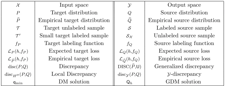
Figure 1: Illustration of the sampling process on the set H00.
Lemma 16 The Lagrangian dual of the problem
max
a∈Rm kKsa−yk2≤r2
1
2kKstak 2−b>
KtKsta,
is given by
min
η≥0,γ γ
s.t. − 1 2K
>
stKst+ηK2s 12K
>
stKtb−ηKsy
1 2b
>K
tKst−ηy>Ks η(kyk2−r2) +γ
! 0.
Furthermore, the duality gap for these problems is zero.
The proof of the lemma is given in Appendix A. The lemma helps us derive the following equivalent SDP formulation for our original optimization problem. Its solution can be found in polynomial time using standard convex optimization solvers.
Proposition 17 The optimization problem (23) is equivalent to the following SDP: max
α,β,ν,Z,z
1 2Tr(K
>
stKstZ)−β−α
s. t νK 2
s+12K
>
stKst−14Ke νKsy+14Kze νy>Ks+14z>Ke α+ν(kyk2−r2)
!
0 λKt+K 2
t 12KtKstz 1
2z
>K>
stKt β
! 0
Z z
z> 1
0∧ν ≥0∧Tr(K2sZ)−2y>Ksz+kyk2≤r2,
where Ke =K>stKt(λKt+K2t)†KtKst, and A† denotes the pseudo-inverse of matrix A.
In the following section we derive a more efficient approximate solution to the optimization problem using sampling, which helps reducing the problem to a simple QP.
5.2. QP Formulation
minimum enclosing ball (MEB) problem. For a set D⊆Rd, the MEB problem is defined
as follows:
min
u∈Rd
max
v∈D ku−vk
2.
Omitting the regularization and the min term from (7) leads to a problem similar to the MEB. Thus, we could benefit from the extensive literature and algorithmic study available for this problem (Kumar et al., 2003; Sch˝onherr, 2002; Yildirim, 2008). However, to the best of our knowledge, there is currently no solution available to this problem in the case of an infinite set D, as in the case of our problem. Instead, we present a solution for solving an approximation of (7) based on sampling.
Let {h1, . . . , hk} be a set of hypotheses on the boundary of H00, ∂H00 and let C = C(h1, . . . , hk) denote their convex hull. The following is the sampling-based approximation
of (7) that we consider:
min
h∈H
λkhk2
K+
1
2i=1max,...,kLPb(h, hi) + 1
2minh0∈CLPb(h, h
0). (24)
Proposition 18 Let Y = (Yij) ∈ Rn×k be the matrix defined by Yij = n−1/2hj(x0i) and
y0 = (y0
1, . . . , y0k)> ∈ Rk the vector defined by y0i = n−1
Pn
j=1hi(x0j)2. Then, the dual
problem of (24) is given by max
α,γ,β −
Yα+γ 2
>
Kt
λI+ 1 2Kt
−1
Yα+γ 2
−1
2γ
>K
tK†tγ+α
>y0−β (25)
s.t. 1>α= 1
2, 1β≥ −Y
>
γ, α≥0,
where 1 is the vector in Rk with all components equal to 1. Furthermore, the solution h
of (24) can be recovered from a solution (α,γ, β) of (25) by ∀x, h(x) = Pni=1aiK(xi, x), where a= λI+1
2Kt)
−1(Yα+1 2γ).
The proof of the proposition is given in Appendix B. The result shows that, given a finite sampleh1, . . . , hkon the boundary ofH00, (24) is in fact equivalent to a standard QP.
Hence, a solution can be found efficiently with one of the many off-the-shelf algorithms for quadratic programming.
We now describe the process of sampling from the boundary of the set H00, which is
a necessary step for defining problem (24). We consider compact sets of the form H00 := {h00∈H|gi(h00)≤0}, where the functions gi are continuous and convex. For instance, we could consider the set H00 defined in the previous section. More generally, we can consider
a family of setsH00
p ={h00∈H| |
Pm
i=1qmin(xi)|h(xi)−yi|p ≤rp}.
Assume that there existsh0 satisfyinggi(h0)<0. Our sampling process is illustrated by Figure 1 and works as follows: pick a random directionbh and defineλi to be the minimal
solution to the system
(λ≥0)∧(gi(h0+λbh) = 0).
Setλi =∞ if no solution is found and defineλ∗= miniλi. By the convexity and
assume that gi(h0+λ∗bh)>0 for somei. The continuity of gi would imply the existence of λ0i with 0< λ0i < λ∗ ≤λi such that gi(h0+λ0ibh) = 0. This would contradict the choice of λi, thus, the inequalitygi(h0+λ∗bh)≤0 must hold for all i.
Since a point h0 with gi(h0) < 0 can be obtained by solving a convex program and solving the equations defining λi is, in general, simple, the process described provides an
efficient way of sampling points from the convex set H00.
5.3. Implementation for the L2 Loss
We now describe how to fully implement our sampling-based algorithm for the case where
L is equal to the L2 loss. In view of the results of Section 4, we let H00 = {h00|kh00kK ≤
Λ ∧ Lq(h00, fQ) ≤ r2}. We first describe the steps needed to find a point h0 ∈ H00. Let
hΛ be such thatkhΛkK = Λ andλr∈R+ be such that the solutionhr to the optimization
problem
min
h∈H
λrkhk2+Lq(h, fQ),
satisfies Lq(hr, fQ) = r2. It is easy to verify that the existence of λr is guaranteed for
minh∈HLq(h, fQ) ≤ r2 ≤ Pmi=1q(xi)y2i. It is clear that the point h0 = 12(hr+hΛ) is in the interior ofH00. Of course, finding λr with the desired properties is not straightforward. However, since r is chosen via validation, we do not need to find λr as a function of r.
Instead, we can simply selectλr through validation too.
In order to complete the sampling process, we must have an efficient way of selecting a random direction bh. If H⊂Rd is a set of linear hypotheses, a directionbh can be sampled uniformly by lettingbh= kξξk, whereξ is a standard Gaussian random variable inRd. If H is a subset of a RKHS, by the representer theorem, we only need to consider hypotheses of the form h =Pmi=1αiK(xi,·). Therefore, we can sample a direction hb = Pmi=1α0iK(xi,·), where the vector α0 = (α01, . . . , α0m) is drawn uniformly from the unit sphere inRm. A full implementation of our algorithm thus consists of the following steps:
• find the distribution qmin = argminq∈Qdisc(q,Pb). This can be done by using the
smooth approximation algorithm of Cortes and Mohri (2013);
• sample points from the setH00 using the sampling process described above; • solve the QP introduced in Section 5.2.
Notice that our algorithm only requires solving a simple QP and therefore its complexity is the same as other adaptation algorithms such as KMM, KLIEP and DM.
6. Experiments
Here, we report the results of extensive comparisons between GDM and several other adap-tation algorithms which demonstrate the benefits of our algorithm. We use the implemen-tation described in the previous section. The source code for our algorithm as well as all other baselines described in this section can be found athttp://cims.nyu.edu/~munoz. 6.1. Synthetic Data Set
● ● ● ●● ● ● ● ● ● ● ● ● ● ● ● ● ● ● ● ● ● ● ●● ● ● ● ● ● ● ● ● ● ● ●● ● ● ● ● ● ● ● ● ● ● ● ● ● ● ● ● ● ● ● ● ● ● ● ● ● ● ● ● ● ● ● ● ● ● ● ● ● ●● ● ● ● ● ● ● ● ● ●● ●● ● ● ● ● ● ● ● ● ● ● ● ●
−0.2 0.0 0.2 0.4 0.6 0.8 1.0 1.2
−1.2 −0.8 −0.4 0.0 0.2 Source Target DM GDM
−1.5 −1.0 −0.5 0.0 0.5 1.0
0.00 0.05 0.1 0 0.15 0.2 0 Source Target DM GDM H" H w M S E (a) (b)
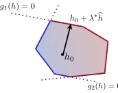
Figure 2: (a) Hypotheses obtained by training on source (green circles), target (red trian-gles) and using DM (dashed blue) and GDM algorithms (solid blue). (b) Objective functions for source and target distribution as well as GDM and DM algorithms. Sets H and surrogate hypothesis set H00 ⊆ H are shown at the bottom. The
vertical lines represent the minimizing hypothesis for each loss.
(2006): the source domain examples were sampled from the uniform distribution over the interval [.2,1] and target ones sampled uniformly over [0, .25]. The labels were given by the map x7→ −x+x3+ξ, where ξ is a Gaussian random variable with mean 0 and standard deviation 0.1. Our hypothesis set was defined by the family of linear functions without an offset. Figure 2(a) shows the regression hypotheses obtained by training the DM and GDM algorithm as well as those obtained by training on the source and target distributions. The ideal hypothesis is shown in red. Notice how the GDM solution gives a closer approximation than DM to the ideal solution. In order to better understand the difference between the solutions of these algorithms, Figure 2(b) depicts the objective function minimized by each algorithm as a function of the slope w of the linear function, the only variable of the hypothesis. The vertical lines show the value of the minimizing hypothesis for each loss. Keeping in mind that the regularization parameter λ used in ridge regression corresponds to a Lagrange multiplier for the constraint w2 ≤Λ2 for some Λ (Cortes and Mohri, 2013) [Lemma 1], the hypothesis set H = {w|w2 ≤ Λ2} is depicted at the bottom of this plot. The shaded region represents the set H00 =H∩ {h00|Lqmin(h
00) ≤ r}. It is clear from this
plot that DM helps approximate the target loss function. Nevertheless, only GDM seems to uniformly approach it. This should come as no surprise since our algorithm was precisely designed to achieve that.
6.2. Adaptation Data Sets
We now present the results of evaluating our algorithm against several other adaptation algorithms. GDM is compared against DM and training on the uniform distribution. The following baselines were also used:
1. The KMM algorithm (Huang et al., 2006), which reweights examples from the source distribution in order to match the mean of the source and target data in a feature space induced by a universal kernel. The hyper-parameters of this algorithm were set to the recommended values ofB = 1000 and=
√
m
√
m−1 .
0.0
0.5
1.0
1.5
2.0
2.5
3.0
3.5
MSE
Source distribution: kin−8fh
0.0
0.5
1.0
1.5
2.0
2.5
3.0
3.5
0.0
0.5
1.0
1.5
2.0
2.5
3.0
3.5
0.0
0.5
1.0
1.5
2.0
2.5
3.0
3.5 GDM
DM Unif Target KMM KLIEP FE
kin−8nm kin−8fm kin−8nh
0.0 0.5 1.0 1.5 2.0
0.2
0.4
0.6
0.8
1.0
0.0 0.5 1.0 1.5 2.0
0.2
0.4
0.6
0.8
1.0
DM/GDM
0.0 0.5 1.0 1.5 2.0
0.2
0.4
0.6
0.8
1.0
● ● ●
● ●
●
● ●
●
●
r Λ
● fh to nm fh to fm fh to nh
(a) (b)
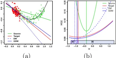
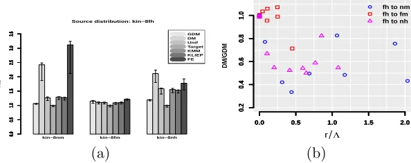
Figure 3: (a)MSE performance for different adaptation algorithms when adapting from
kin-8fh to the three other kin-8xy domains. (b) Relative error of DM over GDM as a function of the ratio r
Λ.
learning the mixture coefficients from the data. Gaussian kernels were used as basis functions for this algorithm and KMM. The bandwidth for the kernel was selected from the set σd:σ= 2−5, . . . ,25 via validation on thetest set, where dis the mean distance between points sampled from the source domain.
3. FE (Daum´e III, 2007). This algorithm maps source and target data into a common high-dimensional feature space where the difference of the distributions is expected to reduce.
Since the two-stage algorithm of Bickel et al. (2007) was already shown to perform similarly to KMM and KLIEP (Cortes and Mohri, 2013), for the sake of readability of our results, we omitted the results of comparison with this algorithm. Finally, we compare our algorithm with the ideal hypothesis h∗ returned by training on the target sample T, which we denote by Tar. Notice that in practice, this is impossible as T is unlabeled so we use
this result only to show the best attainable performance.
We selected the set of linear functions as our hypothesis set. The learning algorithm used for all tasks was ridge regression and the performance evaluated by the mean squared error. We follow the setup of Cortes and Mohri (2011) and for all adaptation algorithms we selected the parameter λvia 10-fold cross validation over the training data by using a grid search over the set of values λ∈ {2−10, . . . ,210}. The results of training on the target distribution are presented for a parameter λ tuned via 10-fold cross validation over the target data. We used the QP implementation of our algorithm with the sampling set H00
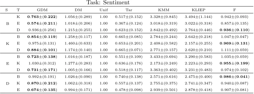
Task: Sentiment
S T GDM DM Unif Tar KMM KLIEP F
B
K 0.763±(0.222) 1.056±(0.289) 1.00 0.517±(0.152) 3.328±(0.845) 3.494±(1.144) 0.942±(0.093)
E 0.574±(0.211) 1.018±(0.206) 1.00 0.367±(0.124) 3.018±(0.319) 3.022±(0.318) 0.857±(0.135)
D 0.936±(0.256) 1.215±(0.255) 1.00 0.623±(0.152) 2.842±(0.492) 2.764±(0.446) 0.936±(0.110)
K
B 0.854±(0.119) 1.258±(0.117) 1.00 0.665±(0.085) 2.784±(0.244) 2.642±(0.218) 1.047±(0.047)
E 0.975±(0.131) 1.460±(0.633) 1.00 0.653±(0.201) 2.408±(0.582) 2.157±(0.255) 0.969±(0.131)
D 0.884±(0.101) 1.174±(0.140) 1.00 0.665±(0.071) 2.771±(0.157) 2.620±(0.210) 1.111±(0.059)
E
B 0.723±(0.138) 1.016±(0.187) 1.00 0.551±(0.109) 3.433±(0.694) 3.290±(0.583) 1.035±(0.059)
K 1.030±(0.312) 1.277±(0.283) 1.00 0.636±(0.176) 2.173±(0.249) 2.223±(0.293) 0.955±(0.199)
D 0.731±(0.171) 1.005±(0.166) 1.00 0.518±(0.117) 3.363±(0.402) 3.231±(0.483) 0.974±(0.102)
D
B 0.992±(0.191) 1.026±(0.090) 1.00 0.740±(0.138) 2.571±(0.616) 2.475±(0.400) 0.986±(0.041)
K 0.870±(0.212) 1.062±(0.318) 1.00 0.557±(0.137) 2.755±(0.375) 2.741±(0.347) 0.940±(0.087)
E 0.674±(0.135) 0.994±(0.171) 1.00 0.478±(0.098) 2.939±(0.501) 2.878±(0.418) 0.907±(0.081)
Table 2: Adaptation from books (B), kitchen (K), electronics (E) and dvd (D) to all
other domains. Normalized results: MSE of training on the unweighted source data is equal to 1. Results in bold represent the algorithm with the lowest MSE.
The first task we considered is given by the 4 kin-8xy Delve data sets (Rasmussen et al., 1996). These data sets are variations of the same model: a realistic simulation of the forward dynamics of an 8 link all-revolute robot arm. The task in all data sets consists of predicting the distance of the end-effector from a target. The data sets differ by the degree of non-linearity (fairly linear,x=f, or non-linear,x=n) and the amount of noise in the output
(moderate, y=m, or high, y=h). The data set defines 4 different domains, that is 12 pairs
of different distributions and labeling functions. A sample of 200 points from each domain was used for training and 10 labeled points from the target distribution were used to select
H00. The experiment was carried out 10 times and the results of testing on a sample of 400 points from the target domain are reported in Figure 3(a). The bars represent the median performance of each algorithm. The error bars are the low and high 25% quartiles respectively. All results were normalized in such a way that the median performance of training on the source is equal to 1. Notice that the performance of all algorithms is comparable when adapting to kin8-fm since both labeling functions are fairly linear, yet
only GDM is able to reasonably adapt to the two data sets with different labeling functions. In order to better understand the advantages of GDM over DM we plot the relative error of DM against GDM as a function of the ratio r/Λ in Figure 3(b), where r is the radius defining H00 and is selected through cross validation. Notice that when the ratio r/Λ is small then both algorithms behave similarly which is most of the times for the adaptation taskfhtofm. On the other hand, a better performance of GDM can be obtained when the
ratio is larger. This is due to the fact that r/Λ measures the effective size of the set H00. A small ratio means that the size ofH00 is small and therefore the hypothesis returned by GDM will be close to that of DM where as if H00 is large then GDM has the possibility of
finding a better hypothesis.
For our next experiment we considered the cross-domain sentiment analysis data set of Blitzer et al. (2007). This data set consists of consumer reviews from 4 different domains:
Task: Images
S T GDM DM Unif Tar KMM KLIEP F
C
I 0.927±(0.051) 1.005±(0.010) 1.00 0.879±(0.048) 2.752±(3.820) 0.936±(0.016) 0.959±(0.035)
S 0.938±(0.064) 0.993±(0.018) 1.00 0.840±(0.057) 0.827±(0.017) 0.835±(0.020) 0.947±(0.025)
B 0.909±(0.040) 1.003±(0.013) 1.00 0.886±(0.052) 0.945±(0.022) 0.942±(0.017) 0.947±(0.019)
I
C 1.011±(0.015) 0.951±(0.011) 1.00 0.802±(0.040) 0.989±(0.036) 1.009±(0.042) 0.971±(0.024)
S 1.006±(0.030) 0.992±(0.016) 1.00 0.871±(0.030) 0.930±(0.018) 0.936±(0.016) 0.973±(0.017)
B 0.987±(0.022) 1.009±(0.010) 1.00 0.986±(0.028) 1.011±(0.028) 1.011±(0.028) 0.994±(0.018)
S
C 1.022±(0.037) 0.982±(0.035) 1.00 0.759±(0.033) 1.172±(0.043) 1.201±(0.038) 0.938±(0.036)
I 0.924±(0.049) 0.998±(0.030) 1.00 0.831±(0.047) 3.868±(4.231) 1.227±(0.039) 0.947±(0.028)
B 0.898±(0.072) 1.003±(0.044) 1.00 0.821±(0.053) 1.240±(0.039) 1.248±(0.041) 0.945±(0.021)
B
C 1.010±(0.014) 0.956±(0.017) 1.00 0.777±(0.031) 1.028±(0.033) 1.032±(0.031) 0.980±(0.019)
I 1.012±(0.010) 1.004±(0.007) 1.00 0.966±(0.009) 2.785±(3.803) 0.981±(0.018) 1.000±(0.004)
S 1.009±(0.018) 0.988±(0.010) 1.00 0.850±(0.035) 0.930±(0.022) 0.934±(0.024) 0.983±(0.013)
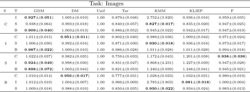
Table 3: Adaptation fromcaltech256 (C),imagenet(I), sun(S) andbing (B).
as the features for this task. For each pair of adaptation tasks we sampled 700 points from the source distribution and 700 unlabeled points from the target. Only 50 labeled points from the target distribution were used to tune the parameterr of our algorithm. The final evaluation is done on a test set of 1000 points. The mean results and standard deviations of this task are shown in Table 2 where the MSE values have been normalized in such a way that the performance of training on the source without reweighting is always 1.
Finally, we considered a novel domain adaptation task (Tommasi et al., 2014) of paramount importance in the computer vision community. The domains correspond to 4 well known collections of images: bing, caltech256, sun and imagenet. These data
sets have been standardized so that they all share the same feature representation and la-beling function (Tommasi et al., 2014). We sampled 800 labeled points from the source distribution and 800 unlabeled points from the target distribution as well as 50 labeled target points to be used for validation of r. The results of testing on 1000 points from the target domain are presented in Table 3 where, again, the results were normalized in such a way that the performance of training on the source data is always 1.
After analyzing the results of this section we notice that the GDM algorithm consis-tently outperforms DM and achieves similar or better performance than all other common adaptation algorithms. It is worth noticing that in some cases, other algorithms perform even worse than training on the unweighted sample. This deficiency of the KLIEP algo-rithm had already been pointed out by Sugiyama et al. (2007) but here we observe that this problem can also affect the KMM algorithm. Finally, let us point out that even though the FE algorithm also achieved performances similar to GDM on the sentiment and image adaptation, its performance was far from optimal adapting on the kin-8xy task. Since there is a lack of theoretical understanding for this algorithm, it is hard to characterize the scenarios where FE would perform better than GDM.
7. Conclusion
so-lution for the particular case of the L2 loss which can be solved in polynomial time. Our empirical results show that our new algorithm always performs better than or is on par with the otherwise state-of-the-art DM algorithm. We also provided tight generalization bounds for the domain adaptation problem based on the Y-discrepancy. As pointed out in Section 4, an algorithm that minimizes the Y-discrepancy would benefit from the best possible guarantees. However, the lack of labeled data from the target distribution makes this algorithm not viable. This suggests analyzing a richer scenario where the learner is allowed to ask for a limited number of labels from the target distribution. This setup, which is related to active learning, seems to be in fact the closest one to real-life applications and has started to receive attention from the research community (Berlind and Urner, 2015). We believe that the discrepancy disc will play a central role in the analysis of that scenario as well.
Acknowledgments
We would like to thank the reviewers of KDD and JMLR for their suggestions to improve this paper. This work was partly funded by the NSF awards IIS-1117591 and CCF-1535987.
Appendix A. SDP Formulation
Lemma 19 The Lagrangian dual of the problem
max
a∈Rm kKsa−yk2≤r2
1
2kKstak
2−b>K
tKsta, (26)
is given by
min
η≥0,γ γ
s. t. − 1 2K
>
stKst+ηK2s 12K
>
stKtb−ηKsy
1 2b
>K
tKst−ηy>Ks η(kyk2−r2) +γ
! 0.
Furthermore, the duality gap for these problems is zero.
Proof For η≥0 the Lagrangian of (26) is given by
L(a, η) = 1
2kKstak
2−b>K
tKsta−η(kKsa−yk2−r2)
=a>1 2K
>
stKst−ηK2s
a+ (2ηKsy−K>stKtb)>a−η(kyk2−r2).
Since the Lagrangian is a quadratic function of a and that the conjugate function of a quadratic can be expressed in terms of the pseudo-inverse, the dual is given by
min
η≥0 1
4(2ηKsy−K
>
stKtb)>
ηK2s−1 2K
>
stKst
†
(2ηKsy−K>stKtb)−η(kyk2−r2)
s. t. ηK2s−1 2K
>
Introducing the variableγ to replace the objective function yields the equivalent problem min
η≥0,γγ
s. t. ηK2s−1 2K
>
stKst 0 γ−1
4(2ηKsy−K
>
stKtb)>
ηK2s−1 2K
>
stKst
†
(2ηKsy−K>stKtb) +η(kyk2−r2)≥0
Finally, by the properties of the Schur complement (Boyd and Vandenberghe, 2004), the two constraints above are equivalent to
−12K>stKst+ηK2s 12K
>
stKtb−ηKsy
1 2K
>
stKtb−ηKsy
>
η(kyk2−r) +γ !
0.
Since duality holds for a general QCQP with only one constraint (Boyd and Vandenberghe, 2004)[Appendix B], the duality gap between these problems is 0.
Proposition 20 The optimization problem (23) is equivalent to the following SDP: max
α,β,ν,Z,z
1 2Tr(K
>
stKstZ)−β−α
s. t νK 2
s+12K
>
stKst− 14Ke νKsy+14Kze νy>Ks+14z>Ke α+ν(kyk2−r2)
!
0 ∧
Z z
z> 1
0
λKt+K2t 12KtKstz 1
2z
>K>
stKt β
!
0 ∧ Tr(K2sZ)−2y>Ksz+kyk2 ≤r2 ∧ ν ≥0,
where Ke =K>stKt(λKt+K2t)†KtKst.
Proof
By Lemma 16, we may rewrite (23) as min
a,γ,η,bb
>(λK
t+K2t)b+
1 2a
>K>
stKsta−a>K>stKtb+γ (27)
s. t. − 1 2K
>
stKst+ηK2s 12K
>
stKtb−ηKsy
1 2b
>K
tKst−ηy>Ks η(kyk2−r2) +γ
!
∧ η ≥0 kKsa−yk2 ≤r2.
Let us apply the change of variablesb= 12(λKt+K2t)†KtKsta+v. The following equalities
can be easily verified. b>(λKt+K2t)b=
1 4a
>K>
stKt(λKt+K2t)†KtKsta+v>KtKsta+v>(λKt+K2t)v.
a>K>stKtb=
1 2a
>
K>stKt(λKt+K2t)
†
Thus, replacingb on (27) yields min
a,v,γ,ηv
>
(λKt+K2t)v+ a
>1
2K
>
stKst−
1 4Ke
a+γ
s. t. −
1 2K
>
stKst+ηK2s 14Kae + 1 2K
>
stKtv−ηKsy
1 4a
>Ke +1 2v
>K
tKst−ηy>Ks η(kyk2−r2) +γ
!
0 ∧ η≥0 kKsa−yk2 ≤r2.
Introducing the scalar multipliers µ, ν ≥0 and the matrix
Z z
z> ez,
0
as a multiplier for the matrix constraint, we can form the Lagrangian:
L:=v>(λKt+K2t)v+a>
1 2K
>
stKst−
1 4Ke
a+γ−µη+ν(kKsa−yk2−r2)
−Tr Zz zze
−1 2K
>
stKst+ηK2s 14Kae + 1 2K
>
stKtv−ηKsy
1 4a
>Ke +1 2v
>K
tKst−ηy>Ks η(kyk2−r2) +γ
!!
.
The KKT conditions ∂∂ηL = ∂∂γL = 0 trivially implyze= 1 and Tr(K2
sZ)−2y>Ksz+kyk2− r2+µ= 0. These constraints on the dual variables guarantee that the primal variablesη and γ will vanish from the Lagrangian, thus yielding
L= 1 2Tr(K
>
stKstZ) +ν(kyk2−r2) +v>(λKt+K2t)v
>−
z>K>stKtv
+a>νK2s+1 2K
>
stKst−
1 4Ke
a−2νKsy+
1 2Kze
>
a.
This is a quadratic function on the primal variablesa and vwith minimizing solutions a= 1
2
νK2s+1 2K
>
stKst−
1 4Ke
†
2νKsy+
1 2Kze
and v= 1
2(λKt+K 2
t)
†
KtKstz,
and optimal value equal to the objective of the Lagrangian dual: 1
2Tr(K
>
stKstZ) +ν(kyk2−r2)−
1 4z >e Kz −1 4
2νKsy+
1 2Kze
>
νK2s+ 1 2K
>
stKst−
1 4Ke
†
2νKsy+
1 2Kze
.
As in Lemma 16, we apply the properties of the Schur complement to show that the dual is given by
max
α,β,ν,Z,z
1 2Tr(K
>
stKstZ)−β−α
s. t νK 2
s+12K
>
stKst−14Ke νKsy+14Kze νy>Ks+ 14z>Ke α+ν(kyk2−r2)
!
0 ∧
Z z
z> 1
0
Tr(K2sZ)−2y>Ksz+kyk2 ≤r2 ∧ β≥
1 4z
>e