Confidence intervals construction for difference of two means with incomplete correlated data

R E S E A R C H A R T I C L E

Open Access

Confidence intervals construction for

difference of two means with incomplete

correlated data

Hui-Qiong Li

1*

, Nian-Sheng Tang

1

and Jie-Yi Yi

2

Abstract

Background:

Incomplete data often arise in various clinical trials such as crossover trials, equivalence trials, and pre

and post-test comparative studies. Various methods have been developed to construct confidence interval (CI) of risk

difference or risk ratio for incomplete paired binary data. But, there is little works done on incomplete continuous

correlated data. To this end, this manuscript aims to develop several approaches to construct CI of the difference of

two means for incomplete continuous correlated data.

Methods:

Large sample method, hybrid method, simple Bootstrap-resampling method based on the maximum

likelihood estimates (

B

1

) and Ekbohm’s unbiased estimator (

B

2

), and percentile Bootstrap-resampling method based

on the maximum likelihood estimates (

B

3

) and Ekbohm’s unbiased estimator (

B

4

) are presented to construct CI of the

difference of two means for incomplete continuous correlated data. Simulation studies are conducted to evaluate the

performance of the proposed CIs in terms of empirical coverage probability, expected interval width, and mesial and

distal non-coverage probabilities.

Results:

Empirical results show that the Bootstrap-resampling-based CIs

B

1

,

B

2

,

B

4

behave satisfactorily for small to

moderate sample sizes in the sense that their coverage probabilities could be well controlled around the

pre-specified nominal confidence level and the ratio of their mesial non-coverage probabilities to the non-coverage

probabilities could be well controlled in the interval [0.4, 0.6].

Conclusions:

If one would like a CI with the shortest interval width, the Bootstrap-resampling-based CIs

B

1

is the

optimal choice.

Keywords:

Bootstrap, Confidence interval, Correlated data, Incomplete data

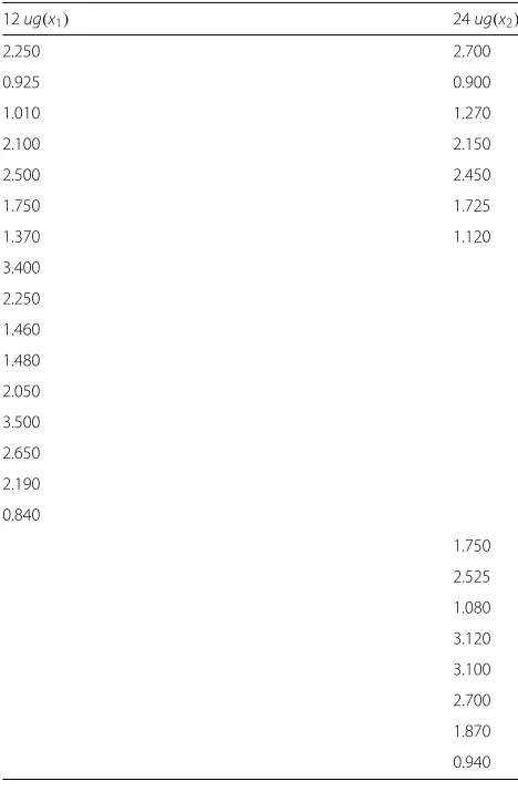
Background

Incomplete data often arise in various research fields

such as crossover trials, equivalence trials, and pre and

post-test comparative studies. For instance, ([1] pp. 212)

designed a crossover clinical trial to measure the onset

of action of two doses of formoterol solution aerosol:

12 ug and 24 ug. In this study, twenty-four patients were

randomly allocated in equal numbers to one of the six

pos-sible sequences of two treatments at a time. Each patient

was received two aerosols at each of visits 2 and 4. After

four weeks, researchers measured the forced expiratory

*Correspondence: [email protected]

1Department of Statistics, Yunnan University, No.2 Cuihu North Road, 650091 Kunming, China

Full list of author information is available at the end of the article

volume of a second (FEV

1

) indicators for twenty-four

patients. Due to the fact that researches did not

con-sider all possible combinations of three treatments (e.g.,

placebo, 12 ug and 24 ug aerosols), which indicates that

the missing data mechanism is missing completely at

ran-dom (MCAR) thus FEV

1

was only observed for 7 patients

under both treatments (e.g., 12 ug and 24 ug aerosols), 9

patients only for 12 ug aerosol, and 8 patients only for 24

ug aerosol. The resultant data are shown in Table 1, which

consist of two parts: the complete observations and the

incomplete observations.

For the above crossover clinical trial, our main

interest is to test the equivalence between 12 ug

and 24 ug formoterol solution aerosols with respect

to the FEV

1

value. To this end, we can

con-struct a

(

1

−

α)

100 % confidence interval for the

Table 1FEV1indicators of patients for 12 ug and 24 ug formoterol solution aerosol

12ug(x1) 24ug(x2)

2.250 2.700

0.925 0.900

1.010 1.270

2.100 2.150

2.500 2.450

1.750 1.725

1.370 1.120

3.400

2.250

1.460

1.480

2.050

3.500

2.650

2.190

0.840

1.750

2.525

1.080

3.120

3.100

2.700

1.870

0.940

difference of two FEV

1

values. If the resultant

confidence interval (CI) lies entirely in the interval

(

−

δ

0

,

δ

0

)

with

δ

0

(>

0

)

being some pre-specified clinical

acceptable threshold, we thus could conclude the

equiva-lence between two doses of formoterol solution aerosol at

the

α

significance level. As a result, reliable CIs for the

diff-erence in the presence of incomplete data are necessary.

The problem of testing the equality and constructing

CI for the difference of two correlated proportions in the

presence of incomplete paired binary data has received

considerable attention in past years. For example, ones

can refer to [2–6] for the large sample method, and [7]

for the corrected profile likelihood method. When

sam-ple size is small, [8] proposed the exact unconditional test

procedure for testing equality of two correlated

propor-tions with incomplete correlated data. Tang, Ling and Tian

[9] developed the exact unconditional and approximate

unconditional CIs for proportion difference in the

pres-ence of incomplete paired binary data. Lin et al. [10]

presented a Bayesian method to test equality of two

correlated proportions with incomplete correlated data.

Li et al. [11] discussed the confidence interval

con-struction for rate ratio in matched-pair studies with

incomplete data. However, all the aforementioned

meth-ods were developed for incomplete paired binary data.

Statistical inference on the difference of two means

with incomplete correlated data has received a limited

attention. For example, [12] discussed the problem of

test-ing the equality of two means with misstest-ing data on one

response and recommended [13] statistic when the

vari-ances were not too different. Lin and Stivers [14] also gave

a similar comparison. Lin and Stivers [15] and [12]

sug-gested some test statistics for testing the equality of two

means with incomplete data on both response. However,

to our knowledge, little work has been done on CI

con-struction for the difference of two means with incomplete

correlated data under the MCAR assumption.

Inspired by [16–19], we develop several CIs for the

dif-ference of two means with incomplete correlated data

under the MCAR assumption based on the large

sam-ple method, hybrid method and Bootstrap-resampling

method. The presented Bootstrap-resampling CIs have

not been considered in the literature related to missing

observations.

The rest of this article is organized as follows. Several

methods are presented to construct CIs for the

differ-ence of the two means with incomplete correlated data

in Section “Methods”. Simulation studies and an example

are conducted to evaluate the finite performance of the

proposed CIs in terms of coverage probability, expected

interval width, and mesial and distal non-coverage

prob-abilities in Section “Results”. A brief discussion is given in

Section “Discussion”. Some concluding remarks are given

in Section “Conclusion”.

Methods

Suppose that

x

=

(

x1

,

x2

)

is a 2

×

1 vector of random

variables, and follows a distribution with mean

μ

and

covariance matrix

given by

μ

=

μ

1

μ

2

and

=

σ

2

1

ρσ

1

σ

2

ρσ

1

σ

2

σ

22

,

respectively. Let

{

(

x

1m

,

x

2m

)

:

m

=

1,

· · ·

,

n

}

be

n

paired

observations on

x

1

and

x

2

,

x

1,n+1

,

· · ·

,

x

1,n+n1

be

n

1

additional observations on

x

1

,

x

2,n+1

,

· · ·

,

x

2,n+n2

be

n

2

additional observations on

x

2

. Thus, there are

n

1

missing

observations on

x2, and

n2

missing observations on

x1.

Without loss of generality, the data may be presented as

follows:

x11,

· · ·

,

x1

n

,

x1,

n+1,

· · ·

,

x1,

n+n1

,

x21,

· · ·

,

x2

n

,

x2,

n+1,

· · ·

,

x2,

n+n2

,

is MCAR (i.e., independent of treatment and outcome).

Based on these observations, we here want to construct

reliable explicit CIs for the difference of two means

δ

=

μ

1

−

μ

2

under MCAR assumption.

Confidence interval based on the large sample method

To make a comparison with the following proposed

methods, we assume that

x

follows a bivariate normal

dis-tribution in this subsection. In this case, if only variable

x

1

or

x

2

is subject to missingness (i.e.,

n

1

=

0 or

n

2

=

0), one

can obtain the closed forms of the maximum likelihood

estimates (MLEs) of

μ

and

[22]. However, there are no

closed forms of the MLEs for

μ

and

when variables

x

1

and

x

2

are simultaneously subject to missingness (i.e.,

n

1

=

0 and

n

2

=

0), though one can find the MLEs of

μ

and

using an iterative algorithm [23]. To get the closed

forms of MLEs for

μ

and

, [15] proposed the modified

MLEs using a non-iterative procedure and provided

sev-eral test statistics based on the obtained estimators of

μ

and

.

(i) Confidence interval based on Lin and Stivers’s test

statistics

Let

δ

ˆ

= ˆ

μ

1

− ˆ

μ

2

be the MLE of

δ

under the bivariate

nor-mal assumption of

x

. When

is known, it follows from

[15] that the MLE of

δ

is

ˆ

δ

=

ax

(₁n)

+

(

1

−

a

)

x

(n1)

1

−

bx

( n)

2

−

(

1

−

b

)

x

( n2)

2

,

and the asymptotic variance of

δ

ˆ

can be expressed as

Var

(

δ)

ˆ

=

h

n

+

n

2

(

1

−

ρ)

2

σ

2

1

−

2n

ρσ

1

σ

2

+

n

+

n1

1

−

ρ

2

σ

₂2

,

respectively, where

x

(₁n)

=

1_n

n_j=1

x

1j

,

x

(2n)

=

1n

n

j=1

x

2j

,

x

(n1)

1

=

n11

n1

j=1

x1,

n+j

,

x

(n2)

2

=

n12

n2

k=1

x

2,n+k

,

a

=

nh

(

n

+

n2

+

n1

β

21

)

,

b

=

nh

(

n

+

n1

+

n2

β

12

)

,

β

21

=

ρσ

2

/σ

1

,

β

12

=

ρσ

1

/σ

2

,

h

=

1

/

{

(

n

+

n

1

)(

n

+

n

2

)

−

n

1

n

2

ρ

2

}

. An approximate 100

(

1

−

α)

% CI of

δ

is given by

ˆ

δ

−

z

α/2

Var

(

δ)

ˆ

,

δ

ˆ

+

z

α/2

Var

(

δ)

ˆ

, which is denoted as

T

w1

-CI.

Following [15], when

is unknown, the statistic for

testing

H

0

:

δ

=

δ

0

versus

H

1

:

δ

=

δ

0

is given by

T

1

=

A

x

(₁n)

−

x

(n1)

1

−

B

x

(₂n)

−

x

(n2)

2

+

x

(n1)

1

−

x

(n2)

2

−

δ

0

√

V

1

,

which is asymptotically distributed as

t-distribution

with

n

degrees of freedom under

H

0

, where

V

1

=

{

A

2

_/

_n

₊

₍

₁

₋

_A

₎

2

_/

_n

1

}

m

1

+ {

B

2

/

n

+

(

1

−

B

)

2

/

n

2

}

m

2

−

2ABm

12

/

n]

/(

n

−

1

)

,

A

= {

n

(

n

+

n

2

+

n

1

m

12

/

m

1

}

/

(

n

+

n

1

)(

n

+

n

2

)

−

n

1

n

2

r

2

−1

,

B

= {

n

(

n

+

n

1

+

n

2

m

12

/

m

2

}

/

(

n

+

n

1

)(

n

+

n

2

)

−

n

1

n

2

r

2

−1

,

m

1

=

nj=1

x

1j

−

x

(1n)

2

,

m

2

=

nj=1

x

2j

−

x

(2n)

2

,

m

12

=

nj=1

x

1j−

x

(1n)

x

2j

−

x

(2n)

,

r

=

m

12

/

√

m

1

m

2

. Therefore, the

approximate 100

(

1

−

α)

% CI on the basis of

T

1

is given

by (L,

U), where

L

=

A

x

₁(n)

−

x

(n1)

1

−

B

x

(₂n)

−

x

(n2)

2

+

x

(n1)

1

−

x

(

n2)

2

−

t

α/2

(

n

)

√

V

1

, and

U

=

A

x

(₁n)

−

x

(n1)

1

−

B

x

(₂n)

−

x

(n2)

2

+

x

(n1)

1

−

x

(

n2)

2

+

t

α/2

(

n

)

√

V

1

, which is

denoted as

T

1

-CI.

Another test statistic defined by [15] for testing

H

0

:

δ

=

δ

0

versus

H

1

:

δ

=

δ

0

, which is a generalization of [24] test

statistic for two independent samples, is given by

T

2

=

¯

x

(n+n1)

1

− ¯

x

( n+n2)

2

−

δ

0

√

h

1

+

h

2

+

h

3

,

which is asymptotically distributed as

t

distribu-tion with degrees

ν

of freedom, where

x

¯

(n+n1)

1

=

(

n

+

n

1

)

−1

jn=+1n1

x

1j

,

x

¯

2(n+n2)

=

(

n

+

n

2

)

−1

jn=+1n2

x

2j

,

h

1

=

n

{

(

n

+

n

2

)

m

1

/(

n

+

n

1

)

+

(

n

+

n

1

)

m

2

/(

n

+

n

2

)

−

2m

12

}

/

{

(

n

−

1

)(

n

+

n

1

)(

n

+

n

2

)

}

,

h

2

=

n

1

b

1

/

{

(

n

1

−

1

) (

n

+

n

1

)

2

}

,

h3

=

n2b2

/

{

(

n2

−

1

)(

n

+

n2

)

2

}

,

b1

=

n+n1

j=n+1

x

1j

−

x

(1n1)

2

,

b

2

=

nj=+nn+21

x

2j

−

x

(2n1)

2

, and

ν

=

(

h1

+

h2

+

h3

)

2

/

{

h

2₁

/(

n

−

1

)

+

h

2₂

/(

n1

−

1

)

+

h

2₃

/(

n2

−

1

)

}

.

Therefore, the approximate 100

(

1

−

α)

% CI of

δ

for

statistic

T

2

is denoted as

T

2

-CI.

When

σ

1

=

σ

2

, it follows from [15] that the statistic for

testing

H

0

:

δ

=

δ

0

versus

H

1

:

δ

=

δ

0

can be expressed as

T3=

¯

x(n+n1)

1 − ¯x(

n+n2)

2 −δ0

_{(n+n1+n2−2)(n+n1)(n+n2)}

(b1+c2)(2n−2nr+n1+n2) ,

which is asymptotically distribution as

t-distribution with

degrees

n

+

n

1

+

n

2

−

4 of freedom. Note that when

n2

>

n1,

b1

+

c2

should be replaced by

b2

+

c1. Thus,

the approximate 100

(

1

−

α)

% CI of

δ

for

T3

is denoted as

T

3

-CI, where

c

1

=

nj=+1n1

x

1j

−

n

+

n

1

jn=+1n1

x

1j

2

, and

c

2

=

nj=+1n2

x

2j

−

_n+1_n2

jn=+1n2

x

2j

2

.

Also, [12] presented the similar but simpler test

statis-tics for testing the mean difference

δ

=

μ

1

−

μ

2

, which are

adopted to construct CIs of

δ

as follows.

(ii) Confidence interval based on Ekbohm’s test statistics

Following [12], an unbiased estimator of

δ

is given

by

δ

ˆ

=

x

¯

(n+n1)

1

− ¯

x

(n+n2)

2

, and its variance is

given by Var

(

δ)

ˆ

=

Var

(

μ)

ˆ

=

(

n

+

n

2

)σ

12

+

(

n

+

n

2

)σ

22

−

2n

ρσ

1

σ

2

}

/

{

(

n

+

n1

)(

n

+

n2

)

}

. An approximate 100

(

1

−

α)

% CI of

δ

can be obtained by

ˆ

δ

−

z

α/2

Var

(

δ)

ˆ

,

δ

ˆ

+

z

α/2

Var

(

δ)

ˆ

When

σ

1

=

σ

2

, Ekbothm (1976) proposed the following statistic for testing

H

0

:

T

4

=

(

δ

˜

−

δ

0

)

(

n

+

n

1

)(

n

+

n

2

)

−

n

1

n

2

λ

2

/

ˆ

σ

2n

(

1

−

λ)

+

(

n1

+

n2

)(

1

−

λ

2

₎

_{, where}

_δ

˜

₌

_n

₍

_n

₊

_n2

₊

_n1

_λ)

_x

(n)

1

−

n

(

n

+

n1

+

n2

λ)

x

(n) 2

+

n1

n

+

n2

1

−

λ

2

−

n

λ

}

x

(n1)

1

−

n2

n

+

n1

(

1

−

λ)

2

−

n

λ

x

(n2)

2

(

n

+

n1

)(

n

+

n2

)

−

n1n2

λ

2

,

σ

ˆ

2

=

m1

+

m2

+

(

1

+

λ

2

)(

b1

+

b2

)

/

{

2

(

n

−

1

)

+

(

1

+

λ

2

)(

n

1

+

n

2

−

2

)

, and

λ

=

2m

12

/(

m

1

+

m

2

)

. Under

H

0

,

T

4

is asymptotically distributed as

t-distribution with degrees

n

of freedom. Therefore, the approximate 100

(

1

−

α)

% CI is denoted as

T

4

-CI.

Following [12], when

σ

1

=

σ

2, another statistic for testing

H0

can be expressed as

T5

=

¯

x

(n+n1)

1

− ¯

x

(n+n2)

2

−

δ

0

√

(

n

+

n

1

)(

n

+

n

2

)/(

R

1

+

R

2

)

, which is asymptotically distributed as

t

distribution with degrees

ν

σ

of freedom under

H

0

, where

R

1

=

n

(

m

1

+

m

2

−

2m

12

) / (

n

−

1

)

,

R

2

=

(

n

1

+

n

2

)(

b

1

+

b

2

)/(

n

1

+

n

2

−

2

)

, and

ν

σ

=

(

R

1

+

R

2

)

2

/

R

2₁

/(

n

+

1

)

+

R

2₂

/(

n

1

+

n

2

)

−

2. Thus, an approximate 100

(

1

−

α)

% CI of

δ

for

T

5

is denoted as

T

5

-CI.

Confidence interval based on the generalized estimating equations(GEEs)

To relax the bivariate normality assumption of

x

, the method of the generalized estimating equations (GEEs) with

exchangeable working correlation structure (e.g., [25]) can be adopted to make statistical inference on

δ

in the

incom-plete correlated data because the GEE approach have become one of the most widely used methods in dealing with

correlated response data [26, 27]. Following [28], the GEEs with exchangeable working correlation structure can be

used to estimate parameter vector

μ

; the so-called sandwich variance estimator can be used to consistently estimate the

covariance matrix of

μ

; and the ML method under a bivariate normal assumption via available paired observations is

used to estimate the correlation parameter. Thus, an approximate 100

(

1

−

α)

% CI of

δ

based on GEE method is denoted

as

T

g

-CI.

Confidence interval based on the hybrid method

When the distribution function of

x

is unknown, a hybrid method is developed to construct CI of

δ

in this subsection.

We first introduce the general concept of hybrid method. Let

θ

1

and

θ

2

be two parameters of interest. Now our main

interest is to construct a 100

(

1

−

α)

% two-sided CI

(

L,

U

)

of

θ

1

−

θ

2

via hybrid method. Let

θ

ˆ

1

and

θ

ˆ

2

be two estimates of

θ

1

and

θ

2

, respectively; and let

(

l

1

,

u

1

)

and

(

l

2

,

u

2

)

denote two approximate 100

(

1

−

α)

% CIs for

θ

1

and

θ

2

, respectively.

Under the dependent assumption on

θ

ˆ

1

and

θ

ˆ

2

, it follows from the central limit theorem that the approximate two-sided

100

(

1

−

α)

% CI of

θ

1

−

θ

2

is given by

(

L,

U

)

, where

L

= ˆ

θ

1

− ˆ

θ

2

−

z

α/2

Var

(

θ

ˆ

1

)

+

Var

(

θ

ˆ

2

)

−

2Cov

(

θ

ˆ

1

,

θ

ˆ

2

)

,

U

= ˆ

θ

1

− ˆ

θ

2

+

z

α/2

Var

(

θ

ˆ

1

)

+

Var

(

θ

ˆ

2

)

−

2Cov

(

θ

ˆ

1

,

θ

ˆ

2

)

.

Because Cov

(

θ

ˆ

1

,

θ

ˆ

2

)

=

corr

(

θ

ˆ

1

,

θ

ˆ

2

)

Var

(

θ

ˆ

1

)

Var

(

θ

ˆ

2

)

1/2

, the lower limit

L

and the upper limit

U

can be rewritten as

L

= ˆ

θ

1

− ˆ

θ

2

−

z

α/2

Var

(

θ

ˆ

1

)

+

Var

(

θ

ˆ

2

)

−

2corr

(

θ

ˆ

1

,

θ

ˆ

2

)

Var

(

θ

ˆ

1

)

Var

(

θ

ˆ

2

)

1/2

U

= ˆ

θ

1

− ˆ

θ

2

+

z

α/2

Var

(

θ

ˆ

1

)

+

Var

(

θ

ˆ

2

)

−

2corr

(

θ

ˆ

1,

θ

ˆ

2

)

Var

(

θ

ˆ

1

)

Var

(

θ

ˆ

2

)

1/2

,

respectively. Note that

(

l

1

,

u

1

)

contains the plausible parameter values of

θ

1

, and

(

l

2

,

u

2

)

contains the plausible parameter

values for

θ

2

. Among these plausible values for

θ

1

and

θ

2

, the values closest to the minimum

L

and maximum

U

are

respectively

l

1

−

u

2

and

u

1

−

l

2

in spirit of the score-type CI [29]. From the central limit theorem, the variance estimates

can now be recovered from

θ

1

=

l1

as

Var

(

θ

ˆ

1

)

=

(

θ

ˆ

1

−

l1

)

2

/

z

2_α/2

and from

θ

2

=

u2

as

Var

(

θ

ˆ

2

)

=

u2

− ˆ

θ

2

2

z

2_α/2

for

setting

L. As a result, the lower limit

L

for

θ

1

−

θ

2

is

L

= ˆ

θ

1

− ˆ

θ

2

−

ˆ

θ

1

−

l1

2

+

u2

− ˆ

θ

2

2

−

2

corr

ˆ

θ

1,

θ

ˆ

2

ˆ

θ

1

−

l1

u2

− ˆ

θ

2

(1)

Similarly, we can obtain

U

= ˆ

θ

1

− ˆ

θ

2

+

u

1

− ˆ

θ

1

2

+

θ

ˆ

2

−

l

2

2

−

2

corr

θ

ˆ

1

,

θ

ˆ

2

u

1

− ˆ

θ

1

ˆ

θ

2

−

l

2

(2)

(i)

The Wilson score method

l

i

= ˜

θ

i

−

z

α/2

N

i

+

z

2_α/2

n

n

−

1

n

j=1

x

ij

− ˆ

θ

i

2

+

z

2 α/2

4

,

u

i

= ˜

θ

i

+

z

α/2

N

i

+

z

2_α/2

n

n

−

1

n

j=1

x

ij

− ˆ

θ

i

2

+

z

2 α/2

4

,

where

N

i

=

n

+

n

i

and

θ

ˆ

i

=

_N1_i

Ni

j=1

x

ij

for

i

=

1, 2.

(ii)The Agresti-coull method

li= ˜θi−zα/2

n

j=1(xij− ˆθi)2

Ni+z_α/22

(n−1)

,

ui= ˜θi+zα/2

n

j=1(xij− ˆθi)2

Ni+z2_α/2

(n−1)

,

where

N

i

=

n

+

n

i

and

θ

˜

i

=

Nj=i1

x

ij

+

0.5z

2_α/2

/

N

i

+

z

2_α/2

for

i

=

1, 2.

To construct CI for

δ

=

μ

1

−

μ

2

via the above described

hybrid method, we can simply set

θ

1

=

μ

1

and

θ

2

=

μ

2

. If

is known, the estimated correlation coefficient

corr

(

μ

ˆ

1

,

μ

ˆ

2

)

of

μ

ˆ

1

and

μ

ˆ

2

is given by

corr

(

μ

ˆ

1

,

μ

ˆ

2

)

=

2n

ρ/

√

(

n

+

n

1

)(

n

+

n

2

)

. If

is unknown,

corr

(

μ

ˆ

1

,

μ

ˆ

2

)

is

given by

corr

(

μ

ˆ

1,

μ

ˆ

2

)

=

nr

/

(

n

+

n1

)(

n

+

n2

)

−

n1n2r

2

,

where

r

=

m

12

/

√

m

1

m

2

,

m

1

=

nj=1

x

1j

−

x

(1n)

2

and

m

2

=

nj=1

x

2j

−

x

(2n)

2

. Thus, using Eqs. (1) and (2)

yields CIs of

δ

=

μ

1

−

μ

2

. When

l

i

and

u

i

are estimated by

the Wilson score method, we denote the corresponding CI

as

W

s

-CI; when

l

i

and

u

i

are estimated by the Agresti-coull

method, the corresponding CI is denoted as

W

a

-CI.

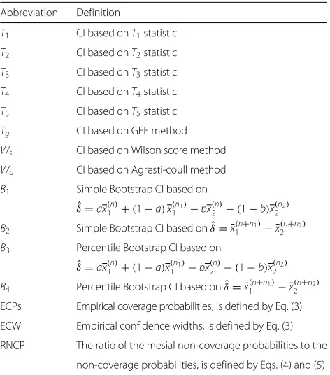
Bootstrap-resampling-based confidence intervals

When the distribution of

x

is known, one can obtain

the approximate CIs of

δ

based on the asymptotic

distri-butions of the constructed test statistics under the null

hypotheses

H

0

:

δ

=

δ

0

. However, when the

distribu-tion of

x

is unknown, the asymptotic distributions of the

constructed test statistics may not be reliable, especially

with small sample size. On the other hand, estimators

of some nuisance parameters have not the closed-form

solutions even if the approximate distribution is reliable,

and they must be obtained by using some iterative

algo-rithms, which are computationally intensive. In this case,

the Bootstrap method is often adopted to construct CIs

of parameter of interest. The Bootstrap CIs can be

con-structed via the following steps.

Step 1.

Given the paired observations and incomplete

observations

D

=

x11,

· · ·

,

x1

n

,

x1,

n+1,

· · ·

,

x1,

n+n1

,

x

21

,

· · ·

,

x

2n

,

x

2,n+1

,

· · ·

,

x

2,n+n2

we draw

n

paired observations

(

x

∗_1m

,

x

∗_2m

)

:

m

=

1,

· · ·

,

n

with replacement from

n

paired observations

{

(

x

11

,

x

21

)

,

· · ·

,

(

x

1n

,

x

2n

)

}

, generate

n

1

observations

{

x

∗1,n+j

:

j

=

1,

· · ·

,

n

1

}

with replacement from

x

1,n+1

,

· · ·

,

x

1,n+n1

,

and sample

n

2

observations

x

∗_2,n+k

:

k

=

1,

· · ·

,

n

2

with

replacement from

x

2,n+1

,

· · ·

,

x

2,n+n1

. Thus, we obtain

the following Bootstrap resampling sample

D

∗_b

=

x∗₁₁,· · ·,x∗_1n, x_1,∗_n+1,· · ·,x∗_1,n+n 1,

x∗₂₁,· · ·,x∗_2n, ,x_2,∗_n+1,· · ·,x∗_2,n+n2

.

Step 2.

For the above generated Bootstrap resampling

sample

D

∗_b

, we first compute

μ

ˆ

∗₁

=

(

n

+

n1

)

−1

n+n1

j=1

x

∗1j

and

μ

ˆ

∗₂

=

(

n

+

n

2

)

−1

nj=+1n2

x

∗2j

, and then calculate the

estimated value

δ

ˆ

∗

of

δ

via

δ

ˆ

∗

= ˆ

μ

∗₁

− ˆ

μ

∗₂

.

Step 3.

Repeating the above steps 1 and 2 for a total of

G

times yields

G

Bootstrap estimates

δ

ˆ

∗_g

:

g

=

1, 2,

· · ·

,

G

of

δ

. Let

δ

ˆ

₍₁₎∗

<

δ

ˆ

₍₂₎

<

· · ·

<

δ

ˆ

₍∗_G)

be the ordered values of

ˆ

δ

∗

g

:

g

=

1, 2,

· · ·

,

G

.

Step 4.

Based on the bootstrap estimates

δ

ˆ

∗_g

,

g

=

1, 2,

. . .

,

G

, Bootstrap-resampling-based CIs for

δ

can be

constructed as follows.

Generally, the standard error se

(

δ)

ˆ

of

δ

ˆ

can be estimated

by the sample standard deviation of the

G

replications,

i.e.,

se

ˆ

(

δ)

ˆ

=

(

G

−

1

)

−1

G g=1

ˆ

δ

∗

g

− ¯

δ

∗B

2

, where

δ¯∗

B =

ˆ

δ∗

1+ · · · + ˆδG∗

/G

. If

δˆ∗

g :g=1,· · ·,G

is approximately

normally distributed, an approximate 100

(

1

−

α)

%

Boot-strap CI for

δ

is given by

δ

ˆ

−

z

_α/2

se

ˆ

(

δ)

ˆ

,

δ

ˆ

+

z

_α/2

se

ˆ

(

δ)

ˆ

,

where

z

α/2

is the upper

α/

2-percentile of the standard

normal distribution, which is referred as the simple

Boot-strap confidence interval. When

δ

ˆ

=

ax

(₁n)

+

(

1

−

a

)

x

(n1)

1

−

bx

(₂n)

−

(

1

−

b

)

x

(n2)

2

, the corresponding simple Bootstrap

CI is denoted as

B

1

. When

δ

ˆ

= ¯

x

1(n+n1)

− ¯

x

(2n+n2)

, the

corresponding simple Bootstrap CI is denoted as

B

2

.

Alternatively, if

δ

ˆ

_g∗

:

g

=

1,

· · ·

,

G

is not normally

dis-tributed, it follows from ([16] p.132) that the approximate

100

(

1

−

α)

% Bootstrap-resampling-based percentile CI

for

δ

is

δˆ∗

([Gα/2]),δˆ(∗[G(1−α/2)])

, where [a] represents the

integer part of

a, which is referred as the percentile

Boot-strap CI. When

δ

ˆ

=

ax

(₁n)

+

(

1

−

a

)

x

(n1)

1

−

bx

(n)

2

−

(

1

−

b

)

x

(n2)

2

, the corresponding percentile Bootstrap CI is

denoted as

B

3

. When

δ

ˆ

= ¯

x

1(n+n1)

− ¯

x

(

n+n2)

2

, the

corre-sponding percentile Bootstrap CI is denoted as

B

4

.

Results

Simulation studies

(ECP), empirical confidence widths (ECW), and distal

and mesial non-coverage probabilities (DNP and MNP)

in various parameter settings via Monte Carlo simulation

studies. A summary of abbreviation for various confidence

intervals is presented in Table 2.

In the first simulation study, we consider the

follow-ing case that

(

n,

n

1

,

n

2

)

is set to be

(

5, 2, 2

)

;

μ

1

=

0, 1, 2;

μ

2

=

0.25, 1, 1.5;

ρ

= −

0.9,

−

0.5,

−

0.1, 0, 0.1, 0.5, 0.9;

δ

=

μ

1

−

μ

2

= −

0.25, 0, 0.5;

σ

22

=

4;

σ

12

=

1, 8 and

α

=

0.05. For a given combination

(

n,

n1,

n2,

μ

1,

μ

2,

ρ

,

σ

1,

σ

2

)

,

we generate

n

+

n1

+

n2

random samples of

(

x1,

x2

)

from

a bivariate normal distribution with

μ

=

(μ

1,

μ

2

)

and

=

σ

2

1

ρσ

1

σ

2

ρσ

1

σ

2

σ

22

.

Then, for the generated

n

+

n

1

+

n

2

random samples,

the

n

1

observations on

x

2

are deleted randomly. For the

remaining paired

n

+

n

2

random samples, the

n

2

obser-vations on

x

1

are deleted randomly. Thus,

(

x

1m

,

x

2m

)

(

m

=

1,

· · ·

,

n

)

are

n

pairs observations on

(

x

1

,

x

2

)

;

x

1,n+j

(

j

=

1,

· · ·

,

n

1

)

are

n

1

additional observations on

x

1

;

x

2,n+k

(

k

=

1,

· · ·

,

n2

)

are

n2

additional observations on

x2. Based on the observation

{

(

x1

j

,

x2

j

)

:

m

=

1,

· · ·

,

n

}

,

{

x1,

n+j

:

j

=

1,

· · ·

,

n1

}

,

{

x

2,n+k

:

k

=

1,

· · ·

,

n2

}

, we can

draw 5000 bootstrap resampling samples. Independently

repeating the above process

M

=

10000 times, we can

compute their corresponding ECP, ECW, MNP and DNP

values. The ECP, ECW, MNP and DNP are defined by

Table 2Summary of various abbreviations

Abbreviation Definition

T1 CI based onT1statistic

T2 CI based onT2statistic

T3 CI based onT3statistic

T4 CI based onT4statistic

T5 CI based onT5statistic

Tg CI based on GEE method

Ws CI based on Wilson score method

Wa CI based on Agresti-coull method

B1 Simple Bootstrap CI based on

ˆ

δ=ax(₁n)₊₍1₋a₎x(n1)

1 −bx( n)

2 −(1−b)x( n2)

2 B2 Simple Bootstrap CI based onδˆ= ¯x1(n+n1)− ¯x(

n+n2)

2 B3 Percentile Bootstrap CI based on

ˆ

δ=ax(₁n)+(1−a)x(n1)

1 −bx( n)

2 −(1−b)x( n2)

2 B4 Percentile Bootstrap CI based onδˆ= ¯x1(n+n1)− ¯x(

n+n2)

2 ECPs Empirical coverage probabilities, is defined by Eq. (3)

ECW Empirical confidence widths, is defined by Eq. (3)

RNCP The ratio of the mesial non-coverage probabilities to the

non-coverage probabilities, is defined by Eqs. (4) and (5)

ECP

=

1

M

M

m=1

I

δ

∈

L

x

(m)

,

U

x

(m)

,

ECW

=

1

M

M

m=1

U

x

(m)

)

−

L

x

(m)

,

(3)

MNP

=

1

M

M

m=1

I

δ

∈

−∞

,

L

x

(m)

,

DNP

=

1

M

M

m=1

I

δ

∈

U

x

(m)

,

+∞

,

(4)

respectively, where

I

{

δ

∈

A

}

is an indicator function,

which is 1 if

δ

∈

A

and 0 otherwise. The

ratio of the MNP

to the non-coverage probability (NCP) is defined as

RNCP

=

MNP

NCP

=

MNP

1.0

−

ECP

.

(5)

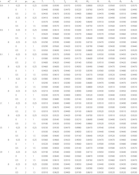
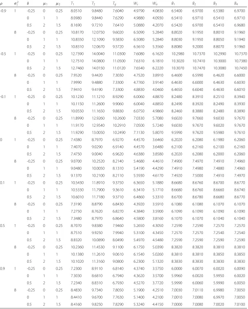
Results are presented in Tables 3, 4 and 5. Also, to

investigate the performance of the proposed CIs under

the assumption

σ

₁2

=

σ

₂2

=

σ

2

_{, we calculate the}

cor-responding results for

T

3

,

T

4

,

T

5

, hybrid CIs,

Bootstrap-resampling-based CIs when

σ

2

₌

_{4 and}

₍

_n,

_n

1

,

n

2

)

=

(

5, 5, 2

)

, which are given in Tables 9, 10 and 11.

Following [17, 30], an interval can be regarded as

sat-isfactory if (i) its ECP is close to the pre-specified 95 %

confidence level, (ii) it possesses shorter interval width,

and (iii) its RNCP lies in the interval [ 0.4, 0.6];

too mesially

located

if its RNCP is less than 0.4; and

too distally

if its

RNCP is greater than 0.6.

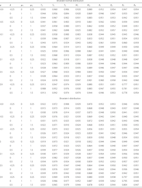
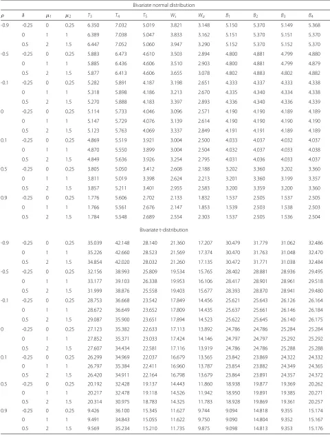
In the second Monte Carlo simulation study, we assume

that the random samples of bivariate variables

x1

and

x2

are generated from a bivariate

t-distribution with five

degrees of freedom, and mean

μ

and scale parameter

specified in the first simulation study. The corresponding

results with

(

n,

n

1

,

n

2

)

=

(

5, 5, 5

)

are given in Tables 6, 7

and 8. Similarly, we calculate the corresponding results for

T

3

,

T

4

,

T

5

, hybrid CIs, Bootstrap-resampling-based CIs

when

σ

2

=

4 and

(

n,

n

1

,

n

2

)

=

(

5, 5, 2

)

, which are given in

Tables 9, 10 and 11.

To investigate powers for the proposed CIs, we

calcu-lated the power in both the first and second simulation

study. The results are shown in Tables 12 and 13. There is

very little power in both the first and second simulation

study to exclude a difference of zero.

Results of simulation studies

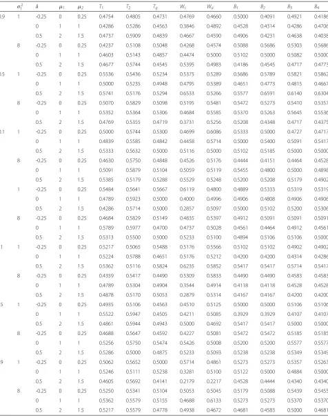
Table 3ECPs of various confidence intervals under bivariate normal distribution with differentρandδ,μ1,μ2σ12and(n,n1,n2)= (5, 2, 2)andσ2

2 =4

ρ σ2

1 δ μ1 μ2 T1 T2 Tg Ws Wa B1 B2 B3 B4

-0.9 1 -0.25 0 0.25 0.9390 0.9590 0.9370 0.9350 0.8800 0.9520 0.9560 0.9370 0.9570

0 1 1 0.9440 0.9580 0.9470 0.9220 0.8760 0.9470 0.9490 0.9300 0.9490

0.5 2 1.5 0.9430 0.9670 0.9530 0.9400 0.8860 0.9470 0.9480 0.9310 0.9480

8 -0.25 0 0.25 0.9410 0.9630 0.9450 0.9180 0.8600 0.9430 0.9490 0.9340 0.9490

0 1 1 0.9370 0.9580 0.9350 0.9240 0.8640 0.9510 0.9500 0.9390 0.9500

0.5 2 1.5 0.9380 0.9570 0.9410 0.9240 0.8750 0.9570 0.9560 0.9470 0.9560

-0.5 1 -0.25 0 0.25 0.9440 0.9610 0.9530 0.9200 0.8570 0.9490 0.9430 0.9330 0.9420

0 1 1 0.9420 0.9660 0.9230 0.9270 0.8660 0.9570 0.9560 0.9460 0.9550

0.5 2 1.5 0.9460 0.9660 0.9380 0.9250 0.8640 0.9480 0.9560 0.9430 0.9540

8 -0.25 0 0.25 0.9290 0.9590 0.9480 0.9230 0.8730 0.9470 0.9450 0.9390 0.9440

0 1 1 0.9290 0.9560 0.9420 0.9210 0.8790 0.9460 0.9430 0.9380 0.9440

0.5 2 1.5 0.9350 0.9690 0.9410 0.9330 0.8880 0.9520 0.9540 0.9470 0.9520

-0.1 1 -0.25 0 0.25 0.9300 0.9570 0.9500 0.9170 0.8630 0.9550 0.9500 0.9450 0.9470

0 1 1 0.9380 0.9590 0.9450 0.9170 0.8600 0.9540 0.9500 0.9450 0.9520

0.5 2 1.5 0.9400 0.9620 0.9440 0.9140 0.8560 0.9510 0.9460 0.9420 0.9460

8 -0.25 0 0.25 0.9460 0.9600 0.9310 0.9050 0.8490 0.9460 0.9470 0.9440 0.9470

0 1 1 0.9450 0.9670 0.9440 0.9150 0.8590 0.9560 0.9500 0.9480 0.9510

0.5 2 1.5 0.9350 0.9610 0.9360 0.9150 0.8570 0.9500 0.9520 0.9440 0.9490

0 1 -0.25 0 0.25 0.9380 0.9610 0.9400 0.9330 0.8860 0.9550 0.9550 0.9530 0.9530

0 1 1 0.9290 0.9610 0.9280 0.9200 0.8680 0.9470 0.9480 0.9470 0.9470

0.5 2 1.5 0.9300 0.9580 0.9420 0.9230 0.8800 0.9520 0.9510 0.9500 0.9510

8 -0.25 0 0.25 0.9210 0.9590 0.9390 0.9090 0.8400 0.9430 0.9450 0.9450 0.9450

0 1 1 0.9240 0.9570 0.9400 0.9050 0.8520 0.9430 0.9440 0.9430 0.9430

0.5 2 1.5 0.9360 0.9680 0.9380 0.9140 0.8540 0.9530 0.9530 0.9530 0.9520

0.1 1 -0.25 0 0.25 0.9310 0.9690 0.9480 0.9150 0.8530 0.9510 0.9510 0.9490 0.9490

0 1 1 0.9330 0.9670 0.9440 0.9150 0.8550 0.9500 0.9500 0.9490 0.9510

0.5 2 1.5 0.9310 0.9570 0.9490 0.9150 0.8630 0.9520 0.9520 0.9510 0.9520

8 -0.25 0 0.25 0.9220 0.9520 0.9420 0.9190 0.8700 0.9510 0.9510 0.9520 0.9520

0 1 1 0.9290 0.9540 0.9360 0.9210 0.8690 0.9490 0.9490 0.9470 0.9470

0.5 2 1.5 0.9180 0.9530 0.9350 0.9340 0.8860 0.9520 0.9520 0.9500 0.9500

0.5 1 -0.25 0 0.25 0.9230 0.9530 0.9470 0.8980 0.8470 0.9540 0.9540 0.9530 0.9530

0 1 1 0.9330 0.9620 0.9390 0.9050 0.8510 0.9440 0.9440 0.9440 0.9440

0.5 2 1.5 0.9280 0.9640 0.9330 0.9140 0.8640 0.9520 0.9520 0.9500 0.9500

8 -0.25 0 0.25 0.9360 0.9660 0.9420 0.9030 0.8450 0.9470 0.9470 0.9460 0.9460

0 1 1 0.9220 0.9600 0.9350 0.9060 0.8410 0.9500 0.9500 0.9480 0.9480

0.5 2 1.5 0.9300 0.9650 0.9500 0.9140 0.8570 0.9580 0.9580 0.9570 0.9570

0.9 1 -0.25 0 0.25 0.9190 0.9540 0.9400 0.9300 0.8710 0.9450 0.9450 0.9440 0.9430

0 1 1 0.9390 0.9640 0.9460 0.9360 0.8870 0.9590 0.9580 0.9570 0.9580

0.5 2 1.5 0.9240 0.9610 0.9310 0.9220 0.8760 0.9470 0.9460 0.9470 0.9470

8 -0.25 0 0.25 0.9200 0.9590 0.9440 0.9050 0.8440 0.9440 0.9430 0.9430 0.9450

0 1 1 0.9310 0.9620 0.9430 0.9040 0.8390 0.9450 0.9450 0.9460 0.9460

Table 4ECW of various confidence intervals under bivariate normal distribution with differentρandδ,μ1,μ2,σ12and(n,n1,n2)= (5, 2, 2)andσ2

2 =4

ρ σ2

1 δ μ1 μ2 T1 T2 Tg Ws Wa B1 B2 B3 B4

-0.9 1 -0.25 0 0.25 8.0510 9.8480 7.6040 4.9790 4.0830 6.5400 6.9700 6.5380 6.9700

0 1 1 8.0980 9.8440 7.6290 4.9880 4.0930 6.5410 6.9710 6.5410 6.9710

0.5 2 1.5 8.1690 9.7210 7.6410 5.0880 4.2070 6.5420 6.9700 6.5410 6.9680

8 -0.25 0 0.25 10.8170 12.0750 9.6020 6.5090 5.2840 8.8020 9.1950 8.8010 9.1960

0 1 1 10.8350 12.1090 9.5830 6.5080 5.2840 8.8030 9.1950 8.8050 9.1940

0.5 2 1.5 10.8310 12.0670 9.5720 6.5610 5.3560 8.8080 9.2000 8.8070 9.1960

-0.5 1 -0.25 0 0.25 12.7390 14.0040 11.0300 7.6080 6.1620 10.2980 10.7370 10.2990 10.7370

0 1 1 12.7510 14.0800 11.0500 7.6310 6.1810 10.3020 10.7410 10.3000 10.7380

0.5 2 1.5 12.7460 14.0150 11.0120 7.6540 6.2220 10.3070 10.7470 10.3080 10.7450

8 -0.25 0 0.25 7.9520 9.4420 7.3030 4.7520 3.8910 6.4600 6.5990 6.4620 6.6000

0 1 1 7.9990 9.4880 7.3300 4.7760 3.9140 6.4630 6.6000 6.4630 6.6030

0.5 2 1.5 7.9410 9.4190 7.3300 4.8830 4.0460 6.4650 6.6040 6.4630 6.6010

-0.1 1 -0.25 0 0.25 10.1230 11.1210 8.9290 6.0060 4.8870 8.2480 8.3910 8.2510 8.3940

0 1 1 10.1150 11.2600 9.9060 6.0040 4.8850 8.2490 8.3920 8.2490 8.3930

0.5 2 1.5 10.0550 11.1650 9.8830 6.0750 4.9860 8.2460 8.3880 8.2480 8.3890

8 -0.25 0 0.25 11.8990 12.9260 10.2600 7.0330 5.7080 9.6020 9.7660 9.6030 9.7670

0 1 1 11.9170 12.9540 10.2910 7.0500 5.7240 9.6030 9.7670 9.6020 9.7670

0.5 2 1.5 11.9290 13.0050 10.2490 7.1130 5.8070 9.5990 9.7620 9.5980 9.7610

0 1 -0.25 0 0.25 7.4380 8.7970 6.9270 4.4570 3.6460 6.2020 6.2080 6.1980 6.2060

0 1 1 7.4070 9.0290 6.9140 4.4570 3.6480 6.2100 6.2160 6.2100 6.2160

0.5 2 1.5 7.4750 9.0040 6.9620 4.6380 3.8580 6.2020 6.2080 6.2000 6.2060

8 -0.25 0 0.25 9.0700 10.2520 8.2140 5.4680 4.4610 7.4900 7.4970 7.4910 7.4960

0 1 1 9.0480 10.0050 8.1310 5.4190 4.4290 7.4910 7.4980 7.4880 7.4960

0.5 2 1.5 9.1370 10.2100 8.2110 5.5930 4.6170 7.4920 7.5000 7.4910 7.4970

0.1 1 -0.25 0 0.25 10.5430 11.8910 9.3750 6.3650 5.1880 8.6680 8.6760 8.6700 8.6770

0 1 1 10.5330 11.7900 9.3610 6.3410 5.1710 8.6680 8.6760 8.6660 8.6740

0.5 2 1.5 10.6010 11.7180 9.3710 6.4860 5.3310 8.6700 8.6780 8.6680 8.6770

8 -0.25 0 0.25 7.3190 8.8790 6.8430 4.3920 3.5910 6.1080 6.1080 6.1070 6.1070

0 1 1 7.2750 8.7620 6.8270 4.3840 3.5900 6.1090 6.1090 6.1090 6.1090

0.5 2 1.5 7.3480 8.7970 6.8640 4.5800 3.8160 6.1070 6.1070 6.1040 6.1040

0.5 1 -0.25 0 0.25 8.7070 9.8380 7.9460 5.2650 4.3050 7.2590 7.2590 7.2570 7.2570

0 1 1 8.7510 9.9250 7.9940 5.3100 4.3450 7.2570 7.2570 7.2540 7.2540

0.5 2 1.5 8.8320 10.0890 8.0490 5.4970 4.5480 7.2590 7.2590 7.2590 7.2590

8 -0.25 0 0.25 10.2360 11.4530 9.1100 6.1750 5.0390 8.3820 8.3820 8.3810 8.3810

0 1 1 10.1380 11.2610 9.0610 6.1540 5.0260 8.3810 8.3810 8.3850 8.3850

0.5 2 1.5 10.1020 11.3160 9.0800 6.2300 5.1320 8.3830 8.3830 8.3830 8.3830

0.9 1 -0.25 0 0.25 7.2300 8.9110 6.8140 4.3740 3.5750 6.0000 6.0070 6.0020 6.0090

0 1 1 7.3030 8.6810 6.7940 4.3620 3.5700 5.9960 6.0020 5.9950 6.0020

0.5 2 1.5 7.2340 8.8310 6.7930 4.5270 3.7720 5.9990 6.0060 5.9990 6.0050

8 -0.25 0 0.25 8.4830 9.7340 7.8050 5.1900 4.2510 7.0030 7.0110 6.9980 7.0050

0 1 1 8.4410 9.6700 7.7630 5.1400 4.2100 7.0010 7.0080 6.9970 7.0050