The climate dependence of the terrestrial carbon cycle, including parameter and structural uncertainties

www.biogeosciences.net/10/583/2013/ doi:10.5194/bg-10-583-2013

© Author(s) 2013. CC Attribution 3.0 License.

Biogeosciences

The climate dependence of the terrestrial carbon cycle,

including parameter and structural uncertainties

M. J. Smith, D. W. Purves, M. C. Vanderwel, V. Lyutsarev, and S. Emmott

Computational Science Laboratory, Microsoft Research Cambridge, 21 Station Road, Cambridge, CB1 2FB, UK Correspondence to: M. J. Smith ([email protected])

Received: 17 July 2012 – Published in Biogeosciences Discuss.: 4 October 2012 Revised: 18 December 2012 – Accepted: 2 January 2013 – Published: 29 January 2013

Abstract. The feedback between climate and the terrestrial carbon cycle will be a key determinant of the dynamics of the Earth System (the thin layer that contains and supports life) over the coming decades and centuries. However, Earth Sys-tem Model projections of the terrestrial carbon-balance vary widely over these timescales. This is largely due to differ-ences in their terrestrial carbon cycle models. A major goal in biogeosciences is therefore to improve understanding of the terrestrial carbon cycle to enable better constrained projec-tions. Utilising empirical data to constrain and assess com-ponent processes in terrestrial carbon cycle models will be essential to achieving this goal. We used a new model con-struction method to data-constrain all parameters of all com-ponent processes within a global terrestrial carbon model, employing as data constraints a collection of 12 empirical data sets characterising global patterns of carbon stocks and flows. Our goals were to assess the climate dependencies inferred for all component processes, assess whether these were consistent with current knowledge and understanding, assess the importance of different data sets and the model structure for inferring those dependencies, assess the pre-dictive accuracy of the model and ultimately to identify a methodology by which alternative component models could be compared within the same framework in the future. Al-though formulated as differential equations describing car-bon fluxes through plant and soil pools, the model was fitted assuming the carbon pools were in states of dynamic equi-librium (input rates equal output rates). Thus, the parame-terised model is of the equilibrium terrestrial carbon cycle. All but 2 of the 12 component processes to the model were inferred to have strong climate dependencies, although it was not possible to data-constrain all parameters, indicating some potentially redundant details. Similar climate dependencies

were obtained for most processes, whether inferred individ-ually from their corresponding data sets or using the full ter-restrial carbon model and all available data sets, indicating a strong overall consistency in the information provided by different data sets under the assumed model formulation. A notable exception was plant mortality, in which qualitatively different climate dependencies were inferred depending on the model formulation and data sets used, highlighting this component as the major structural uncertainty in the model. All but two component processes predicted empirical data better than a null model in which no climate dependency was assumed. Equilibrium plant carbon was predicted especially well (explaining around 70 % of the variation in the withheld evaluation data). We discuss the advantages of our approach in relation to advancing our understanding of the carbon cy-cle and enabling Earth System Models to make better con-strained projections.

1 Introduction

Whilst models of the Earth System (the thin layer that con-tains and supports life) have evolved in response to improve-ments in our understanding of different processes (Randall et al., 2007), wide differences in the predictions of different models still greatly limit decision making about how best to adapt to climate change (Cox and Stephenson, 2007; Kerr, 2011; Maslin and Austin, 2012). Improvements in character-ising the consistency of models with empirical data and with each other, in terms of predictive accuracy and in terms of in-built assumptions, would improve clarity about why model predictions differ and hopefully enable critical improvements to be made that improve confidence in predictions.

584 M. J. Smith et al.: The climate dependence of the terrestrial carbon cycle

Models of the terrestrial carbon cycle are one of the Earth System Model components most critically in need of im-provement. The terrestrial carbon cycle has major effects on the dynamics of the Earth System over decadal or longer timescales (Denman et al., 2007), and, whilst this means that terrestrial vegetation currently accounts for approximately 60 % of the total annual flux in atmospheric carbon diox-ide and absorbs around a quarter of anthropogenic carbon dioxide emissions (Denman et al., 2007), there is great un-certainty about how this balance will change in the future (Cramer et al., 2001; Friedlingstein et al., 2006; Denman et al., 2007; Sitch et al., 2008). This uncertainty is largely be-cause models exhibit wide differences in their predictive ac-curacy (Keenan et al., 2012) and lead to widely diverging and inconsistent projections (Friedlingstein et al., 2006).

Resolving the problem of the differences in carbon model predictions is a major research challenge. Traditionally, car-bon models have not been developed in a way that enables detailed intercomparisons to assess why their predictions dif-fer. Their component processes and their parameterisations have been based on contemporary understanding but have not explicitly (quantitatively) incorporated confidence in how that understanding is based on empirical data. Further re-search has typically added more details to these models but has rarely gone back and characterised the consistency of the initial assumptions, or the overall model, with empirical data. Recent work has shown that explicitly constraining parame-ters of terrestrial carbon models with empirical data can lead to better understanding of uncertainty in their parameterisa-tions and of the importance of that uncertainty for predicparameterisa-tions (Knorr and Heimann, 2001; Scholze et al., 2007; Zhou and Luo, 2008; Rayner et al., 2011; Ricciuto et al., 2011). Recent systematic comparisons of alternative carbon models or their components have also shown how differences and inconsis-tencies between different models can be identified more pre-cisely (Keenan et al., 2012; van Oijen et al., 2011; Randerson et al., 2009; Kloster et al., 2010). These analyses have been facilitated by the increased availability of more varied and detailed data sets on terrestrial carbon stocks and fluxes from around the globe.

Delivering better constrained projections of terrestrial car-bon cycle dynamics could soon be achieved in light of these recent advances. However, delivering that goal is going to re-quire improved methodologies for the construction, parame-terisation and evaluation of terrestrial carbon cycle models, which enable the detailed analyses of the consistency of dif-ferent model components and their parameterisations with empirical data. Here we develop such a methodology and im-plement it to fully decompose all component processes of a global terrestrial carbon cycle model in terms of their param-eter uncertainty and the accuracy of their predictions with re-spect to different empirical data sets. Specifically, our goals were to (i) assess the degree of empirical support for simple functional representations of component processes of the car-bon cycle, when assessed within a model of how the overall

system is connected; (ii) to assess whether the inferred rela-tionships are consistent with current understanding; and (iii) to define a methodology by which we can build on from this model to identify the appropriate balance of details for mak-ing better constrained probabilistic projections of the carbon cycle into the future.

2 Data sources

2.1 Carbon stocks and fluxes

Our empirical data primarily came from field-data collation initiatives that targeted an individual terrestrial carbon stock or flow. These are summarised in Table 1. These data sets were selected on the basis that they (i) were informative about the stocks and fluxes of carbon in natural terrestrial vegetation, (ii) contained at least some data that were rep-resentative of vegetation in a state of dynamical equilibrium (selected via a filtering process; see Appendix A) (iii) could be used as information to constrain parameters in our model, (iv) had approximately global coverage, (v) could have single latitude and longitude coordinates assigned each a site-based estimate to enable cross-referencing to spatial climate data, and (vi) could be easily accessed and shared alongside our study to enable reproducibility, investigations of data pro-cessing steps, investigations into the importance of the se-lected data, and controlled comparisons of alternative mod-els. Full details of how all of the empirical data sets were processed are given in Appendix A. Some of these data sets have been superseded by more recent data sets (e.g. our fire data set could now be replaced by the Global Fire Emissions Database (GFED) of Giglio et al., 2010). We hope to incor-porate these improved data sets in the future.

2.2 Environmental data

All model components incorporated information from site-specific environmental variables to make predictions, either directly (e.g. the effect of temperature on net primary pro-ductivity) or indirectly by requiring input from another com-ponent model that itself required environmental data (e.g. the allocation to woody plant parts depends on net primary pro-ductivity). All environmental variables were calculated using data contained in either or both of the New et al. (2002) grid-ded monthly climate data set and the Global Soil Data Task Group (2000) “Global Data Set of Derived Soil Properties” data set. These have spatial resolutions of 10 arcmin and 0.5 decimal degrees, respectively. Full details of how the differ-ent environmdiffer-ental variables were calculated are given in Ap-pendix B. Again, we hope these data sets will be upgraded in the future.

3 Model

3.1 Full structure

We developed a terrestrial carbon model as a set of six car-bon pools, connected by various flows (illustrated in Fig. 1). Mathematically, this corresponds to a series of six ordinary differential equations (one for each pool), each with three general components: an input rate (e.g. carbon fixation rate); an output rate (e.g. leaf mortality); and a carbon content (e.g. leaf carbon). The chosen level of complexity was biased by our ability to identify global data on at least two out of these three for each carbon pool, so that it would be possible to infer properties of the third. The full terrestrial carbon model is then expressed as follows:

dCl dt = G

1−fmaxfs

µ_l

µl +µr

−

µl+ µf +µs

Cl, (1a)

dCr dt = G

1−fmaxfs

µr

µl+ µr

−µr +µf +µs

Cr, (1b)

dCs

dt = G fmaxfs −

µs +Sf µf

Cs, (1c)

dCm dt = fm

µl +µs

Cl+

µr + µf +µs

Cr

(1d)

−km ACm,

dCa dt =

1− fm µl +µs

Cl+

µr +µf +µs

Cr

(1e) +µsCs−kaACa,

dCb

dt =F1kaACa−kbACb, (1f) where Cl, Cr, Cs, Cm, Ca, and Cbare the amounts of organic

carbon stored (kg m−2)in leaves, fine roots, structural plant parts, metabolic fraction of the soil, structural fraction of the soil and recalcitrant fraction of the soil (these are defined below);t is time in years (yr); symbols marked with a box are functions that are described below and fully defined in Appendix C;fmax is the maximum fraction of net primary

productivity allocated to structural plant parts;Sf scales the

fire-induced mortality rate of structural plant parts relative to that of leaves and fine roots (inferred in this study);km,ka

andkb are the maximum loss rates of the metabolic,

struc-tural and recalcitrant soil fractions (yr−1; all inferred); and F1is the fraction of the structural carbon pool that does not

decompose directly to carbon dioxide but enters the recalci-trant pool (unitless; inferred).

The terms in boxes in Eq. (1) are functions that apply at a given location and given time, which depend on the physical

environment at that location and time. Our principal aim was to infer the environmental dependence for each of these func-tions. However, we also considered, for each component, a null model with no climate dependency (i.e. a constant apply-ing to all locations and times: see below). We do not suggest that these are the “best” representations of the model com-ponent functions (boxes in Eq. 1). Rather, we identified rea-sonable functional forms from the literature, which could be used simply to infer climate-dependent relationships. G de-termines the plant carbon fixation rate (kg m−2yr−1), based on the MIAMI model of Leith (1975). fs scales the

frac-tion of carbon allocated to structural plant parts over leaves and roots (unitless) and is new to the literature. The mor-tality rates of leaves (yr−1), µl, is predicted from a new

model based on the recent analysis by van Ommen Kloeke et al. (2011) of global patterns of leaf lifespan. The mor-tality rates of fine roots, µr, whole plants µs (yr−1), and

the fraction of organic carbon in dead leaves and fine roots that enters the metabolic soil organic carbon pool fm

(unit-less) are based on simple linear functions. Carbon loss rate due to fire µf (yr−1)is based on the models of Thonicke et

al. (2001), Kloster et al. (2010) and Arora and Boer (2005). A scales the decomposition rate of organic soil carbon based on classic climate-dependent relationships (Ise and Moor-croft, 2008; Schimel et al., 1996; Bolker et al., 1998; Adair et al., 2008).

When inferring the parameters, we further assume that all carbon pools (and thus all stocks) at the specific locations and times for the empirical data have reached equilibrium (the empirical data were filtered as described in Appendix A). Equation (1) then reduces to simple expressions for the equi-librium carbon contents of plant and soil carbon pools (omit-ted for brevity).

4 Parameter estimation and model assessment

4.1 Computational framework

We built a computational framework to enable the assem-bly, parameterisation and assessment of multi-component models of arbitrary complexity to enable our study to be conducted (illustrated in Fig. 2). The framework, model, and derivative data necessary to reproduce the results of this paper, as well as a user’s guide, are available from research.microsoft.com/en-us/downloads/. The data result-ing from conductresult-ing the analyses described in this study are available from research.microsoft.com/en-us/downloads/. 4.2 Data partitioning into training, evaluation and

final test sets

The data sets were partitioned into training, evaluation and fi-nal test sets to avoid including parameters only because they help explain fluctuations specific to a particular data set, in-stead of the general phenomenon being inferred from the data

586 M. J. Smith et al.: The climate dependence of the terrestrial carbon cycle

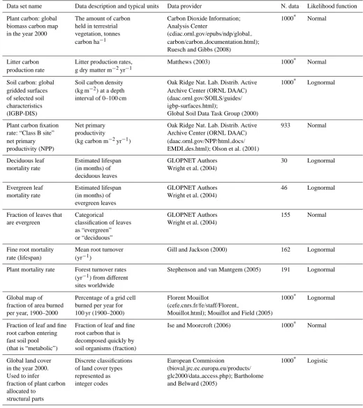
Table 1. Source data on carbon stocks and flows used in our study for model training and evaluation.

Data set name Data description and typical units Data provider N. data Likelihood function

Plant carbon: global The amount of carbon Carbon Dioxide Information; 1000* Normal

biomass carbon map held in terrestrial Analysis Center

in the year 2000 vegetation, tonnes (cdiac.ornl.gov/epubs/ndp/global

carbon ha−1 carbon/carbon documentation.html);

Ruesch and Gibbs (2008)

Litter carbon Litter production rates, Matthews (2003) 1000* Normal

production rate g dry matter m−2yr−1

Soil carbon: global Soil carbon density Oak Ridge Nat. Lab. Distrib. Active 1000* Lognormal

gridded surfaces (kg m−2)at a depth Archive Center (ORNL DAAC)

of selected soil interval of 0–100 cm (daac.ornl.gov/SOILS/guides/

characteristics igbp-surfaces.html);

(IGBP-DIS) Global Soil Data Task Group (2000)

Plant carbon fixation Net primary Oak Ridge Nat. Lab. Distrib. Active 933 Normal

rate: “Class B site” productivity Archive Center (ORNL DAAC)

net primary (kg carbon m−2yr−1) (daac.ornl.gov/NPP/html docs/

productivity (NPP) EMDI des.html); Olson et al. (2001)

Deciduous leaf Estimated lifespan GLOPNET Authors 30 Lognormal

mortality rate (in months) of Wright et al. (2004)

deciduous leaves

Evergreen leaf Estimated lifespan GLOPNET Authors 46 Lognormal

mortality rate (in months) of Wright et al. (2004)

evergreen leaves

Fraction of leaves that Categorical GLOPNET Authors 155 Normal

are evergreen classification of leaves Wright et al. (2004)

as “evergreen” or “deciduous”

Fine root mortality Mean root turnover Gill and Jackson (2000) 162 Lognormal

rate (lifespan) (yr−1)

Plant mortality rate Forest turnover rates Stephenson and van Mantgem (2005) 191 Lognormal

(yr−1) from different sites worldwide

Global map of Percentage of a grid cell Florent Mouillot 1000* Lognormal

fraction of area burned burned per year for (cefe.cnrs.fr/fe/staff/Florent

per year, 1900–2000 100 yr (1900–2000) Mouillot.html); Mouillot and Field (2005)

Fraction of leaf and fine Fraction of leaf and fine Ise and Moorcroft (2006) 1000* Normal

root carbon entering root carbon that is

fast soil pool decomposed quickly by

(that is “metabolic”) soil organisms (fraction)

Global land cover Discrete classifications European Commission 1000* Logistic

in the year 2000. of land cover types (bioval.jrc.ec.europa.eu/products/

Used to infer represented as glc2000/data access.php); Bartholome

fraction of plant carbon integer codes and Belward (2005)

allocated to structural parts

Numbers represent those model parameters specifically needed to predict a particular data set. Some models may have taken the outputs of other models as their inputs, and therefore may implicitly include more model parameters.∗Approximate numbers of data points obtained through random stratified sampling of gridded global data.

Page 45 of 54

15.

Figures

1198

1199

Fig. 1 |

Summary of the inferred climate dependence of the terrestrial carbon cycle within

1200

our terrestrial carbon model. The inferred climate dependence of each component is shown

1201

in red (inferred using the full model and all data sets), grey (inferred using minimal subsets

1202

of the model) and, to illustrate the major structural uncertainty in plant mortality (h), in blue

1203

(inferred using the full model but omitting the plant mortality data). Lines and shading are

1204

average median, 5th and 95th percentiles from 10 training data subsets.

1205

1206

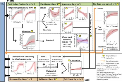
Fig. 1. Summary of the inferred climate dependence of the terrestrial carbon cycle within our terrestrial carbon model. The inferred climate

dependence of each component is shown in red (inferred using the full model and all data sets), grey (inferred using minimal subsets of the model) and, to illustrate the major structural uncertainty in plant mortality (h), in blue (inferred using the full model but omitting the plant mortality data). Lines and shading are average median, 5th and 95th percentiles from 10 training data subsets.

set (over-fitting). Over-fitting can still occur when adopting this approach if model refinement goes through many itera-tions and the same training and evaluation sets are used. We therefore first removed a fraction of each data set to be used as a final step to assess the performance of our models (the “final test data”). This allows us to test our models against data that played absolutely no role in the model refinement process. We constructed a land surface mask by randomly positioning 0.5 degree squares over the terrestrial land sur-face until approximately 25 % of the terrestrial land sursur-face had been covered. Any data that fell under this mask were removed permanently as final test data. We performed 10-fold cross-validation within our model parameter inference experiments on the data remaining after the removal of the final test data.

4.3 Parameter inference

We used a Bayesian approach to infer the probability distri-butions for the model parameters given our empirical data sets. For every model we used flat (or “uninformative”) prior probability distributions for the parameter values. We assume that the probability of observing the data under all possible hypotheses is 1 (the marginal probability). We also made no

attempt in this study to incorporate or infer errors and biases associated with the observational data. This is potentially an important assumption, and accounting for these errors will be enabled in the future for empirical data sets that contain estimates of observational uncertainty

Under these assumptions, estimating the probability distri-butions of the parameters reduces to requiring the estimation of their likelihood, given the observed carbon data and en-vironmental conditions. This required us to specify a likeli-hood function for each model component, which defines the probability of the data, given any combination of parameters. With this function defined, the posterior probability of each parameter could be estimated. Formally, we assume that L(Pred(Model(Pars,Env))|Obs)∝P (Obs|Pred(Model(Pars,Env))),

where bold text denotes a vector. In words, the likelihoodL of the predictions Pred of the parameterised model given the observations, Obs, is proportional to the probabilityP, of the observations given the particular model predictions. The pre-dictions arise from a particular model with parameters Pars and set of environmental conditions Env.

We used the Filzbach set of code libraries to find the posterior distributions for the parameters of a given model, given the observed carbon data (Obs) and environmental

588 M. J. Smith et al.: The climate dependence of the terrestrial carbon cycle

Page 46 of 54 1207

Fig. 2 | Our prototype automated system used for the construction, parameter estimation 1208

and assessment of multi-component models of arbitrary complexity. This automated system 1209

was used to develop and analyze our model. Inputs are multi-component models and 1210

empirical data. Data are partitioned into training, evaluation and final test sets. Input 1211

libraries provide a common interface to connect code with data. Inference routines use 1212

inference libraries to infer parameter probability distributions. Inference libraries implement 1213

approximate Bayesian inference using Markov Chain Monte Carlo methods with the 1214

Metropolis-Hastings algorithm. A data viewer provides a standard interface for inspecting 1215

inputs and results. See Section 5.1. for details on how to download the framework. 1216

1217

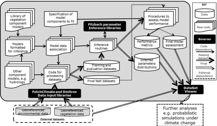
Fig. 2. Our prototype automated system used for the construction, parameter estimation and assessment of multi-component models of

arbitrary complexity. This automated system was used to develop and analyse our model. Inputs are multi-component models and empirical data. Data are partitioned into training, evaluation and final test sets. Input libraries provide a common interface to connect code with data. Inference routines use inference libraries to infer parameter probability distributions. Inference libraries implement approximate Bayesian inference using Markov chain Monte Carlo methods with the Metropolis–Hastings algorithm. A data viewer provides a standard interface for inspecting inputs and results. See Sect. 4.1. for details on how to download the framework.

conditions (Env; http://research.microsoft.com/en-us/um/ cambridge/groups/science/tools/filzbach/filzbach.htm). Filzbach implements Markov chain Monte Carlo sampling of parameter space given a set of parameters to be varied (Pars) and likelihood function (L; Gilks et al., 1996). It uses the Metropolis–Hastings algorithm to accept or reject sets of parameter values when compared to the likelihood associated with the parameter values of the previous iteration of the Markov chain (Gilks et al., 1996). In our study, the likelihood function used by Filzbach may depend on the likelihoods associated with several sub-component models, depending on the model parameter inference experiment being run (outlined below, and see Fig. 3 for details). The specific likelihood function chosen to assess each model component against its corresponding empirical data set is detailed in Table 1.

The data sets used contain different relative frequencies of data for different climate regions of the world. We down-weighted the log-likelihoods assigned to data points in direct proportion to the relative frequency of data in their respective Holdridge life zones (Holdridge, 1967). This avoids biasing the model parameter inference procedures towards parameter values that predict well those regions of the world that are most frequently represented in the data.

4.4 Parameter inference experiments

We investigated the sensitivity of the inferred model func-tional forms and model performance metrics to using dif-ferent combinations of model components and data sets by conducting three different parameter inference experimental protocols described below.

4.4.1 Build-up experiments

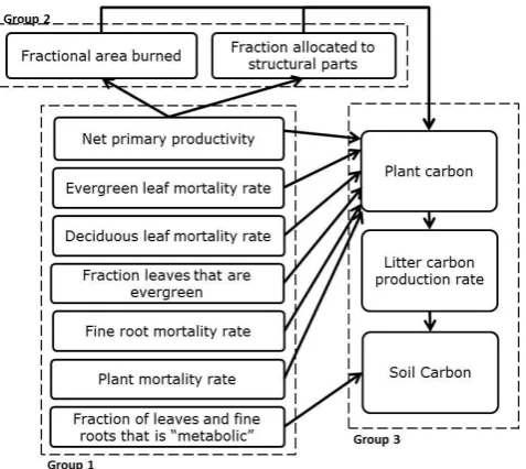
We inferred parameters to each of the component models in-dicated in Fig. 3 alongside those of the models on which they depend to make predictions. We refer to these experiments as “build-up”, because we started by inferring the parameters to the group 1 models individually and then inferred those to the group 2 models (alongside those of the NPP model), be-fore inferring parameters to each of the group 3 models (and those of the sub-components on which they depend), incre-mentally working towards inferring all the parameters in all components of the terrestrial carbon model simultaneously (the 12th experiment).

Page 47 of 54

1218

Fig. 3 | The full terrestrial carbon model can be represented as a factor graph. All boxes 1219

represent model components with accompanying data. Arrows connect a model that acts as 1220

a subcomponent (tail of arrow) to another model (head of arrow). Models within Group 1 1221

do not require predictions from other models to predict their accompanying data sets. 1222

Group 2 models require predictions from the net primary productivity model. Group 3 1223

models require input from several model components. 1224

1225

Fig. 3. The full terrestrial carbon model can be represented as a

fac-tor graph. All boxes represent model components with accompany-ing data. Arrows connect a model that acts as a subcomponent (tail of arrow) to another model (head of arrow). Models within group 1 do not require predictions from other models to predict their ac-companying data sets. Group 2 models require predictions from the net primary productivity model. Group 3 models require input from several model components.

4.4.2 Omit-data experiments

We sequentially omitted an entire data set associated with each model component in Fig. 3 prior to inferring the param-eters of the full model. This enables investigation of how im-portant the information contained in a given data set is for the inferred parameter probability distributions. Each evaluation step also included a fold of the omitted data sets. However, this approach does not allow us to estimate process error as-sociated with a given model in the absence of its asas-sociated empirical data. We therefore used the posterior parameter es-timates of process error obtained from inferring the parame-ters of the full model with all empirical data sets when per-forming model evaluation.

4.4.3 Replace-null experiments

We sequentially replaced a model component in Fig. 3 with a null model consisting of an inferred constant and associated error. This allows us to investigate how important the climate dependency of a particular model is for the predictive per-formance of other components and their inferred parameter values.

4.4.4 Assessing predictive performance

In general, we calculated performance metrics for each sam-ple of parameter values from the Markov chain after the burn-in procedure. The burn-burn-in period was always 20 000 itera-tions, and the Markov chain length used for parameter sam-pling was always 120 000 iterations and was subsampled ev-ery 100 iterations. This enabled us to also take mean, median and 95th percentiles of various performance metrics over the set of sampled parameter values.

5 Results

5.1 Full model

Overall we infer climatically varying functions for all com-ponent processes to our terrestrial carbon cycle model when fitted using all available data sets (red functional relation-ships in Fig. 1). The inferred climate dependencies of net primary productivity (NPP), increasing but saturating func-tions of temperature and precipitation (Fig. 1a, b), are consis-tent with what was established for the classic MIAMI model (Leith, 1975). The proportion of fixed carbon allocated to wood (versus and leaves and fine roots) varies continuously as a sigmoid function of NPP and increases to around 0.35 for the most productive locations (Fig. 1c). The four pro-cesses then determining carbon loss rates have contrasting climate dependencies (Fig. 1d–h). Fire increases with dry season length (combustibility) and NPP (fuel), as expected (Fig. 1i, j; Kloster at al., 2010). Contrasting dependencies of evergreen and deciduous leaf mortality (Fig. 1e, f) are in-ferred, with the relative frequency of evergreen versus decid-uous leaves being U-shaped against annual frost frequency (Fig. 1d). This highlights the relatively complex climate de-pendence of leaf lifespan globally (van Ommen Kloeke et al., 2011). Fine root mortality rate is inferred to increase with mean annual temperature as expected (Fig. 1g; Gill and Jack-son, 2000). A relatively flat relationship for the climate de-pendency of plant mortality is inferred (Fig. 1h); however, this actually results from contradictory information from dif-ferent data sets under our assumed model formulation (de-tails below). We infer no strong climate dependency in the fraction of dead leaves and roots initially allocated between the different soil pools (Fig. 1k). For the soil component, we infer temperature and moisture dependencies of the classical three-pool soil model that are consistent with previous find-ings (Fig. 1l, m; Ise and Moorcroft, 2008).

The lack of a relationship for plant mortality was unex-pected, because a previous study (Stephenson and van Mant-gem, 2005), using the same empirical data on plant mortal-ity rates, identified a positive relationship between mortalmortal-ity rates and productivity – a close correlate of evapotranspira-tion rates (Leith, 1975). Further analysis reveals this incon-sistency to be due to differences in the information implied

590 M. J. Smith et al.: The climate dependence of the terrestrial carbon cycle

Page 48 of 54 1226

Fig. 4|

Performance assessments of the terrestrial carbon model. (A) Pearson’s correlation,

1227

(B) the coefficient of determination or (C) the probability of the model relative to a null

1228

model (Gelfand and Day, 1994). Separate data subsets were used for parameter inference

1229

and model evaluation to avoid over-fitting. A final test data subset was reserved (never used

1230

during model development) to provide an independent estimate of the likely predictive

1231

ability when the model is applied to locations that have not been observed. Assessments

1232

against evaluation and final test data are in grey and red, respectively, with n being the

1233

respective mean or absolute number of data points per assessment. Dots and error bars are

1234

average medians, 5th and 95th percentiles in (A) and (B) and medians, maxima and minima

1235

in (C) using parameter distributions inferred from 10 training data subsets. Insufficient

1236

evaluation data existed to calculate (A) and (B) for the deciduous leaf mortality model.

1237

1238

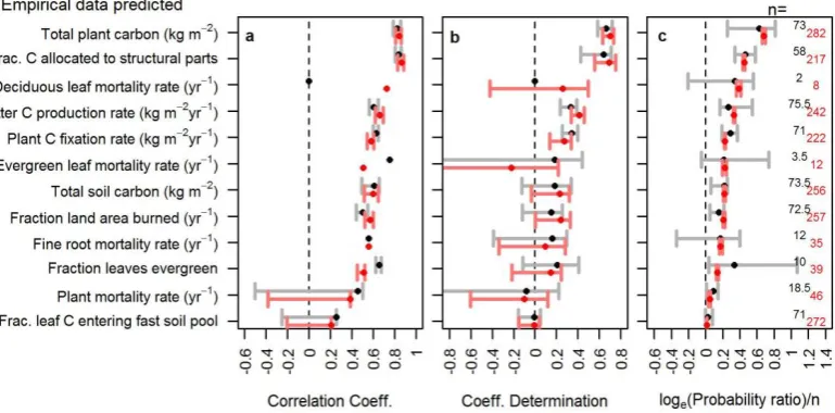
Fig. 4. Performance assessments of the terrestrial carbon model: (a) Pearson’s correlation, (b) the coefficient of determination and (c)

the probability of the model relative to a null model (Gelfand and Day, 1994). Separate data subsets were used for parameter inference and model evaluation to avoid over-fitting. A final test data subset was reserved (never used during model development) to provide an independent estimate of the likely predictive ability when the model is applied to locations that have not been observed. Assessments against evaluation and final test data are in grey and red, respectively, withnbeing the respective mean or absolute number of data points per assessment. Dots and error bars are average medians, 5th and 95th percentiles in (a) and (b) and medians, maxima and minima in (c) using parameter distributions inferred from 10 training data subsets. Insufficient evaluation data existed to calculate (a) and (b) for the deciduous leaf mortality model.

by different empirical data sets under our assumed model for-mulation. We infer qualitatively different climate dependence from the plant mortality data alone (a positive relationship, Fig. 1h (grey), as found by Stephenson and van Mantgem, 2005), from all model components and empirical data sets together (a flat relationship, Fig. 1h (red)), or using all model components but omitting individual data sets (omitting plant mortality data gives a negative relationship, Fig. 1h (blue), omitting the plant carbon data gives a positive relationship, similar to Fig. 1h (grey)). These results indicate a clear dis-crepancy between the information on the climate dependency of plant mortality implied by the mortality data itself and that implied by the other plant carbon data sets under the assumed model formulation. On this basis we identify global plant mortality rates as a major “structural uncertainty” in our terrestrial carbon model.

Other than the non-climatically dependent functions, the climate dependencies inferred for the full terrestrial carbon model tend to make predictions that both are significantly positively correlated with the evaluation data sets (Fig. 4a), and tend to explain a positive fraction of the variation within each data set (Fig. 4b). The plant carbon data set is predicted particularly well (final test data median Pearson’sr=0.84 (5 % and 95 % confidence intervals=0.81, 0.86), coefficient of determination = 0.70 (0.63, 0.77)), as are data on litter pro-duction rate, plant carbon fixation rate and the fraction of carbon allocated to structural plant parts, for all of which the model always explains a positive fraction of the

varia-tion in the data at a 95 % confidence level (Fig. 4b). Com-paring the performance of the full model to one in which the relevant model component is replaced with a null model sup-ports choosing the climate-dependent model for all processes (Fig. 4c) except for the two component processes for which we inferred no climate dependencies.

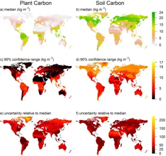
When applied at global scales, the terrestrial carbon model predicts global patterns of equilibrium plant and soil carbon that match the known patterns well (Fig. 5a, b; calculated us-ing the New et al., 2002; and Batjes, 2000 gridded data sets for environmental variables). We estimate that the absolute uncertainty is positively related to the median (Fig. 5c, d) for both carbon pools. For plant carbon, relative uncertainty (absolute uncertainty/median prediction) tends to be higher in areas in which the model predicts vegetation that is in-termediate between being maximally woody and completely non-woody (Fig. 5e), owing to the contrasting mortality rates of these different carbon pools (Fig. 1e–h). Relative uncer-tainty is also higher over Greenland, and we expect this is because of the inflation of uncertainty under extrapolation: the extreme environments in that region are out of the ranges represented in our data (Fig. 5e). We believe a similar phe-nomenon explains the relatively higher uncertainty in predic-tions of soil carbon in extremely dry or cold environments (Fig. 5f).

The inferred climate dependencies in the terrestrial car-bon model, other than the plant mortality function, gener-ally support those that have been found in previous studies,

indicating their consistency when considered as part of the overall system. Although the qualitative nature of many of these dependencies is consistent with previous knowledge, our estimates of parameter values for these functions (and the associated uncertainty in those parameter estimates) are new. Our analysis also highlighted a number of new insights into the performance of these climate-dependent functions as detailed below.

Although the inferred climate dependencies of NPP (Fig. 1a, b) are consistent with the MIAMI model (Leith, 1975), one parameter is not-well constrained by the data: the parameter controlling NPP at zero degrees Celcius (t1in

Eq. C1b) does not converge. Instead, the sigmoid response of NPP to temperature is constrained by the parameter con-trolling the gradient of the temperature dependency,t2. This

implies that the temperature-dependent function may actu-ally be over-complex for our purposes. Further investiga-tions (omitted for brevity) involving removing this param-eter and refitting the model reveal that this and other under-constrained parameters discussed below have little effect on model predictive accuracy. Plots of predictions versus ob-servations also reveal a noisy positive relationship, with the model underestimating NPP for sites with NPP greater than around 1.0 kg m−2yr−1– a property that has been noted pre-viously for the MIAMI model (Fig. 6a; Friedlingstein et al., 1992; Dai and Fung, 1993).

The shape of the function controlling the proportion of fixed carbon allocated to structural components implies that struc-tural tissue only makes up around 10 % of vegetation carbon at NPP values of around 0.5 kg m−2yr−1(Fig. 1c). We expect this probably underestimates structural carbon in vegetation types dominated by low-productive woody vegetation such as some boreal forests (Kicklighter et al., 1999), although we have not verified this.

The wide confidence intervals in the function predicting the fraction of vegetation leaves that are evergreen imply rel-atively high uncertainty, and inspection of the relationship between predictions and observations makes clear why this is the case, with several observations lying far from the 1:1 line (Fig. 6b). Despite this, the correlation between obser-vations and predictions is relatively high (Fig. 4a), probably due to the dominance of sites in the data set that are either entirely evergreen (44 %) or entirely deciduous (14 %). We anticipate that the low quantity of data in the data sets on leaf characteristics (the most sparse data in our collection; Table 1) strongly influences the variation in model predictive performance for those climate dependencies.

Our inference of the climate dependencies of fire fre-quency globally again highlights some redundant model pa-rameters: the scaling constantcfand the two half saturation

constants, lfshalfsat and NPPhalfsat, are poorly constrained.

This implies that the model could be reformulated with fewer parameters and still predict the data with the same accuracy. Although the correlation between predictions and observa-tions is relatively strong for this data set (Fig. 4a, b), visual

inspection of observational data versus predictions implies a lower predictive performance at low fire return intervals (fraction of burned per year) and a tendency to underestimate the fire return interval overall (Fig. 6g).

Although plant carbon is predicted well, the plots of pre-dictions versus observations indicate some notable outliers at low carbon contents, where carbon is predicted to be much higher that observed for some sites (Fig. 6h). These sites ap-pear to be associated with tropical vegetation that has been classified as grasslands and shrublands in the global land cover map and have been assigned low carbon content (data omitted for brevity), in contrast to the predictions of the model.

For the soil model we could, again, not fully constrain all model parameters. The parameter downscaling soil decom-position rates as a function of extremely high temperatures (tscin Eq. C8a) and the parameters controlling the optimum

moisture content for decomposition and downscaling param-eter of decomposition rates in extremely wet conditions (msc

andmthresh, in Eq. C8c) are probably all poorly constrained,

a result of lacking sufficient data representing such extreme environments.

5.2 Build-up experiments

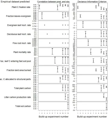
The build-up experiments show that the performance of some model components changes as they become part of larger model structures (Fig. 7). The major result from these exper-iments is the qualitative change in the inferred climate de-pendency of plant mortality upon being connected to the full model, as mentioned above (Fig. 1k). The consequent change in model predictions is clearly seen in the plots of predic-tions versus observed data in which a noisy positive relation-ship between predictions and observations is apparent when the plant mortality model is fitted to the plant mortality data alone, whereas a relatively flat relationship is observed for the model fitted as part of the full model structure (Fig. 6k, l). The net primary productivity model (NPP) improves in predictive performance when it is connected to the full model, showing higher correlation coefficients and an im-proved fit to the training data (lower deviance information criterion values; Fig. 7). Lower uncertainties in NPP func-tional forms are also visible for the full model compared to when the model is fitted to the NPP data alone (grey versus red in Fig. 1a, b). This implies that information from other model components helps to further constrain the climate de-pendence of NPP. The component predicting the fraction of plant material that is woody exhibits a poorer fit to the train-ing data as it is connected to other model components but still slightly increases in predictive performance (Fig. 7). Con-necting this component to plant carbon also enables the pa-rameter controlling the maximum carbon allocation fractions to wood to be inferred (grey versus red in Fig. 1c). Connect-ing the model predictConnect-ing litter production to the full model structure improves its fit to the training data, whereas the

592 M. J. Smith et al.: The climate dependence of the terrestrial carbon cycle

Page

49

of

54

1239

Fig. 5|

Predicted global distributions of equilibrium plant and soil carbon. These match the

1240

known patterns well based on visual inspection. (a, b) Mean median prediction of plant and

1241

soil carbon from parameter distributions inferred from 10 training data subsets. (c, d)

1242

uncertainty range spanned by the 5th and 95th% confidence intervals. (e, f) Uncertainty

1243

relative to the median. Spatial resolution is 10 arc minutes (18.5km at the equator).

1244

1245

Fig. 5. Predicted global distributions of equilibrium plant and soil carbon. These match the known patterns well based on visual inspection. (a), (b) Mean median prediction of plant and soil carbon from parameter distributions inferred from 10 training data subsets. (c), (d)

Uncer-tainty range spanned by the 5th and 95th % confidence intervals. (e), (f) UncerUncer-tainty relative to the median. Spatial resolution is 10 arcmin (18.5 km at the Equator).

opposite is the case for the model predicting fraction of land area burned (Fig. 7). However, none of these effects signif-icantly alter the correlation between predictions and obser-vations in the evaluation data, and they only cause minor re-ductions in the confidence intervals of the functional forms of the fire model (grey versus red in Fig. 1i, j).

5.3 Omit-data experiments

The most notable effects of omitting data sets when infer-ring parameters to the full models were on the parameters of the plant mortality climate dependency, as reported above. Otherwise, omitting individual data sets when fitting the full model does not dramatically influence the performance of the model at predicting the data sets that had not been removed (we omit details for brevity). Constraining the parameters of some components is entirely dependent on the presence of their corresponding data set. This is the case for the fraction of leaves that are evergreen, the mortality rates of evergreen and deciduous leaves, fine root mortality rates and soil de-composition rates and indicates that the prediction of other connected components, such as plant carbon for example, is

not dependent on the predictive accuracy of those compo-nents. In contrast, omitting the data for the NPP model still results in the inference of very similar parameter values, in-dicating a strong dependency on those parameter values for predicting other empirical data sets.

5.4 Replace-null experiments

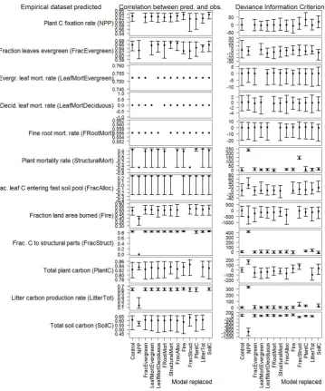
In general, and as expected, replacing a component with a model predicting no climate dependency strongly influences the predictive performance of that component in the cases where evidence exists for a climate dependency (Fig. 8). For some components this results in negligible effects on the pre-dictive performance of the rest of the model. However, for the NPP model, replacement strongly influences the predic-tive performance of other components. This is not surprising, given that it is the initial carbon input term for the plant car-bon pools.

Page

50

of

54

1246

Fig. 6 |

Model predictions versus observed empirical data (omitting the 25% final test data).

1247

Predictions were made using all 10 posterior parameter probability distributions from

10-1248

fold model fitting. Points show the average median prediction and error bars show the

1249

average upper and lower 95% confidence intervals. a)-k) are predictions from the full model

1250

trained to all empirical data sets and l) are predictions from the plant mortality model

1251

trained to the plant mortality data alone.

1252

1253

Fig. 6. Model predictions versus observed empirical data (omitting the 25 % final test data). Predictions were made using all 10 posterior

parameter probability distributions from 10-fold model fitting. Points show the average median prediction, and error bars show the average upper and lower 95 % confidence intervals. (a–k) show predictions from the full model trained to all empirical data sets, and (l) shows predictions from the plant mortality model trained to the plant mortality data alone.

6 Discussion

6.1 The degree of empirical support for the component processes

One of our key aims was to establish a baseline terrestrial car-bon model to support future work in which we had assessed the empirical support for every component process, including clearly characterising and incorporating parameter uncertain-ties. Our new methodology has clearly achieved that, and it also illustrates how the adoption of such a methodology in the future development of terrestrial carbon models could

ac-celerate the identification of where their key inconsistencies lie, both with each other and with empirical data.

We adopted a relatively simple model here, and we hy-pothesise that it is probably too simple and uncertain to pro-vide informative projections of future terrestrial carbon dy-namics. For example, while we adopted the MIAMI model as a convenient and well-recognised, simple model of net primary productivity, it has several well-known limitations (e.g. Bonan, 1993) including being insensitive to changes in atmospheric CO2 concentrations (discussed further

be-low). Rather, what we aimed to do was to develop and im-plement methodology to enable quantitative comparisons of

594 M. J. Smith et al.: The climate dependence of the terrestrial carbon cycle

Page 51 of 54

1254

Fig. 7 |

Correlations between model predictions and hold-out evaluation data (left) and

1255

Deviance Information Criterion (DIC) values (right) obtained from different model fitting

1256

experiments (Gelman et al. 2004). DIC values have been normalised relative to the

lowest-1257

build up experiment number predicting the data set indicated. The presence of confidence

1258

intervals for a given experiment number indicates whether a model component was used in

1259

a model fitting experiment. Points represent the average median estimate using the

1260

parameter probability distributions obtained from 10-fold model fitting and the whiskers

1261

are average 95% confidence intervals.

1262

1263

Fig. 7. Correlations between model predictions and hold-out evaluation data (left) and deviance information criterion (DIC) values (right)

obtained from different model fitting experiments (Gelman et al., 2004). DIC values have been normalised relative to the lowest build-up experiment number predicting the data set indicated. The presence of confidence intervals for a given experiment number indicates whether a model component was used in a model fitting experiment. Points represent the average median estimate using the parameter probability distributions obtained from 10-fold model fitting, and the whiskers are average 95 % confidence intervals.

alternative representations of component processes such as NPP in the future (e.g. those documented in Adams, 2004). Setting out to data-constrain all component processes also forced us to propose new models for some components, such as that for leaf mortality rates based on van Ommen Kloeke et al. (2011). Conducting model development in this way en-ables the empirical evidence for such new component formu-lations to be rapidly assessed and modified if necessary be-fore becoming a longer-term feature of the model. The omit-data experiments also illustrated that the parameters of a new component can be estimated even without any direct data on the process in question, if enough data are included on other connected model components. Subsequently, the direct data,

if they become available, could further reduce uncertainty in the functional form and parameters for the new component.

Skill at predicting the data on the terrestrial carbon cy-cle at equilibrium, as we have shown here, is no guaran-tee that the model can accurately capture the temporal dy-namics of the carbon cycle that other data assimilation stud-ies have focussed on (Scholze et al., 2007; Ricciuto et al., 2011). For example, our model does not account for carbon dioxide fertilisation effects that are likely to have had, and could continue to have, a major influence on vegetation car-bon fixation potential into the future (Friedlingstein et al., 2003). We therefore see a pressing need to build on our rigor-ous approach and begin the process of comparing alternative formulations of component models, model structures, and

different data sets. Such studies would obviously consider alternative representations of canopy photosynthesis (Purves and Pacala, 2008), including not only carbon dioxide fertil-isation effects (Friedlingstein et al., 2003), but also the dy-namics of other resources such as water and nitrogen (Goll et al., 2012), the importance of different plant functional types, vegetation traits, successional processes and permafrost car-bon thawing, to name a few (see Arneth et al., 2012; for a de-tailed discussion). Although we developed our model within a generalized framework so that it can become a foundation upon which future intercomparisons can be conducted (see Sect. 5.1), it will require further improvements to truly en-able detailed intercomparisons of state-of-the-art terrestrial carbon models. Enabling the inference of the parameters of dynamical models using time-varying data, and the quantifi-cation, assessment and propagation of errors in the observa-tional data are two key necessary refinements to enable such studies.

Future studies should also investigate the effects of in-corporating more and improved data sets for data assimila-tion and model testing than we did here. We deliberately se-lected data sets that were relatively easy to obtain, process and share. It is reassuring that these were sufficient to infer most of the known climate dependencies. However, further constraining and testing the more detailed terrestrial carbon models will require new data sets that document temporal dy-namics and, more generally, whichever data have the greatest potential to minimise uncertainty in model predictions. Here we made no use of the valuable FLUXNET (http://fluxnet. ornl.gov/) data sets on water and carbon fluxes nor the FPAR data (http://modis.gsfc.nasa.gov/data/dataprod/dataproducts. php?MOD NUMBER=15). We expect that incorporating such data could assist greatly in constraining and comparing any dynamical models developed in the future. There have already been developments in this direction, especially in constraining terrestrial carbon models with carbon flux data (Knorr and Heimann, 2001; Kaminski et al., 2012; Scholze et al., 2007; Ricciuto et al., 2011). Future developments should build from these studies to enable more detailed process-based models to be data-constrained within our framework, although it will be important to take a balanced approach to refining components and not, for example, focus on refining the representation of photosynthesis if it occurs at the ex-pense of refining other components, such as mortality, which has received much less attention to date.

While we demonstrated here how multiple component processes can be data-constrained using multiple data sets, there is obviously a question about how to assess models when they are projected under future scenarios, for which no observational data can exist. This problem can never be solved fully, and in principle vegetation could exhibit changes, or suffer perturbations, that have never been ob-served, either naturally or under artificial perturbations. Our approach offers the promise of being able to identify model components for which improved understanding would be

most important, by decomposing changes in the output vari-ables of interest (e.g. soil carbon) to changes in different pro-cesses (e.g. the effects of extreme temperatures on soil de-composition rates), and then finding out which data sets are most important for improving those components. Under our framework the results of key experiments, such as manipula-tive experiments, or of other passive observations could then be included as additional data constraints.

6.2 Inferred relationships in relation to current understanding

The climate dependencies inferred here mostly confirm those that have been identified previously. However, the identifica-tion of qualitatively different climate dependencies for plant mortality depending on the model formulation and empirical data used, as well as some other more subtle adjustments to other climate dependencies, highlights the value of the sys-temic approach: it enables us to assess how consistent our model of how the overall system functions is with empirical evidence and identify where discrepancies lie.

At present, we do not understand the reason for the struc-tural uncertainty in the climate dependency of plant mortality rates. As a group, the plant carbon data sets imply that mor-tality rates decrease with actual evapotranspiration under our assumed overall model formulation, whereas the plant mor-tality data imply the opposite. Perhaps the high plant mortal-ity rates observed in highly productive sites are inconsistent with the high carbon values recorded for those sites under the inferred climate dependencies. This could have caused the systematic underestimation of net primary productivity in highly productive sites (Fig 6a), leading to lower than ex-pected predictions for plant carbon, which in turn could cause the inferred plant mortality rates for those sites to be higher than observed. There are however other possibilities, such as issues to do with the quality of the plant mortality data or the other plant carbon data sets, the possibility of plant mortal-ity patterns obeying more complex relationships than repre-sented by our mortality component, or missing processes in the model (such as the separation of structural carbon losses between whole plant mortality and the loss of other structural pars such as branches). These possibilities add to recent calls to increase understanding of the role of plant mortality in the global carbon cycle (Stephenson and van Matgem, 2005; van Mantgem et al., 2009; Allen et al., 2010).

6.3 Building a model for future predictions

We do not know how accurate predictions of temporal dy-namics of the carbon cycle from our terrestrial carbon model might be, because we have done no assessments of our model in predicting carbon dynamics. Nonetheless, we can use it to illustrate the concept of using a data-constrained model to in-spect the relative importance of parameter and structural un-certainty in projections. For example, it could be that, despite

596 M. J. Smith et al.: The climate dependence of the terrestrial carbon cycle

Page 52 of 54 1264

Fig. 8 | Correlations between model predictions and hold-out evaluation data (left) and DIC 1265

values (right) obtained from different replace-null model fitting experiments. The presence 1266

of confidence intervals for a given experiment number indicates whether a model 1267

component was used in a model fitting experiment. Points represent the average median 1268

estimate using the parameter probability distributions obtained from 10-fold model fitting 1269

and the whiskers are average 95% confidence intervals. “Control” indicates the results 1270

Fig. 8. Correlations between model predictions and hold-out evaluation data (left) and DIC values (right) obtained from different replace-null

model fitting experiments. Confidence intervals and points have been removed where the empirical dataset predicted corresponds directly to the model replaced. This is because model performance for that component is typically very poor, making it difficult to visualise the performance of the other components. Points represent the average median estimate using the parameter probability distributions obtained from 10-fold model fitting, and the whiskers are average 95 % confidence intervals. “Control” indicates the results obtained for the full model fitted to all data sets.

the uncertainties identified, the model makes relatively well-constrained projections for some features of the carbon cycle, or it could be that the uncertainties tend to combine to give extremely uncertain dynamics. To illustrate this we set the plant and soil carbon pools across the terrestrial land surface to equilibrium in the year 2000 (as in Fig. 5 but at 0.5 deci-mal degree global resolution), and simulated climate change under pessimistic (A1F1) and optimistic (B1) anthropogenic emissions scenarios using our model to explore the plausi-ble importance of these uncertainties (The IPCC Data

Distri-bution Centre; Lowe, 2005; http://www.mad.zmaw.de/IPCC DDC/html/SRES AR4/index.html; see Appendix D for de-tails). We decided to set the land surface to equilibrium car-bon levels to ensure that any changes in the carcar-bon balance were solely due to climate changes, and the climate scenarios were chosen to create two extremes for comparison.

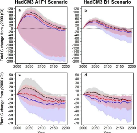
The resulting projected changes in the total terrestrial car-bon balance are similar under both climate forcing scenar-ios, both predicting a net carbon sink up to about 2150 be-fore becoming a carbon source (Fig. 9). However, the time

Page 53 of 54

obtained for the full model fitted to all data sets.

1271

1272

1273

Fig. 9 | Projected changes in terrestrial carbon under two climate change scenarios. These

1274

highlight the potential importance of parameter and structural uncertainty. Lines and

1275

shading represent the average median, 5th and 95th percentile projected changes

1276

(representing parameter uncertainty) from the terrestrial carbon model using parameter

1277

probability distributions inferred from 10 training data subsets. Red, grey and blue

1278

correspond to different climate dependences for plant mortality, representing the major

1279

structural uncertainty in the model (see Fig. 1). Details of how we simulated the model is

1280

given in Appendix C. The additional code necessary to run these simulations is available at

1281

http://research.microsoft.com/en-us/downloads/49ad471e-7411-4f65-910a-1282

2a541f946575/default.aspx and the resulting simulation data is available from

1283

http://download.microsoft.com/download/1/F/D/1FD1F550-69C4-4503-B2FE-1284

B47F94607A7F/MSRTCMSIMData.zip 1285

Fig. 9. Projected changes in terrestrial carbon under two climate

change scenarios. These highlight the potential importance of pa-rameter and structural uncertainty. Lines and shading represent the average median, 5th and 95th percentile projected changes (rep-resenting parameter uncertainty) from the terrestrial carbon model using parameter probability distributions inferred from 10 training data subsets. Red, grey and blue correspond to different climate de-pendences for plant mortality, representing the major structural un-certainty in the model (see Fig. 1). Details of how we simulated the model are given in Appendix C. The additional code necessary to run these simulations is available at research.microsoft.com/en-us/downloads/, and the resulting simulation data are available from download.microsoft.com/download/1/F/D/.

courses of uncertainty in the projections are quite different, with uncertainty higher under the A1F1 scenario and show-ing that the terrestrial carbon cycle could be either a carbon source or a sink over the simulated time period (note that these are not intended as reliable projections). Substituting the alternative models of plant mortality inferred under the different model fitting experiments indicates that this struc-tural uncertainty has only minor quantitative effects on the projected change in the terrestrial carbon balance. Remark-ably, however, this structural uncertainty leads to qualita-tively different predictions for the projected changes in total vegetation carbon up to 2050 (Fig. 9), with positive, rela-tively flat, or negative changes in global vegetation carbon, depending on the mortality model parameterisation chosen. Despite these differences, all simulations predict that vege-tation becomes a net source by 2020. Although these are ex-ploratory simulations, they do emphasise the potential impor-tance and value of considering parameter and structural un-certainties in terrestrial carbon models when attributing con-fidence to projections of the terrestrial carbon cycle in Earth

System Models. Such uncertainty could be decomposed fur-ther into the contributions from different component pro-cesses and even individual parameters and data. We could also begin such simulations with vegetation out of equilib-rium. Such diagnoses are likely to help identify the differ-ent sources of uncertainty in predictions and projections, en-abling the most important sources of uncertainty to be tar-geted for reduction.

Overall, our results complement the progress that has been made in data-constraining terrestrial carbon models (Rayner et al, 2011; Knorr and Heimann, 2001; Scholze et al., 2007; Ricciuto et al., 2011; Zahele et al., 2011) and the devel-opment of frameworks to enable such studies to be per-formed in a repeatable fashion (Scholze et al., 2007; http: //pecanproject.org/). We hope that, by combining these in-sights, the biogeosciences community can rapidly move to-wards identifying the best models for specific purposes, that is, those models which have been shown to be most consis-tent with the available empirical evidence, and which incor-porate uncertainties in model structure and parameter values into their predictions.

Appendix A

Processing of empirical data on carbon stocks and fluxes

We did not actively seek the “best data” pertaining to indi-vidual stocks and fluxes, because we prioritised enabling re-producibility and transparency over obtaining the most accu-rate results. A number of the data sets were only available as gridded land surface data, constructed through analyses of site-based data but for which the original site data were not available (Table 1). For these we generated pseudo-site based data by stratified random sampling. We anticipate that some of our data sets only coarsely represent true carbon stocks or flows at global scales. Moreover, although not all of the data in all data sets represent vegetation in a state of dynam-ical equilibrium, we screened the data sets that incorporate disturbance and anthropogenic effects using the Global Land Cover 2000 vegetation classification map (Bartholome and Belward, 2005) to only select data representative of vegeta-tion at equilibrium.

A1 Vegetation carbon

Global site-based data sets of carbon held in natural ter-restrial vegetation have been compiled previously and used to produce global gridded maps. Unfortunately, the origi-nal source data have not been made generally available. Re-cently, Ruesch and Gibbs (2008) produced a global biomass carbon map for the year 2000 for the entire global land sur-face at 1 km resolution (approximately). This was derived from unique estimates of vegetation carbon values for 124 different carbon zones that were defined by considering the

598 M. J. Smith et al.: The climate dependence of the terrestrial carbon cycle

continent, ecoregion, vegetation type and degree of human disturbance. We used this map to generate pseudo-site based data. We performed stratified random sampling of the Global Land Cover 2000 vegetation classification map (Bartholome and Belward, 2005; which has the same 1 km resolution as the vegetation carbon map) and then for each randomly se-lected point sampled the corresponding vegetation carbon value, conditional on whether the vegetation classification in-dicated specific vegetation types. Specifically, this included classification types 1–9 (generally “tree cover”), excluded type 10 (“tree Cover, burnt”), included types 11–15 (gener-ally shrub or herbaceous cover), and excluded the remaining types 16–22 (not natural or not vegetation).

A2 Litter carbon production

Different studies use terms like “litter production” to mean different aspects of vegetation biomass loss (Matthews, 2003). Here, we define “litter carbon production” as the net mass of carbon lost through natural leaf and fine root mortal-ity (not including fire-induced mortalmortal-ity) per unit area of land surface (m2)per year (yr). This does not include woody lit-ter production through the loss of branches, stems or coarse roots.

Leaf litter production is commonly estimated in the field using litter traps (Matthews, 2003). Studies employing this method rarely estimate root litter production. This led us to consider modelling leaf and fine root litter production sep-arately. However, studies estimating leaf litter production sometimes use it to approximate net primary productivity by assuming that the gains and losses of carbon in the vegetation are balanced (Matthews, 2003). This implies that source data on leaf litter production might not be independent of some of our net primary production data (although we did not check to confirm this). These challenges led us to consider alterna-tive methods for estimating litter carbon production.

Matthews (2003) used multiple methods to estimate litter production. One of these infers litter production from data on soil respiration rates and root respiration rates, by assum-ing that carbon stocks and flows are at equilibrium. Neither of these data sets was used in our model, so we used data generated from this method. A further complication however was that Matthews (2003) never made the source data avail-able. Instead the author presented averages for 30 different vegetation types according to the UNESCO vegetation clas-sification system (Matthews, 1999). We therefore generated pseudo-site based data. To do this we performed stratified random sampling of the UNESCO vegetation classification map (which comes in 1 degree resolution), and for each ran-domly selected point we associated the vegetation type with the litter production value given in column 3D of Table 5 in Matthews (2003). This gives litter dry matter production fig-ures, so we multiplied by 0.5 to approximately convert from dry matter to carbon.

A3 Soil carbon

Global site-based estimates of carbon held in soils under nat-ural terrestrial vegetation have been compiled for decades. We initially considered using the NDP018 data set analysed by Post et al. (1982, 1985) in their studies of global patterns of plant carbon and nitrogen. However, preliminary investi-gations revealed significant differences in the Holdridge cli-mate classifications (Holdridge, 1967) associated with the sites in the NDP018 data and the classifications we ob-tained by using georeferenced climate data from the New et al. (2002) data set. This led us to suspect that the GPS coordinates associated with the NDP018 are not sufficiently accurate to enable a sufficiently accurate estimate of the cli-matic conditions associated with the site. Instead we chose the “Global Gridded Surfaces of Selected Soil Character-istics” (IGBP-DIS) data set produced through the “Global Soil Data Task” project, which was designed specifically to assemble a “reliable and accessible data set on pedosphere properties on a global scale” (Batjes, 2000). We generated pseudo-site based data by performing stratified random sam-pling of the map of soil-carbon density at depth interval of 0–100 cm (which comes in 5 arcmin resolution).

A4 Net primary productivity

Net primary productivity is estimated as the net mass (kg) of carbon fixed by living vegetation per unit area of land sur-face (m2)per year (yr). We selected NPP data compiled for the Ecosystem Model Data Intercomparison project (EMDI, Olson et al., 2001). We selected the Class B “intermediate quality” data set, because it provided a relatively high quan-tity of data (933 unique sites) and represented all of the major vegetation zones of the world.

A5 Mortality rates of deciduous and evergreen leaves, and the fraction of vegetation that is evergreen

We know of no global data sets containing site-based es-timates of leaf turnover rate at the whole vegetation stand level. Data from satellite observations are likely to fill this gap in the future. The lead authors of Wright et al. (2004) provided the GLOPNET database, which, according to Wright et al. (2004), “spans 2548 species from 219 fami-lies at 175 sites” (approximately 1 % of the extant vascular plant species). This database contains georeferenced data for a variety of species-specific leaf traits, for multiple species at a given site, including an estimate of leaf lifespan and whether the leaf is classified as deciduous or evergreen. In a recent analysis of global patterns of leaf mortality, using the GLOPNET database (Wright et al., 2004) supplemented with additional data, van Ommen Kloeke et al. (2011) found clear trends with environmental variables when the decidu-ous and evergreen leaves were treated separately. As a result we calculated the geometric average mortality rate at each