Algorithms for Blind Equalization Based on Relative Gradient and Toeplitz Constraints

(1)

University of Pennsylvania

ScholarlyCommons

Publicly Accessible Penn Dissertations

1-1-2016

Algorithms for Blind Equalization Based on

Relative Gradient and Toeplitz Constraints

Zhengwei Wu

University of Pennsylvania, [email protected]

Follow this and additional works at:http://repository.upenn.edu/edissertations Part of theElectrical and Electronics Commons

This paper is posted at ScholarlyCommons.http://repository.upenn.edu/edissertations/2108 For more information, please [email protected].

Recommended Citation

Wu, Zhengwei, "Algorithms for Blind Equalization Based on Relative Gradient and Toeplitz Constraints" (2016).Publicly Accessible Penn Dissertations. 2108.

(2)

Algorithms for Blind Equalization Based on Relative Gradient and Toeplitz

Constraints

Abstract

Blind Equalization (BE) refers to the problem of recovering the source symbol sequence from a signal received through a channel in the presence of additive noise and channel distortion, when the channel response is unknown and a training sequence is not accessible. To achieve BE, statistical or constellation properties of the source symbols are exploited. In BE algorithms, two main concerns are convergence speed and computational complexity.

In this dissertation, we explore the application of relative gradient for equalizer adaptation with a structure constraint on the equalizer matrix, for fast convergence without excessive computational complexity. We model blind equalization with symbol-rate sampling as a blind source separation (BSS) problem and study two single-carrier transmission schemes, specifically block transmission with guard intervals and continuous transmission. Under either scheme, blind equalization can be achieved using independent component analysis (ICA) algorithms with a Toeplitz or circulant constraint on the structure of the separating matrix. We also develop relative gradient versions of the widely used Bussgang-type algorithms. Processing the equalizer outputs in sliding blocks, we are able to use the relative gradient for adaptation of the Toeplitz constrained equalizer matrix. The use of relative gradient makes the Bussgang condition appear explicitly in the matrix adaptation and speeds up convergence.

For the ICA-based and Bussgang-type algorithms with relative gradient and matrix structure constraints, we simplify the matrix adaptations to obtain equivalent equalizer vector adaptations for reduced computational cost. Efficient implementations with fast Fourier transform, and approximation schemes for the cross-correlation terms used in the adaptation, are shown to further reduce computational cost.

We also consider the use of a relative gradient algorithm for channel shortening in orthogonal frequency division multiplexing (OFDM) systems. The redundancy of the cyclic prefix symbols is used to shorten a channel with a long impulse response. We show interesting preliminary results for a shortening algorithm based on relative gradient.

Degree Type Dissertation

Degree Name

Doctor of Philosophy (PhD)

Graduate Group

Electrical & Systems Engineering

(3)

Keywords

Adaptive filter, Blind equalization, Blind source separation, Independent component analysis, Signal processing

(4)

ALGORITHMS FOR BLIND EQUALIZATION BASED ON RELATIVE GRADIENT AND TOEPLITZ CONSTRAINTS

Zhengwei Wu A DISSERTATION

in

Electrical and Systems Engineering

Presented to the Faculties of the University of Pennsylvania

in

Partial Fulfillment of the Requirements for the Degree of Doctor of Philosophy

2016

Supervisor of Dissertation

_______________________

Saleem A. Kassam, Solomon and Sylvia Charp Professor of Electrical and Systems Engineering

Graduate Group Chairperson

_______________________

Alejandro Ribeiro, Associate Professor of Electrical and Systems Engineering

Dissertation Committee

(5)

ALGORITHMS FOR BLIND EQUALIZATION BASED ON RELATIVE GRADIENT

AND TOEPLITZ CONSTRAINTS

COPYRIGHT

2016 .

(6)

(7)

ACKNOWLEDGEMENT

My deepest gratitude goes to my advisor Prof. Saleem A. Kassam. This dissertation

would not have been possible without his continual guidance, patience and support. During

my studies at Penn, he spent a lot of time guiding me to think independently, to question

critically, and to communicate effectively. I feel incredibly honored to be one of the

students of Prof. Kassam, and extremely lucky to have an advisor who cared so much about

my work and tried so hard to make me a better person. Through the invaluable academic

and life lessons, he has set me an excellent example as a researcher, a mentor and a role

model. I shall remain indebted to his contribution to my rewarding graduate school

experiences, and carry the virtues and principles I learned throughout my life.

I would like to thank the members of my dissertation committee: Prof. Visa Koivunen,

Prof. Santosh S. Venkatesh, and Prof. Saswati Sarkar. I appreciate their time and effort to

review my work and provide valuable comments.

I am grateful for the opportunity to study in the Department of Electrical and Systems

Engineering at Penn. I benefitted greatly from the courses offered and the seminars

organized by the department. My acknowledgement also goes to the technical and

departmental staff for all their help and support.

Completing this dissertation would have been more difficult without the

companionship of my friends at Penn. I am lucky to have met so many excellent and

supportive people, inside and outside the department, who have provided me substantial

(8)

Most importantly, I would like to thank my parents, Jing Xu and Tiemin Wu, for

supporting me, sharing happiness and offering encouragement. They have been a constant

source of unconditional love, strength and patience all these years, without which none of

this would have been possible. I am grateful for their support in my decision to pursue

education abroad, being far away from them. Last but not the least, my appreciation goes

to my beloved husband, Weilu Gao, for his persistent love and compassion. He has always

been there for me, through thick and thin, up and down. I would never be able to have

(9)

ABSTRACT

ALGORITHMS FOR BLIND EQUALIZATION BASED ON RELATIVE

GRADIENT AND TOEPLITZ CONSTRAINTS

Zhengwei Wu

Saleem A. Kassam

Blind Equalization (BE) refers to the problem of recovering the source symbol

sequence from a signal received through a channel in the presence of additive noise and

channel distortion, when the channel response is unknown and a training sequence is not

accessible. To achieve BE, statistical or constellation properties of the source symbols are

exploited. In BE algorithms, two main concerns are convergence speed and computational

complexity.

In this dissertation, we explore the application of relative gradient for equalizer

adaptation with a structure constraint on the equalizer matrix, for fast convergence without

excessive computational complexity. We model blind equalization with symbol-rate

sampling as a blind source separation (BSS) problem and study two single-carrier

transmission schemes, specifically block transmission with guard intervals and continuous

transmission. Under either scheme, blind equalization can be achieved using independent

component analysis (ICA) algorithms with a Toeplitz or circulant constraint on the

structure of the separating matrix. We also develop relative gradient versions of the widely

used Bussgang-type algorithms. Processing the equalizer outputs in sliding blocks, we are

(10)

The use of relative gradient makes the Bussgang condition appear explicitly in the matrix

adaptation and speeds up convergence.

For the ICA-based and Bussgang-type algorithms with relative gradient and matrix

structure constraints, we simplify the matrix adaptations to obtain equivalent equalizer

vector adaptations for reduced computational cost. Efficient implementations with fast

Fourier transform, and approximation schemes for the cross-correlation terms used in the

adaptation, are shown to further reduce computational cost.

We also consider the use of a relative gradient algorithm for channel shortening in

orthogonal frequency division multiplexing (OFDM) systems. The redundancy of the

cyclic prefix symbols is used to shorten a channel with a long impulse response. We show

(11)

Table of Figures

Fig. 2.1 General model of blind equalization. ... 25

Fig. 3.1 Block transmission with cyclic prefix. ... 45

Fig. 3.2 Circulant structure constraint by taking averages. ... 48

Fig. 3.3 Channel impulse response of short minimum phase channel. ... 57

Fig. 3.4 Zero-pole pattern of the minimum phase channel. ... 57

Fig. 3.5 Average ISI of each row of matrix WH_T for the minimum phase system EASI, T-EASI and T-LC-EASI, initialization W (1 0.5 )j I. ... 59

Fig. 3.6 ISI of the rows of matrix WH_C for the minimum phase system with EASI, C-EASI and C-LC-C-EASI, initializationW (1 0.5 )j I. ... 60

Fig. 3.7 Average ISI over multiple minimum phase channels with EASI, EASI and T-LC-EASI. ... 61

Fig. 3.8 Average ISI over multiple minimum phase channels with EASI, EASI and C-LC-EASI. ... 61

Fig. 3.9 ISI of the rows of matrix WH_C for the minimum phase system with EASI, C-EASI and C-LC-C-EASI, initialize center tap of first row of W to value 1 0.5j. 63 Fig. 3.10 Impulse response of the non-minimum phase channel ... 64

Fig. 3.11 Zero-pole pattern of the non-minimum phase channel ... 64

Fig. 3.12 ISI of the rows of matrix WH_C for the non-minimum phase system with EASI, C-EASI and C-LC-EASI, , initialization W (1 0.5 )j I. ... 65

(17)

Fig. 4.2 Structure of the equalizing matrix ... 83

Fig. 4.3 Changing variables from i and j to i j and ... 84

Fig. 4.4 Obtaining the ( )rk , 1 P P 1, from matrix Uk ... 85

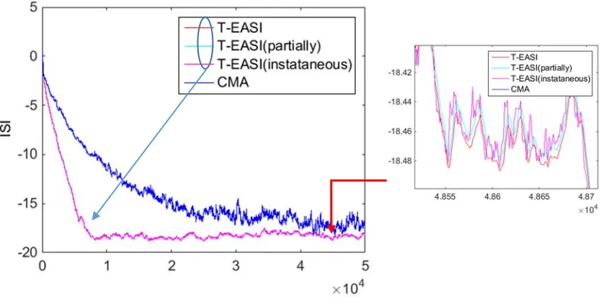
Fig. 4.5 Updating matrix U_k partially with current output ... 93

Fig. 4.6 Channel impulse response of long minimum phase channel ... 97

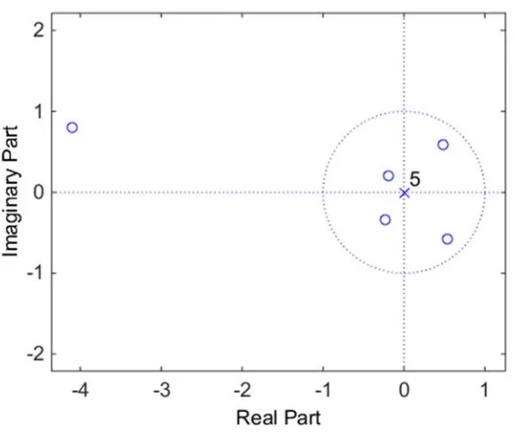
Fig. 4.7 Zero-pole pattern of long minimum phase channel ... 98

Fig. 4.8 ISI of the cascaded system for long minimum phase channel, 64-QAM, SNR=20dB. P 15, M 30_{. ... 98}

Fig. 4.9 Average over 10 runs of the ISI of the cascaded system for long minimum phase channel, 64-QAM, SNR=20dB. P 15, M 30_{. ... 99}

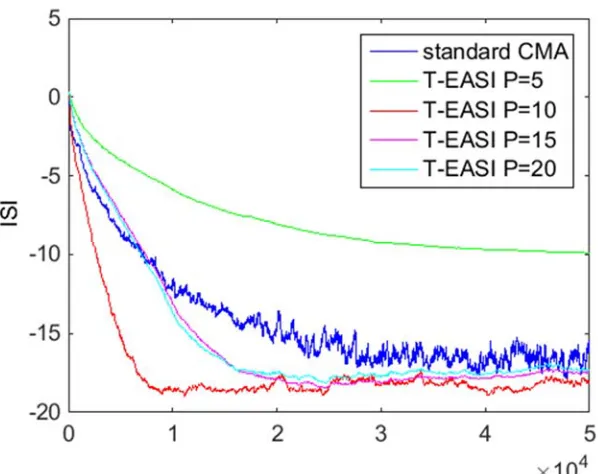
Fig. 4.10 ISI of the cascaded system for long minimum phase channel with different choices of P, 64-QAM, SNR=20dB. M 30_{. ... 99}

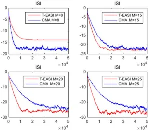
Fig. 4.11 ISI of the cascaded system for long minimum phase channel with different choices of M , P M/ 2, 64-QAM, SNR=20dB. ... 100

Fig. 4.12 Channel impulse response of long non-minimum phase channel ... 100

Fig. 4.13 Zero-pole pattern of long non-minimum phase channel ... 101

Fig. 4.14 ISI of the cascaded system for long non-minimum phase channel, 64-QAM, SNR=20dB. P 10, M 20_{. ... 101}

Fig. 4.15 Average over 10 runs of the ISI of the cascaded system for long non-minimum phase channel, 64-QAM, SNR=20dB. P 10, M 20_{. ... 102}

Fig. 4.16 ISI of the cascaded system for long non-minimum phase channel with different choices of P , 64-QAM, SNR=20dB. M 20_{. ... 102}

(18)

Fig. 4.17 ISI of the cascaded system for long non-minimum phase channel with different

choices of M , P M / 2, 64-QAM, SNR=20dB. ... 103

Fig. 4.18 Channel impulse response of short minimum phase channel ... 104

Fig. 4.19 Zero-pole pattern of short minimum phase channel ... 104

Fig. 4.20 ISI of the cascaded system for short minimum phase channel, 64-QAM,

SNR=20dB. P 10, M 20_{. ... 105}

Fig. 4.21 Average over 10 runs of the ISI of the cascaded system for short minimum

phase channel with different choices of P, 64-QAM, SNR=20dB. M 20_{. ... 105}

Fig. 4.22 ISI of the cascaded system for short minimum phase channel with different

choices of P, 64-QAM, SNR=20dB. M 20_{. ... 106}

Fig. 4.23 ISI of the cascaded system for short minimum phase channel with different

choices of M , P M/ 2, 64-QAM, SNR=20dB. ... 106

Fig. 4.24 Channel impulse response of short non-minimum phase channel ... 107

Fig. 4.25 Zero-pole pattern of short non-minimum phase channel ... 107

Fig. 4.26 ISI of the cascaded system for short non-minimum phase channel, 64-QAM,

SNR=20dB. P 10, M 20_{. ... 108}

Fig. 4.27 Average over 10 runs of the ISI of the cascaded system for short non-minimum

phase channel, 64-QAM, SNR=20dB. P 10, M 20_. ... 108 Fig. 4.28 ISI of the cascaded system for short non-minimum phase channel with different

choices of P, 64-QAM, SNR=20dB. M 20_{. ... 109}

Fig. 4.29 ISI of the cascaded system for short non-minimum phase channel with different

(19)

Fig. 4.30 ISI of the cascaded system for short minimum phase system with

approximation, 64-QAM, SNR=20dB. P 10, M 20_. ... 110 Fig. 4.31 ISI of the cascaded system for long non-minimum phase channel with phase

recovery, 64-QAM, SNR=35dB. P 10, M 20_{. ... 116}

Fig. 4.32 Constellation for recovered symbols, without phase recovery, long

non-minimum phase channel, 64-QAM, SNR=35dB. P 10, M 20_{. ... 116}

Fig. 4.33 Constellation for recovered symbols, with phase recovery, long non-minimum

phase channel, 64-QAM, SNR=35dB. P 10, M 20_{. ... 117}

Fig. 4.34 T-Amari algorithm for long non-minimum phase channel, 64-QAM,

SNR 20dB . P 10, M 20_{. ... 119}

Fig. 4.35 T-Amari algorithm for short minimum phase channel, 64-QAM, SNR 20dB .

10

P , M 20_{. ... 120}

Fig. 4.36 Comparison of T-EASI and T-Amari algorithm for long non-minimum phase

channel, 64-QAM, SNR 20dB . P 10, M 20_{. ... 120}

Fig. 4.37 Comparison of T-EASI and T-Amari algorithm for short minimum phase

channel, 64-QAM, SNR 20dB . P 10,M 20. ... 121

Fig. 5.1 ISI for CMA and block SG CMA. The step-sizes are 3 CMA 1.3 10 ,

3

Block CMA 1.4 10 . SNR 20dB, M 15, P 50. ... 150

Fig. 5.2 ISI for GSA and block SG GSA. The step-sizes are 6 GSA 8 10 ,

6

(20)

Fig. 5.3 ISI for CMA, block SG CMA and VCMA for channel with SNR 20dB ,

16QAM, M 15, P 10. ... 154

Fig. 5.4 Channel impulse response of long non-minimum phase channel. ... 164

Fig. 5.5 ISI for CMA and block RG CMA, i.i.d 64-QAM source. Long non-minimum

phase channel with SNR 20dB , 7

CMA 2 10 ,

7

RG-CMA 6 10 , M 20,

10

P . ... 164

Fig. 5.6 Average over 10 runs of the ISI for CMA and block RG CMA, i.i.d 64-QAM

source. Long non-minimum phase channel ... 165

Fig. 5.7 ISI for CMA and block RG CMA with different choices of P, i.i.d 64-QAM

source. Long non-minimum phase channel with SNR 20dB , M 20. ... 166

Fig. 5.8 ISI for CMA and block RG CMA, correlated 16-QAM source. Long

non-minimum phase channel with SNR 40dB , 6 CMA 3.5 10 ,

6

RG-CMA 13 10 , M 20, P 10. ... 167

Fig. 5.9 ISI for CMA and block CMA with RG with different choices of P, correlated

16-QAM source. Long non-minimum phase channel with SNR 40dB ,

20

M ... 168

Fig. 5.10 ISI for GSA and block RG GSA with different choices of P, i.i.d 64-QAM

source. Long non-minimum phase channel with SNR 20dB, M 20. ... 169

Fig. 5.11 Channel impulse response of short minimum phase channel ... 170

Fig. 5.12 ISI for CMA and block RG CMA with different choices of P, i.i.d 64-QAM

(21)

Fig. 5.13 ISI for GSA and block RG GSA with different choices of P, i.i.d 64-QAM

source. Short minimum phase channel with SNR 20dB, M 20. ... 171

Fig. 5.14 ISI for CMA and block RG CMA with different choices of equalizer order M , for the long non-minimum phase channel. P M / 2. ... 173

Fig. 5.15 ISI for CMA and block RG CMA with different choices of equalizer order M for the short minimum phase channel. P M/ 2. ... 174

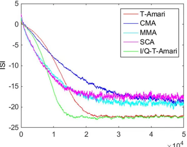
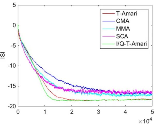
Fig. 5.16 ISI for CMA, block RG CMA and T-EASI with different choices of P, i.i.d 64-QAM source. Long non-minimum phase channel with SNR 20dB, M 20. 177 Fig. 5.17 ISI for CMA, block RG CMA and T-EASI with different choices of P, i.i.d 64-QAM source. Short minimum phase channel with SNR 20dB, M 20. ... 177

Fig. 5.18 ISI for T-EASI, T-Amari, CMA and block RG CMA, correlated 16-QAM source. Long non-minimum phase channel with SNR 40dB , M 20, P 10. ... 180

Fig. 5.19 Norm of equalizer during adaptation. ... 181

Fig. 6.1 OFDM system... 203

Fig. 6.2 Parallel to serial transmission ... 205

Fig. 6.3 ISI of the shortened channel. ... 216

Fig. 6.4 Power ratio of taps inside to those outside the window ... 217

Fig. 6.5 Impulse response of shortened channel, P 10. ... 218

(22)

Chapter 1 Introduction

In digital communication systems, information is represented as symbols that belong to a

finite, discrete constellation. The digital signals are transmitted through an analog channel

between the transmitter and the receiver. Real channels are never ideal, and therefore the

received signal may undergo significant distortion. A widely encountered form of

distortion is caused by non-ideal linear channels, where the frequency response is not flat

in magnitude or not linear in phase across the transmission bandwidth. This results in

inter-symbol interference (ISI). To compensate for this distortion, a linear equalizer can be used

at the receiver. An equalizer can provide significant reduction in ISI.

Traditional equalization is based on transmitted training sequences, and uses the

minimum mean square error criterion for equalizer adaptation [1]. However, it is not

always feasible to send training sequences, which also take up bandwidth for transmission

and reduce the effective data rate. Blind equalization (BE) has the advantage of eliminating

(23)

knowledge of the channel characteristics when no training sequence is used, with the

equalizer converging to a good solution based only on channel outputs during actual data

transmission.

BE has been obtained by exploiting known statistical or constellation properties of the

source symbols [2]–[7]. The BE technique is broadly useful in many applications beyond

classical point–to-point communication channel equalization. The principles of blind

channel equalization can be applied in seismic signal processing [8], in reduction of

microphone-induced ISI in speech recognition [9], [10], and in massive MIMO systems

with time-division duplex (TDD) where the uplink and downlink channels are reciprocal,

allowing BE to be employed by a station based on uplink transmission for better

information about the state of the channel [11]–[14].

There has been extensive work done on blind equalization. Existing algorithms belong

mainly to two types of schemes: one based on known statistical properties of the source

sequence [6], [7], [15], and the other based on the known structure of the signaling

constellation [2]–[4]. The limitations of existing BE algorithms are computational

complexity and/or slow convergence. Especially in practical applications where the

channel is time-varying, fast convergence of channel equalization is necessary [1].

In this dissertation, we modify existing algorithms and develop new ones for BE. We

utilize ideas of relative gradient for equalization adaptation, and constraints on the matrix

structure of the equalizer representation, for faster convergence without excessive

computational cost. First we focus on independent component analysis (ICA)-based

algorithms, where the relative gradient has been used to achieve BSS. Instead of employing

(24)

blind source separation (BSS) problem to be used and the application of an ICA-based

algorithm, we use symbol rate processing. Two transmission schemes are analyzed, where

the symbols are transmitted either in blocks with a guard interval, or continuously without

guard intervals. With either of the schemes, the BE problem can be formulated in matrix

form that has a form similar to that of the BSS problem, except with an additional constraint

on the matrix structure. With a structure-constrained ICA algorithm, independent source

symbols can be recovered with faster convergence. For source symbols with independent

in-phase and quadrature parts, the I/Q independence constraint can be used further for

phase recovery.

We then consider the widely used Bussgang-type algorithms for BE. In the standard

Bussgang-type algorithms, one equalizer output is processed each time with equalizer

adaptations based on standard stochastic gradient descent. In our work, a block processing

scheme for the equalizer outputs is proposed, which allows the use of the relative gradient.

With the relative gradient, the Bussgang condition appears in the adaptation explicitly and

helps speed up convergence.

The block processing approach for both the ICA-based algorithms and the modified

Bussgang-type algorithm shows the interesting connection between these two types of

algorithms. Although the starting points for the two types of algorithms are different, they

end up having related structures. With a matrix structure constraint, the matrix adaptations

for both types of algorithms can be expressed as simpler equalizer vector adaptations.

Approximation schemes simplifying the updates and the use of the fast Fourier transform

(25)

We also propose in a final chapter the use of relative gradient and structure constraint

for channel shortening in orthogonal frequency division multiplexing (OFDM) system.

Channel shortening allows a long channel impulse response to be partially corrected to a

shorter one that can then be equalized based on the OFDM cyclic prefix. The redundancy

due to the cyclic prefix is used in the cost function. We show through simulation the

performance comparison between the proposed and existing algorithms. We also discuss

briefly the potential aspects that may be considered for a more comprehensive evaluation

of the channel shortening algorithms.

1.1 Organization of the Dissertation

There are five main parts in the dissertation: Chapter 2 through Chapter 6.

In Chapter 2, we summarize the fundamental concepts of BSS and BE, including the

notation and the models. The connection between BSS and BE is explained. We introduce

the core idea of ICA, which is a widely used approach for BSS. The “contrast” or criterion

functions and algorithms for ICA methods are explained. Also included in this chapter is a

brief review of BE algorithms, which lays the foundation of further development.

In Chapter 3, we describe two block transmission schemes using guard intervals, for

symbol-rate processing in standard single-carrier systems. With the padded guard intervals

between transmitted blocks, BE can be modeled as a standard BSS problem, which enables

the use of an ICA-based algorithm for BSS. With the guard interval being zeros or a cyclic

prefix, the “separating matrix” has the constraint of being Toeplitz or circulant. We present

(26)

faster convergence compared to standard ICA-based algorithms. I/Q independence

constraint can be combined with the structure constraint for cases where the source symbols

have independent in-phase and quadrature parts. With either the Toeplitz or circulant

constraint, there are repeated elements in the separating matrix. We give an equivalent

computationally efficient adaptation for the vector of elements contained in the separating

matrix.

In Chapter 4, we develop continuous transmission symbol-rate BE schemes related to

the block transmission schemes using ICA-based algorithms. Unlike previous work where

fractional sampling was needed for the use of standard ICA-based algorithms [6], [7], we

show that BE can be achieved with a constrained ICA algorithm using symbol-rate

sampling. We show that the matrix we aim to find for source symbol recovery is a Toeplitz

matrix containing the impulse response of the equalizer. With the Toeplitz constraint

during matrix adaptation, faster convergence can be achieved. The constrained adaptation

leads to an equivalent form of equalizer vector adaptation. Modifications to further reduce

the computational complexity using approximations of vector update equations and the fast

Fourier transform (FFT) is explained in detail in this chapter. Simulation results are shown

for different ICA-based algorithms, and also compared with those of other standard BE

algorithms.

In Chapter 5, we introduce our approach to modifying Bussgang-type algorithms with

relative gradient instead of the standard gradient, using output block processing. By

looking at a block of equalizer outputs, a Toeplitz matrix containing the equalizer vector

can be updated each time based on the cost function from a Bussgang-type algorithm,

(27)

of relative gradient results in an explicit use of the Bussgang condition for faster

convergence. The structure of matrix adaptation with Toeplitz constraint based on

Bussgang-type algorithms is similar to that of the constrained ICA-based algorithms. We

show that these two types of algorithms have a close connection to each other.

In Chapter 6, we investigate briefly the application of relative gradient in channel

shortening algorithms for OFDM systems. In OFDM a cyclic prefix is usually used, which

results in redundancy of the cyclic symbols and the corresponding data symbols in the

OFDM block. When the channel impulse response is shortened to a length smaller than

that of the cyclic prefix, the redundancy between the OFDM symbols and the

corresponding cyclic prefix symbols should be maintained. When multiple cyclic prefix

symbols are taken into consideration, the problem of exploiting redundancy can be

formulated in a matrix expression. This allows the effective use of relative gradient during

adaptation, with the expectation that convergence can be faster. We give preliminary

simulation results and discuss possible directions of future work.

1.2 Contributions and Publications

The main contributions arising from this dissertation are listed below; there are four

conference papers, and two journal papers in preparation for submission.

Zhengwei Wu, Saleem A. Kassam and Kaipeng Li, “Blind Equalization Based On

Blind Separation with Toeplitz Constraint,” Proc. of 48th Asilomar Conference on Signals,

(28)

Zhengwei Wu and Saleem A. Kassam, “Symbol-Rate Blind Equalization Based on

Constrained Blind Separation,” Proc. of 49th Annual Conference on Information Sciences

and Systems (CISS), John Hopkins, MD, 2015.

Zhengwei Wu, Saleem A. Kassam, and Visa Koivunen, “Relative-Gradient

Bussgang-Type Blind Equalization Algorithms,” Proc. of 41st IEEE International Conference on

Acoustic, Speech and Signal Processing (ICASSP), Shanghai, China, 2016.

Zhengwei Wu and Saleem A. Kassam, “Computationally Efficient

Toeplitz-Constrained Blind Equalization Based on Independence,” Proc. of 50th Annual Conference

on Information Sciences and Systems (CISS), Princeton, NJ, 2016.

Zhengwei Wu and Saleem A. Kassam, “ICA-Based Blind Equalization Algorithms

with Toeplitz Constraint,” (In progress).

Zhengwei Wu and Saleem A. Kassam, “Relative-Gradient Bussgang-Type Blind

Equalization Algorithms,” (In progress).

References

(29)

[2] Y. Sato, “A Method of Self-Recovering Equalization for Multilevel Amplitude-Modulation Systems,” IEEE Trans. Commun., vol. 23, no. 6, pp. 679–682, 1975.

[3] D. N. Godard, “Self-Recovering Equalization and Carrier Tracking in Two-Dimensional Data Communication Systems,” IEEE Trans. Commun., vol. 28, no. 11, pp. 1867–1875, 1980.

[4] J. Treichler and B. G. Agee, “A new approach to multipath correction of constant modulus signals,” IEEE Trans. Acoust., vol. 31, no. 2, pp. 459–472, 1983.

[5] O. Shalvi and E. Weinstein, “New criteria for blind deconvolution of nonminimum phase systems (channels),” IEEE Trans. Inf. Theory, vol. 36, no. 2, pp. 312–321, 1990.

[6] H. H. Yang, “On-line blind equalization via on-line blind separation,” Signal Processing, vol. 68, no. 3, pp. 271–281, 1998.

[7] Y. Zhang and S. A. Kassam, “Blind separation and equalization using fractional sampling of digital communications signals,” Signal Processing, vol. 81, no. 12, pp. 2591–2608, 2001.

[8] Y. Li, C. Guo, and T. Fei, “Application of Improved Classical Blind Equalization Algorithm in Seismic Signal Processing,” in Advances in Electric and Electronics, Springer, 2012, pp. 591–598.

[9] L. Mauuary, “Blind equalization in the cepstral domain for robust telephone based speech recognition,” in Signal Processing Conference (EUSIPCO 1998), 9th European, 1998, pp. 1–4.

[10] D. Wang, H. Leung, K.-C. Kwak, and H. Yoon, “Enhanced Speech Recognition with Blind Equalization For Robot‘ WEVER-R2,’” in Robot and Human interactive Communication, 2007. RO-MAN 2007. The 16th IEEE International Symposium on, 2007, pp. 684–688.

[11] D. Neumann, M. Joham, and W. Utschick, “Channel Estimation in Massive MIMO Systems,” arXiv Prepr. arXiv1503.08691, 2015.

[12] J. Jose, A. Ashikhmin, P. Whiting, and S. Vishwanath, “Channel estimation and linear precoding in multiuser multiple-antenna TDD systems,” IEEE Trans. Veh. Technol., vol. 60, no. 5, pp. 2102–2116, 2011.

(30)

[14] H. Q. Ngo and E. G. Larsson, “Blind Estimation of Effective Downlink Channel Gains in Massive MIMO,” 2015.

(31)

Chapter 2 Review of Blind Source Separation

and Blind Equalization

2.1 Introduction

Blind adaptive equalization has been of long-standing interest, and Bussgang-type algorithms for blind equalization (BE) based on gradient descent schemes are well-known.

Blind source separation (BSS) and blind equalization problems have similar goals, recovery of the original signals from their observed mixtures based on limited knowledge of the sources. As a result, BE algorithms based on BSS have also been of interest.

(32)

natural and relative gradient. In this background chapter, we summarize the basic concepts and approaches of BE and BSS.

In Section 2.2, the model of BSS and the well-known Independent Component Analysis (ICA) based algorithms are introduced first. Different criteria that may be used for BSS are given. We summarize the two useful steps in ICA-based approaches: whitening and orthogonalization. A brief discussion of gradient descent based on natural and relative gradient concepts is also given. Since the focus of the dissertation is to obtain better BE schemes, we also introduce the general model of the BE problem in Section 2.3. The relation of the BE model to the BSS problem is explained. Examples of BE algorithms that are widely used are briefly reviewed. Further details related to specific algorithms will be included as we use them in later chapters.

2.2 Review of BSS and ICA

2.2.1 Basic Model

Blind source separation (BSS) is the problem of recovering independent sources from observed mixtures when no information about the mixing process and no training sequence is available. Generally, in BSS problem, there are n independent source signals at time k,

i.e. [ k(1), (2),..., (k k )]

T

k s s s n

s . These sources get mixed, and result in m linear

combinations with unknown coefficients. Expressing this process in matrix form, we have

k k

(33)

where [ _k(1), (2),..., (_k _k )]T

k x x x m

x is the m 1 vector of observations, and A is the

m n matrix of mixture coefficients. It is generally assumed that m n, i.e. there are at least as many observations as sources.

The goal of BSS is to find an n m separating matrix B such that

k k

y Bx (2.2)

contains estimates of the source components ( )s i_k , i 1, 2,...,n. Ideally, the separating matrix should satisfy

BA P, (2.3)

where is a non-singular diagonal matrix, and P is a permutation matrix. In other words, the sources may be recovered to within a scaling and permutation. Perfect recovery means

that BA I, i.e. B is the inverse of A.

One widely applied approach to BSS is that of independent component analysis (ICA) [1]. The basic idea of ICA is that if no more than one source is Gaussian, the signals can be estimated with the simple constraint that recovered signals be statistically independent [1], [2]. The conditions of identifiability, separability, and uniqueness of linear ICA models are studied in [3].

2.2.2 Contrast Functions

In the ICA approach, BSS is usually obtained by defining and optimizing a real-valued

(34)

has the form L( )B E G[ ( )]y . The contrast functions should be designed in a way such that when the sources are separated the optimal value of the contrast function is achieved [4]. There are several different statistical criteria that can be used to define contrast functions, and it has been shown that some of them are closely related. In this part, different examples of the criteria used in ICA methods are reviewed briefly.

Likelihood function

Assume that the sources have joint density function ( 1

)

( ) s ( ( ))

n i i

fs s f s i . By virtue of (2.1), if A is a non-singular matrix, the joint density function of the observation can be expressed as

1 1

( ) | det | ( )

fx x A fs A x . (2.4)

If the joint density function of the sources is known a priori, our goal is then to find a

matrix _{B A} 1_{such that (2.4) is maximized. In other words, we want to get the}

maximum-likelihood estimate of _A 1_.

Using the logarithm of the likelihood function in (2.4), one can define the contrast function based on maximum likelihood as

) 1

(

( ) [ log ( ( )) ] log | det |

M

i

L i

n

s

L B E f y i B . (2.5)

(35)

The maximum likelihood contrast can be shown to be closely related to a group of contrast functions, such as the one based on mutual information of the separated symbols [5], and also the one based on cumulants [4]. These contrast functions are reviewed next.

Mutual information

The mutual information contrast is an information-theoretic measure of dependence between random variables. It is always nonnegative, and is zero when the variables are statistically independent of each other. As a result, the mutual information of the separated components can be used in the contrast function to achieve source separation [5], [6].

Mutual information can be interpreted using entropy or Kullback-Leibler divergence [7]. From either starting point, it can be shown that the mutual information for components in y can be defined as

1

(1)) ( )) (1),..., ( ... (

( (1),..., ( )) [log ] ( ( )) ( ) ( ( ))

n

i

y y n

f f

I y y n E

y H y i H

f y n y , (2.6)

where the sub-index s i( ) of the density function is omitted, and

( ( )) [log ( ( )) ]

H y i E f y i is the entropy. From (2.2) it follows that

( ) ( ) log | det |

H y H x B . (2.7)

Since H( )x is a constant, minimizing (2.6) leads to the contrast function

1

( ) ( ( )) log | det |

[log ( ( )) ] log | det |

n i M i I n

L H y i

E f y i

B B

B

(36)

Comparing (2.8) and (2.5), we see that the two contrast functions differ only by a negative sign. As a result, minimization of the mutual information of the separated symbols is the same as maximization of the likelihood of the observations.

Non-Gaussianity

In addition to the criteria mentioned above, non-Gaussianity can also be used in the definition of contrast functions. According to the central limit theorem, when sources are linearly combined, the distribution of the mixed signal is closer to Gaussian than that of individual non-Gaussian sources [7]. The idea to maximize output non-Gaussianity is therefore to go in the opposite direction of mixing, i.e. to separate the signals.

From information theory we know that among random variables of equal variance, a Gaussian variable has the largest entropy. A measure that is zero for Gaussian variables and gets more positive for variables that are less Gaussian is negentropy. The contrast function based on negentropy can be expressed as

1

( ) ( ( )) ( ( ))

NE Ga s

n

us i

L B H y i H y i , (2.9)

where y_Gauss( )i is a scalar Gaussian random variable that has the same mean and variance

as y i( ), and H y i( ( )) is the entropy of y i( ) [1].

When the separated symbol vector y is preprocessed to be uncorrelated, i.e. [ H]

E yy I, we have

(37)

This implies detB should be a constant since det _E[_xxH] _{does not depend on}_B_{. If we}

look at the mutual information based contrast function (2.8), we can see that it can be written equivalently as

( ) ( ( )) ( ( )) log | det | ( ( )) constant ( )

MI Gauss Gauss

NE

i i i

L H y i H y i H y i

L

B B

B

(2.11)

As a result, when the separated symbols are constrained to be uncorrelated, minimizing mutual information of the estimated components is equivalent to maximizing the sum of their negentropies

Cumulants

The contrast functions mentioned above are based on at least an approximation of the source density function. Now we discuss an approach using high-order statistics that does not depend on the source density. For simplicity, source symbols are assumed to be real in this brief discussion..

Cumulants are high-order statistics that can be used to define contrast functions. For BSS, the most commonly used cumulants are the 2nd_{- and 4}th_{- order ones, which can be}

defined as

( ) [ ( ) ( )]

ij

Cum s E s i s j , (2.12) ( ) [ ( ) ( ) ( ) ( )] [ ( ) ( )] [ ( ) ( )]

[ ( ) ( )] [ ( ) ( )] [ ( ) ( )] [ ( ) ( )].

ijkl

Cum E s i s j s k s l E s i s j E s k s l E s i s k E s j s l E s i s l E s j s k

s

(2.13)

Specially, the 2nd_{-order cumulant terms in (2.12) compose the covariance matrix of vector}

(38)

When the sources in s are independent, the cross-correlation terms in (2.12) and (2.13) vanish, and we have that

2

( )

ij i ij

Cum s , (2.14)

( )

ijkl i ijkl

Cum s , (2.15)

where _ij or _ijkl equals one when all the sub-indices are the same and zero otherwise; and

2

i and i are the variance and kurtosis of source si, i.e.

2 _{[ ( ) ]}2

i E s i , (2.16)

4 2 2

[ ( ) ] 3 [ ( ) ]

i E s i E s i . (2.17)

Cardoso pointed out in [4] that the following function can be shown to be a contrast function:

2

4( ( )

( ) ) ij cumu

ijkl

kl i ijkl

L B y Cum y . (2.18)

At the same time, this function can be interpreted as the quadratic mismatch of the cumulants.

The cumulants-based contrast function is closely related to the maximum likelihood function. When the s and y are symmetrically distributed with distribution that is close to

normal, then using the Edgeworth expansion [8], the maximum likelihood based contrast function can be shown to be related to the following function with the 2nd_{- and 4}th_{- order}

cumulants [4]:

2 4

1 ( ) 12

48 ( ) ( )

ML Appro

L B y y (2.19)

(39)

2 2

2

( ) ij( ) i j j

i i

Cum y

y . (2.20)

Specially, when the outputs are constrained to be of zero mean and unit variance,

[ ( )] 0

E y i and _{E y i}_{[ ( ) ] 1}2 _{, the term}

2( )y defined in (2.20) becomes zero. Under the whitening constraint ₂( ) 0y , it can be shown that 4( )y in (2.18) is equal to

4 4 ( ) 2 i iiii( ) [ 2 ( ( ) 3)]

i

i i

Cum E y i

y y . (2.21)

When the kurtoses of all the sources are negative, then (2.21) becomes the very simple and commonly used kurtosis-maximization contrast function used in [9], [10], [11]:

4

( ) [ ( ) ]

KM

i

L B E y i . (2.22)

We will see in Chapter 3 and 4 that this contrast function leads to a simple nonlinearity that can be used in ICA- based algorithms which can be interpreted as being based on non-linear decorrelation for independence.

2.2.3 Gradient and Online Algorithms

With a specific contrast function L( )B E G[ ( )]y chosen for minimization, the classical approach for obtaining the minimum is steepest descent or gradient descent. In the gradient descent method, we start from an initial positon, and minimize the function iteratively by computing a gradient of the function at the current position and moving in the negative direction of the gradient by a certain amount [7]. The process is repeated until convergence.

(40)

included in Section 5.3. The gradients for complex cases will also be derived and used in Chapter 5.

Relative Gradient and Natural Gradient

A widely-used gradient is the standard gradient, which is usually assumed at the mention of “gradient”. For a contrast function L( )B of matrix B, the standard gradient of the function with respect to the variable B can be expressed as

( ) )

( L

L

B

B B

B . (2.23)

It will be seen from detailed analysis to be given in Chapter 5 and its appendix that when

the contrast function has the expression L( )B E G[ ( )]y , the standard gradient can be derived as

) [ ( ( _E ) ]T

L

B B g y x , (2.24)

where g is the component-wise derivative of function G at y. With the standard gradient, the iterations for minimization are

1 ( )

k k BL

B B B , (2.25)

where is the step-size.

Another gradient that can be used is the relative gradient. For a contrast function L( )B , a perturbation B proportional to the current value of B is considered, where is a matrix with small entries [10]. Writing out the Taylor expansion for ( )L B , we find

( ) ( ) trace[( ( ) T T) ] ( )

L B B L B _BL B B o . (2.26)

(41)

( )R _L₍ ₎ _L₍ ₎ T _E_{[ (} _{) ]}T

B B B B B g y y . (2.27)

The relation between the relative gradient and the standard gradient can be seen from the

expressions (2.24) and (2.27). With relative gradient, the adaptation for matrix B becomes ( )

1 ( )

R

k k B L k k

B B B B . (2.28)

The concept of natural gradient was developed by Amari [6] and used for various problems including the BSS [12]. The starting points of natural gradient and the relative

gradient are different. However, for the BSS problem where the variable B is a non-singular matrix, the two yield the same expression for gradient, and as a result the same adaptation. More details about the relative gradient and natural gradient will be given in Chapter 5.

Online Algorithms

In (2.25) and (2.28), the adaptation for matrix B with standard gradient and relative gradient have been given respectively. Although the contrast function includes expectation, which needs an estimate to be computed, in simple gradient descent methods the expectation is dropped and replaced by its instantaneous value. As a result, the gradient descent method is usually used as stochastic gradient descent.

With the relative gradient, or natural gradient, and dropping the expectation, the adaptation in (2.28) becomes

1 ( )

T

k k k k k

B B g y y B . (2.29)

(42)

1

[ ]

( ) ( )

k k k k

k k

B B B

U y I

y B U

, (2.30)

where ( ) ( ) T

k k k

U y g y y . Online algorithms that have the form of (2.30) can be called

“serial updating”. The advantage of such an algorithm is the property of “equivariance”. If we multiply both sides of (2.30) from the right by the mixing matrix A , we have

1 [ ( )]

k U k k k

C I C s C , (2.31)

where Ck BkA.

In (2.31), the adaptation is characterized by the global system C_k and the source

symbols. For two mixing matrices A and A' with the same sources, if we initialize the separating matrix to be B0 and B0', as long as B A B A0 0' ', the trajectory of the global

system C will be identical. In this case, we say that the adaptive algorithm is equivariant, and offers uniform performance. The equivariance property enables one to deal with BSS problems with an ill-conditioned mixing matrix, and consider the global system as a whole.

2.2.4 Whitening and Orthogonalization

Whitening

In BSS, to make it easier to separate the sources, the observed data is often preprocessed to have uncorrelated components. Mathematically, a zero-mean random vector z is said to be white if its elements are uncorrelated with each other and have unit variance. In other words, for z that is white

[ H]

(43)

Whitening can be obtained through eigenvalue decomposition (EVD). Suppose we want to whiten the mixed signals x with a linear matrix V, and it is transformed to be

z Vx. When z is white, we have

[ H] [ H] H

Ezz V xx VE I. (2.33)

Let _E[ H] xx

C xx be the covariance matrix of x, then by EVD the matrix C_xx can be written as

H

xx

C EDE , (2.34)

where E is the matrix whose columns are the eigenvectors of the covariance matrix C_xx, and D is the diagonal matrix of the eigenvalues of C_xx. As a result, a linear operation with matrix _{V D E}1/2 H_{will make}_{z Vx}_{become white. In fact, whitening matrix is not}

unique, since we can pre-multiply V with an orthogonal matrix and still keep the covariance matrix of z identity.

In addition to algebraic methods such as EVD, whitening can also be performed with on-line algorithms. As stated in [10], the Kullback-Leibler divergence between two normal

distributions with covariances R_z and I can be expressed as

1

( ) Trace( ) log det( )

2 z z

K z R R n (2.35)

where n is the size of vector z. We see that K( ) 0z with equality if and only if R_z I. With the cost function L( )V K( )z K(Vx) and using relative gradient [7], [10], whitening can be performed iteratively with

1 [ ]

H k k z zk k k

(44)

As has been seen in Section 2.2.2 some contrast functions are defined based on the assumption that the mixed signals are white. In such cases, it is important to pre-process the observations so that they are whitened.

Orthogonalization

With whitening as a pre-processing step, the BSS problem reduces to finding an

orthogonal matrix Q such that Qz s, i.e. the separating matrix is B QV . The

orthogonality is based on the pre-whitening step, and is said to operate under the whiteness constraint [13].

With a particular contrast function, the gradient descent method for updating an orthogonal Q will not necessarily make it remain orthogonal automatically. As a result, it

may be beneficial to orthogonalize the matrix at the end of each iteration.

Orthogonalization can be accomplished in many ways [7], and one method uses the following procedure:

1/2 ( H )

Q Q Q Q . (2.37)

It can be shown that the operation in (2.37) is the orthogonal projection of matrix Q onto

the set of orthogonal matrices [14]. The drawback of the method of (2.37) is that a matrix inverse is involved at each iteration. A simpler approach is the following two-step iterative updating:

/ || ||

3 1

2 2

H

Q Q Q

Q Q QQ Q , (2.38)

(45)

The orthogonality and the whitening constraint can also be combined during adaptation. In [10], Cardoso proposed the equivariant adaptive separation via independence (EASI) algorithm which combines the whitening constraint and preserves orthogonality in one step. In the EASI algorithm, the adaptation for the separation matrix is

1 ( ) ( )

H H

k k k k k k k k

H k

B B y y I g y y y g y B , (2.39)

where the vector g y( )_k is the component-wise derivative of the function G( )y in the

contrast function at y_k B x_{k k}. In the updating scheme (2.39), the first two terms in brackets

effect a whitening constraint. The last two terms are to make the relative change skew symmetric so that the orthogonality is obtained with the whitening constraint. The G( )y

function is based on criteria such as those introduced in Section 2.2.2, however it can more

generally be taken to be some reasonable nonlinear function. The term ( ) H k k

g y y can be

interpreted as forcing nonlinear decorrelation for independence of the separated symbols.

2.3 Review of Blind Equalization

2.3.1 Model of Blind Equalization

(46)

Fig. 2.1 General model of blind equalization.

For symbol-rate sampling, the output of the channel at time k can be expressed as

0

( ) L ( ) ( ) ( )

l

x k h l s k l v k , (2.40)

where _h [ (0), (1),..., ( )]_h _h _{h L} T_{is the channel response, and}

{ ( )}v k is an additive white Gaussian noise sequence. The input source sequence is generally assumed to be i.i.d, but some BE algorithms work when the source symbols are correlated.

In BE, suppose an M- th order equalizer with impulse response [ (0), (1),..., ( )]_w _w _{w M} T

w is to be designed, such that the output of the equalizer is

0

( ) M ( ) ( ) T m

k

y k w m x k m w x , (2.41)

where [ ( ), ( 1),..., ( 1)]T k x k x k x k M

x is a length - (M 1) vector containing the

current and past M channel outputs.

Ideally, y k( ) is an approximation of the input symbol with some delay d and possibly a phase shift . In other words, when the impulse response of the channel-equalizer cascaded system is approximately

zeros

(0,...,0,1,0...0)

d ideal _ej

(47)

we consider w to be an ideal equalizer. With an ideal equalizer, the source symbols can be recovered up to a fixed delay and phase shift.

In most adaptive BE algorithms, a single equalizer output is processed each time. To achieve BE, a cost function J(w) E[G(y(k))] that is based on the fit of equalizer outputs to some known signaling constellation property of the source constellation may be defined and optimized.

Suppose the channel outputs are processed in blocks of size P M (P 0) at symbol rate, by sliding along the sequence of channel outputs, with one-symbol shift each time.

Let [ ( ), ( 1),..., ( 1)]T k x k x k x k P M

x be the k-th output block from the channel at

time k, which is influenced by the length- (P M L) source vector

[ ( ), ( 1),..., ( 1)]T k s k s k s k P M L

s . The channel is assumed to be almost

stationary over this observation period. The channel output block of length P M can be expressed in matrix form as

k k k

x Hs v , (2.43)

where [ ( ), ( 1),..., ( 1)]T k v k v k v k P M L

v is the additive noise vector, and H is a

(

) )

(P M P M L _{Toeplitz matrix containing the channel response:}

(0) (1) ( ) 0 (0) (1) ( ) 0

h h h L

H

(0) (1) h h ( )h L

. (2.44)

(48)

in (2.43) has a form similar to the BSS model of (2.1) (ignoring the noise term), and this provides another point of view for the BE problem. Note that the H matrix in (2.43) is an underdetermined matrix with more columns than rows. Although the dimension of H does not satisfy the requirement of a standard BSS problem, it will be seen in later chapters that with some constraints the BE can nonetheless be obtained with ICA-based algorithms.

2.3.2 Blind Equalization Algorithms

Many well-known algorithms for BE use steepest stochastic gradient descent methods for adaptive updates. With a defined cost function J(w) E[G(y(k))] based on some source constellation property, the equalizer coefficients are updated generally according to

*

* 1

( ( ) ( )

, ) _k

k

k k

g y k J

w w

x

w w

w (2.45)

where _w*J( )w is the standard gradient of the cost function J( )w with respect to the conjugate of the equalizer vector for complex case, and g y k( ( )) is the derivative of

( ( ))

G y k with respect to the conjugate of the equalizer output y(k). The details of obtaining gradient when the variable is complex will be shown in the appendix in Chapter 5. In the steady state, if the coefficients of the equalizer converge, we have approximately

*

1 ( ) 0

k k w J

w w w . (2.46)

Following (2.46), it can be shown that for any integer m, the equation

* [ ( ( )) ( ) ] 0

(49)

holds at the steady state, for any integer m . This condition (2.47) is called the Bussgang condition, and an algorithm that has the adaptation of the form (2.45) is called a Bussgang-type algorithm.

Next we will give several examples of the widely used Bussgang-type algorithms, with their cost functions and adaptive update equations. More details about these adaptive BE algorithms will be explained in Chapter 5.

Sato algorithm

The pioneer BE algorithm was the Sato algorithm for PAM signal [15], whose cost function is

Sato Sato

2

( ) [( ( ) sgn( ( ))) ]

J w E y k R y k ,

where _Sato [| ( ) | ]2

[| ( ) |]

E s k R

E s k . The adaptation for the Sato algorithm is

Sat

1 k ( ) osgn( ( )) k

k y k R y k

w w x .

Generalized Sato algorithm

A generalization of the Sato algorithm to complex signals is the generalized Sato algorithm (GSA) [16], with cost function

2 GSA( ) [| ( ) GSAcsgn( ( )) | ]

J w E y k R y k ,

where csgn( ( )) sgn( ( ))y k y k_R jsgn( ( ))y k_I for complex valued number

( ) _R( ) _I( )

y k y k jy k , and _GSA [| ( ) | ]2 [| ( ) | ]2

[| ( ) |] [| ( ) |]

R I

E s k E s k R

E s k E s k . The adaptation is

1 GSA

*

csgn( ( ) ( ))

k k y k R y k k

w w x .

(50)

The Godard algorithm [17] has the cost function defined as

Godar

2 d( ) [(| ( ) | ) ]

p p

J w E y k R ,

where 2 [| ( ) | ] [| ( ) | ] p p p

E s k R

E s k . The adaptation for the Godard algorithm is

2 1

*

(| ( ) | ) ( ) | ( ) | _k

k

p p

k y k Rp y k y k

w w x .

A special case of the Godard algorithm for p 2 is the constant modulus algorithm (CMA) proposed in [18], with the cost function

2 2

CMA( ) [(| ( ) | CMA) ]

J w E y k R .

The adaptation for the CMA is

2

1 CMA

*

(| ( ) | ) ( )

k wk y k R y k xk

w .

Multimodulus algorithm

The multimodulus algorithm (MMA) was proposed in [19] that provides more flexibility than the CMA. The MMA has cost function

2 2

MMA( ) [(| ( ) | MMA) (| ( ) | MMA) ]

p p p p

I R

E y k R k R

J w y ,

where

2 2

MMA

[| ( ) | ] [| ( ) | ] [| ( ) |] [| ( ) |]

p R I

R I

p p

E s k E s k

R

E s k E s k . The adaptation for the MMA has the expression

1 MMA

*

( ) ( )

k k

k e k y k

w w x ,

where

MMA( )k R( ) I( ) e e k je k ,

2 MMA

( ) (| ( ) |p p ) ( ) | ( ) |p R k y kR R y k y kR R

e ,

2 MMA

( ) (| ( ) |p p ) ( ) | ( ) |p I k y kI R y k y kI I

(51)

Square contour algorithm

The square contour algorithm (SCA) in [20] combines the idea of the CMA and the Sato, with the cost function

2 SCA( ) [(| R( )k I( )k | | R( )k I( )| SCA) ]

J w E y y y y k R ,

where R_SCA 2max{|s_R( ) ( )k s k, _I |}. Then the adaptation for the SCA is

A

*

1 {( ( ) ( ) ( ) ( ) SC )

(sgn[ ( ) ( ) ] sgn[ ( ) ( ) ]) } (sgn[ ( ) ( ) ] sgn[ ( ) ( ) ])

| | | |

| |

.

| |

k k R I R I

R I R I

k

k k k k

j

y y y y R

y y y y

y k y k y k y k

w w

x

ICA-based algorithm

Besides the above Bussgang-type algorithms that exploit some constellation properties of the source symbols, BE schemes have also been modeled as a BSS problem, and solved using ICA-based algorithms [21], [22], when the source symbols are independent and identically distributed (i.i.d.).

To allow exploitation of independence between symbols, fractional sampling can be applied so that the model satisfies the requirement of a standard BSS problem [22]. In [23], a block transmission scheme is considered, with which the BE problem can be formulated as a standard BSS model.