THE DIFFUSE INTERSTELLAR FEATURES AND THEIR
INTERSTELLAR ENVIRONMENT
by
Paul Christopher Tudor Rees
A thesis submitted to the University of London for the degree of Doctor of Philosophy
University of London Observatory Mill Hill Park
London NW7 2QS
March 1990
ProQuest Number: 10797848
All rights reserved
INFORMATION TO ALL USERS
The qu ality of this repro d u ctio n is d e p e n d e n t upon the q u ality of the copy subm itted.
In the unlikely e v e n t that the a u th o r did not send a c o m p le te m anuscript and there are missing pages, these will be note d . Also, if m aterial had to be rem oved,
a n o te will in d ica te the deletion.
uest
ProQuest 10797848
Published by ProQuest LLC(2018). C op yrig ht of the Dissertation is held by the Author.
All rights reserved.
This work is protected against unauthorized copying under Title 17, United States C o d e M icroform Edition © ProQuest LLC.
ProQuest LLC.
789 East Eisenhower Parkway P.O. Box 1346
Abstract
This thesis addresses the problem of the identification of the cause of the diffuse interstellar absorption features, observed in the spectra of reddened stars.
Two approaches have been adopted in this investigation: a statistical study towards approximately one hundred stars using intermediate resolution (45km/s) photographic spectra obtained at the Lick Observatory, California; and a high resolution (1.5km/s) study using photo-electric spectra obtained at the Mt. Stromlo Observatory, Canberra.
For the statistical study, a thorough bivariate statistical analysis was made of the measured strengths of the diffuse features at 57808, 57978, 61968, 62038, 62708, 62848 and 63798. This study also included the development of a computational procedure to rectify the alpha band of telluric oxygen in the blue-ward wing of the diffuse feature at 62848. Other data used in this study were Johnson UBV photometry, ultraviolet photometry from the TD-1 satellite, and existing published column densities for H, Na, Ca+ , CH, CH+ and CO.
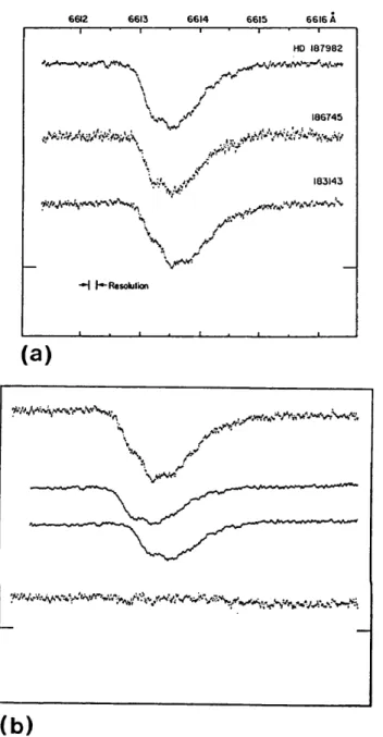
For the high resolution study, data for the sodium D lines and the 66148 diffuse feature were used. The sodium data were used to determine the velocity structure, column densities and velocity dispersions towards each star. The data for the 66148 diffuse feature were used to examine the hypothesis that this diffuse feature is caused by unresolved rotational fine structure within an electronic molecular transition.
Contents
Page
Title Page 1
Abstract 2
Contents 3
List of Tables 9
List of Figures 14
Dedication 22
Chapter 1. INTRODUCTION
1.1 Overview of the Thesis 23
1.2 An Historical Preamble 25
1.3 The Interstellar Environment 28
1.3.1 The Phases of the Interstellar Medium 28 1.3.2 The Nature of the Interstellar Dust 31 1.3.3 Observing the Diffuse Interstellar
Medium 38 1.4 Observations of the Diffuse Interstellar
Features 41
1.4.1 Early Observations 41
1.4.2 Post-war Studies at Moderate Resolution 44
1.4.3 High Resolution Studies 59
1.4.4 Polarisation Studies 62
1.5 Proposed Models of the Production of the
Diffuse Interstellar Features 66 1.5.1 Observational Considerations 66
1.5.2 Gas Phase Models 69
1.5.3 Solid State Models 75
1.5.4 Dust-gas Models 78
1.5.5 General Conclusions 79
1.6 The University of London Observatory Diffuse
Page Chapter 2. DATA ACQUISITION AND REDUCTION
2.1 Overview 82
2.2 The Lick Observatory Observations 82
2.2.1 The Observations 82
2.2.2 The Spectrograph 83
2.2.3 The Mk.II Varo System 84
2.2.4 The Photographic Processing 91 2.2.5 Use of the PDS Facility at the
Royal Greenwich Observatory 92 2.2.6 Computer Software and Data Reduction 95 2.2.7 The Photometric Accuracy 114
2.2.8 The Wavelength Accuracy 121
2.2.9 The Focus Variability 122
2.2.10 Discussion 125
2.3 The Mt. Stromlo Observatory Observations 126
2.3.1 The Observations 126
2.3.2 The Spectrograph 127
2.3.3 The Mt. Stromlo Photon Counting Array 128
2.3.4 The Data Reduction 131
2.3.5 The Photometric Accuracy 135
2.3.6 The Wavelength Accuracy 139
2.3.7 Discussion 141
2.4 Concluding Remarks 142
Chapter 3. STUDIES OF THE DIFFUSE INTERSTELLAR FEATURE AT 6284$
3.1 Overview 144
3.2 Spectroscopic Pollution caused by Telluric
Oxygen 144 3.3 The Telluric Oxygen Alpha Band Rectification
Procedure 153 3.3.1 Outline of the Procedure 153 3.3.2 The Instrumental Response Function 154 3.3.3 Convolution and Interpolation of the
Page 3.4 The Accuracy of the Rectification Procedure 178
3.4.1 General Considerations 178
3.4.2 Statistical Tests 186
3.4.3 Summary 213
3.5 A Comparison with Previous Work on the 6284$
Diffuse Feature 214
3.6 Concluding Remarks 241
Chapter 4. THE SPECTROSCOPIC MEASUREMENTS AND THEIR ERRORS
4.1 Overview 244
4.2 General Considerations 244
4.3 The Measurement of the Central Wavelengths 246 4.4 The Measurement of the Equivalent Widths 249 4.5 The Measurement of the Absorption Depths 261 4.6 Non-random Errors and Non-detection Criteria 264
4.7 Concluding Remarks 268
Chapter 5. A STATISTICAL STUDY OF THE DIFFUSE INTERSTELLAR FEATURES
5.1 Overview 270
5.2 The Data Used 271
5.3 The Computation and Presentation of the
Statistical Results 285 5.4 Univariate Statistical Results 291 5.5 Pollution by Telluric and Stellar
Absorption Lines 298 5.6 Correlations of the Diffuse Features
with Colour Excess 314 5.7 Anomalies in the Strengths of the
Diffuse Features 338 5.8 Correlations between the Strengths of the
Page 5.9 Correlations of the Diffuse Features
with Atomic and Molecular Data 384
5.10 Discussion 419
5.11 Concluding Remarks 425
Chapter 6. HIGH RESOLUTION SPECTROSCOPY OF ATOMIC AND DIFFUSE INTERSTELLAR LINES
6.1 Overview 430
6.2 The Theoretical Basis for Line Profile
Analysis 430
6.2.1 Atomic Absorption Lines 430
6.2.2 The Diffuse Interstellar Features 436 6.3 The Mt. Stromlo Coude Echelle Instrumental
Response Function 440 6.4 The Results of the Sodium D Line Profile
Analysis 448 6.5 The 661$A Diffuse Feature Results 481
6.6 Concluding Remarks 505
Chapter 7. CONCLUSIONS
7.1 Summary of Results 508
7.2 The Cause of the Diffuse Interstellar Features 513 7.2.1 The Observational Evidence 513
7.2.2 The Proposed Models 518
7.2.3 Concluding Remarks 523
7.3 Future Work 524
References
Acknowledgements
Page Appendix 1. GENERAL LEAST SQUARES FITTING OF NON-LINEAR FUNCTIONS
1.1 Introduction 543
1.2 The Grid Search 544
1.3 The Gradient Search 545
1.4 Linearisation 547
1.5 The Gradient Expansion Algorithm 549
1.6 Error Analysis 550
Appendix 2. 2.1
A LISTING OF THE PROGRAM L6284
Introduction 552
2.2 Root Module Listing 552
2.3 SUBROUTINE GFIT Listing 560
2.4 SUBROUTINE PRCYN Listing 572
2.5 SUBROUTINE F6284 Listing 578
2.6 Sample Program Output 588
Appendix 3. 3.1
A REVIEW OF THE STATISTICAL METHODS USED
Introduction 592
3.2 General Considerations 593
3.3 Univariate Statistics 595
3.4 Correlation Statistics 601
3.5 Linear Modelling 607
3.6 Statistical Simulation 618
Appendix 4. 4.1
ADDITIONAL DATA AND STATISTICAL DIAGRAMS
Introduction 622
4.4 Diffuse Feature Measurements Not Used in the Analysis 4.5 Diagrams Used in the Univariate Statistical
Analysis 4.6 Diagrams Used in the Spectroscopic
Pollution Study 4.7 Diagrams Used in the Colour Excess Study
4.8 Diagrams Used in the Diffuse Feature
Anomaly Study 4.9 Diagrams Used in the Diffuse Feature
Inter-relationship Study 4.10 Diagrams Used in the Atomic and Molecular
Correlation Study
Published Papers (inside back c over) :
McNally, D., Ashfield, M . , Baines, D. W . T . , Fossey, S., Rees, P.C.T., Somerville, W.B., & Whittet, D.C.B.,
1985, Astrochemistry (I.A.U. Symposium No. 120), Vardya, M.S., & Tarafdar S.P., (Eds.), Reidel, 321.
Page
644
657
665 674
692
696
709
Crawford, I.A., Rees, P.C.T., & Diego, F.,
List of Tables
1.1 A summary of the McKee & Ostriker (1977) proposed phases of the diffuse interstellar medium. 1.2 Data for all the currently known diffuse interstellar
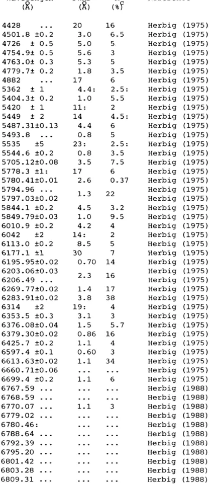
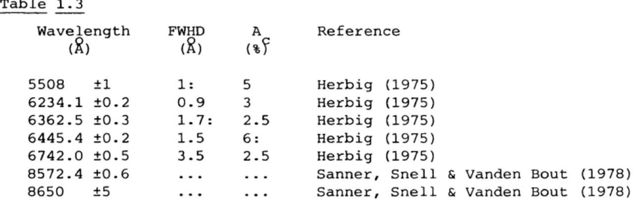
absorption features. 1.3 Data for all the currently suspected diffuse
interstellar absorption features.
2.1 The intensity calibration data used in the
Lick Observatory programme. 2.2 The measured breadths of the 6266$ neon arc line
for the Lick Observatory spectra. 2.3 A comparison of measurements of the 6266$ arc
line made using the Joyce-Loebl Mk.III CS microdensitometer and the Perkin-Elmer PDS
microphotometer.
3.1 A table of oxygen alpha-band components and
their wavelengths. 3.2 A summary of the steps performed in the alpha-band
rectification procedure. 3.3 Error estimates and bench mark timings for
SUBROUTINE GRID. 3.4 A table of measurements of the 6284$ diffuse feature. 3.5 A summary of the statistical results for the
uncorrected and corrected equivalent width data. 3.6 The photometric 6284$ data reported by Murdin (1972). 3.7 The results of correlations including data from
Murdin (1972). 3.8 The 6284$ equivalent width data reported by
Herbig (1975 and 1985). 3.9 Statistical results for the uncorrected and
corrected 6284$ equivalent widths reported
herein and by Herbig (1975 and 1985).
Page
30
45
47
84
123
123
151
155
185 194
208 222
224
228
3.10 Statistical results for all uncorrected and
corrected 6284$ equivalent widths reported herein and by Herbig (1975 and 1985). 3.11 A Comparison between the 6284$ equivalent widths
reported by Schmidt-Kaler et_ a l . (1980) and those reported herein.
4.1 The scatter in the central wavelength measurements. 4.2 An example calculation of the statistical
uncertainty on an equivalent width measurement. 4.3 A comparison between the scatter in the equivalent
width measurements and their estimated uncertainties. 4.4 A comparison between the scatter in the absorption
depth measurements and their estimated uncertainties. 4.5 The non-detection criteria applied to the
diffuse feature measurements.
5.1 General data for each star observed in the Lick
Observatory programme. 5.2 Equivalent width data for all diffuse features
used in the statistical study. 5.3 Mean LSR wavelengths and mean FWHD data for
all the diffuse features measured in the Lick
Observatory programme. 5.4 Univariate statistics for the photometric and
equivalent width data. 5.5 Results for the correlations of the
photometric and equivalent width data with
their associated errors. 5.6 The known telluric lines in the vicinity of
each of the diffuse features. 5.7 The identified stellar lines in the vicinity
of each of the diffuse features. 5.8 Results for the correlations between the
diffuse feature equivalent widths and the intrinsic stellar photometry.
Page
233
239
248
259
260
265
267
274
280
292
297
297
303
304
5.9 Results for the correlations between E(B-V)
and intrinsic (B-V) for each diffuse feature used in the statistical study. 5.10 A table of partial correlation coefficients
for the data presented in Table 5.9. 5.11 Multiple regression results using the diffuse
feature equivalent width as the dependent variable, and E(B-V) and intrinsic (B-V) as the independent
vari ables . 5.12 Results for the correlations between diffuse
feature equivalent width and colour excess for all available data. 5.13 Results for the correlations between diffuse
feature equivalent width and colour excess for
complete data sets only. 5.14 Statistical simulation results for the
correlations presented in Table 5.12. 5.15 Linear least squares fit results for diffuse
feature equivalent width against E(B-V). 5.16 Correlation results for the S(2255) index.
5.17 A summary of the results reported by Snow, York & Welty (1977) for stars showing anomalous
diffuse feature strengths. 5.18 A summary of the anomalous diffuse feature
strengths found in this study. 5.19 Results for the correlations between the diffuse
feature residuals and E(B-V). 5.20 Results for the correlations between the diffuse
feature residuals and stellar intrinsic (B-V). 5.21 A summary of the occurrence of diffuse feature
anomalies in the Lick Observatory data. 5.22 Univariate statistics for the diffuse feature
residuals. 5.23 A summary of the unambiguous diffuse feature
anomalies found in this study. 5.24 A comparison of the diffuse feature anomaly
data with stars known to be associated with
reflection nebulae.
Page
313
313
314
319
321
328
334 336
341
344
349
350
351
353
355
5.25 A comparison of the diffuse feature anomaly
data with stars known to possess dust shells. 5.26 A comparison of the diffuse feature anomaly
data with stars classified as Be stars. 5.27 A comparison of the diffuse feature anomaly
data with stars known to be associated with
H II regions. 5.28 Results for the correlations amongst the
equivalent widths of the diffuse features. 5.29 Results for the correlations amongst the
bivariate diffuse feature residuals. 5.30 Results for the correlations amongst the
trivariate diffuse feature residuals. 5.31 A summary of results for the correlations
amongst atomic and molecular abundance data. 5.32 Results for the correlations between the
abundance data and E(B-V). 5.33 Results for the correlations between
the diffuse feature equivalent widths and the
abundance data. 5.34 A summary of results for the correlations
between the bivariate diffuse feature residuals
and the abundance data. 5.35 A summary of results for the correlations
between the trivariate diffuse feature residuals and the abundance data. 5.36 A summary of the statistically significant
correlations between the diffuse feature residuals and the abundance data.
6.1 A table of data for the Mt. Stromlo coude
echelle spectrograph. 6.2 Atomic data for the sodium D doublet.
6.3 Data for each star observed in the high
resolution study. 6.4 The results of the sodium D line profile analysis.
Page
358
359
360
375
378
380
387
390
394
406
408
411
447 452
Page 6.5 A comparison between the sodium D results
reported by Hobbs (1969 et seq.) and those
reported herein. 6.6 A comparison between the sodium D results
reported by Crawford, Barlow & Blades (1989) and
those reported herein.
7.1 Estimated abundances and transition rates
for the carrier for the diffuse interstellar features.
A3.1 Null hypothesis probabilities and their
interpretation.
A4.1 A table of 6248$ equivalent width data reported
by Herbig (1975 and 1985). A4.2 Johnson photometry for all stars observed in
the Lick Observatory programme. A4.3 TD-1 ultraviolet photometry for all stars
observed in the Lick Observatory programme. A 4 .4 Atomic and molecular abundance data used in the
statistical study. A 4 .5 A table of sodium and potassium abundance data
reported by Hobbs (1978) and herein. A4.6 Mean LSR wavelengths for the diffuse features
studied in the Lick Observatory programme. A4.7 Mean FWHD data for the diffuse features studied
in the Lick Observatory programme. A4.8 Mean absorption depth data for the diffuse
features studied in the Lick Observatory programme.
476
480
520
593
623
626
632
638
642
645
649
List of Figjres
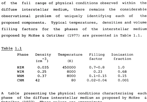
1.1 The interstellar extinction curve from 0 to 10
-1.
microns 1.2 The spectrum of W33A from 1.5 to 14 microns.
1.3 The interstellar spectrum of HD183143 from 5400$ to 6270$. 1.4 Plots of equivalent width against E(B-V) for the
diffuse features at 5780$, 5797$, 6284$ and 6614$. 1.5 The variation of diffuse feature strength per unit
reddening with respect to Galactic longitude. 1.6 High resolution results for the 5614$ diffuse feature
reported by Herbig & Soderblom (1982). 1.7 High signal/noise data in the 6800$ region reported
by Herbig (1988).
2.1 A 6284$ region spectrogram obtained during the
Lick Observatory programme. 2.2 The design of the Varo image intensifier.
2.3 The radial sensitivity curve of the Varo
image intensifier. 2.4 An illustration of pincushion distortion.
2.5 An illustration of "S" distortion.
2.6 The scanning modes of the PDS microphotometer. 2.7 The digitising procedure used for the
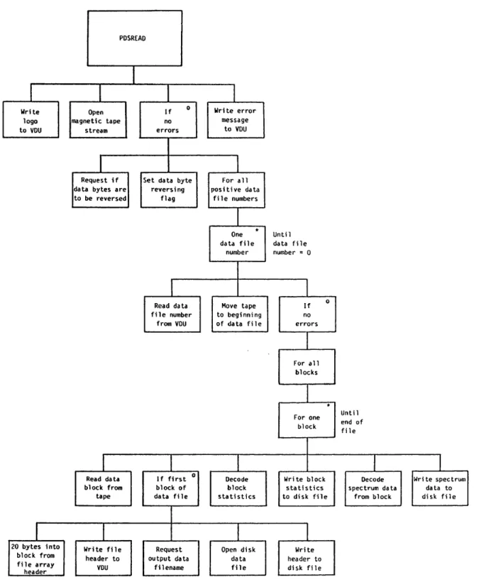
Lick Observatory data. 2.8 The structure of the program PDS R E A D .
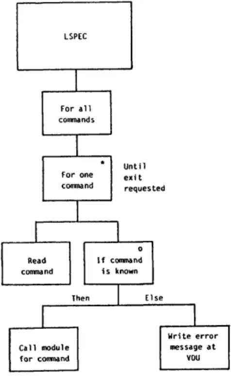
2.9 The structure of the program LICON. 2.10 The structure of the program LWCAL. 2.11 The structure of the program L6284. 2.12 The structure of the program L S P E C .
2.13 Systematic errors in the intensity calibration
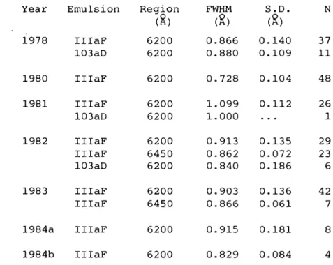
applied to the Lick Observatory data. 2.14 Signal/noise characteristics of the IIIaF and
103aD emulsions. 2.15 An unrectified spectrum taken with the
1-dimensional PCA.
J. o
2.16 Raw spectrum images taken with the 2-dimensional PCA. 2.17 Unrectified spectra extracted from 2-dimensional
PCA images. 2.18 A flat field image taken with the 2-dimensional PCA. 2.19 Signal/noise characteristics of spectra taken with
the 1-dimensional PCA. 2.20 Signal/noise characteristics of spectra extracted
from 2-dimensional PCA data.
3.1 The effect of the alpha-band of telluric oxygen
upon the 6248^ diffuse feature. 3.2 A high resolution spectrum of the oxygen alpha-band
from the Procyon data of Griffin & Griffin (1979). 3.3 The identification and rectification of stellar lines
in the alpha-band data of Griffin & Griffin (1979). 3.4 A flow chart of the alpha-band rectification
pr o c e d u r e . 3.5 The structure of the alpha-band rectification
program L6284. 3.6 The data plotted at the terminal during the
alpha-band rectification procedure. 3.7 Several fits of the 6266$ neon arc line
to a Gaussian function calculated during the
alpha-band rectification procedure. 3.8 Flow charts illustrating the rigorous and the
adopted procedures used to account for the
instrumental response function. 3.9 Systematic errors resulting from the procedure used
to account for the instrumental response function. 3.10 Examples of the results of the rectification
procedure for stars of low reddening. 3.11 Plots of optical depth scaling factor against
air mass and E(B-V). 3.12 Frequency bar charts for the air mass data.
3.13 An illustration of the equivalent width
measurement procedures used. 3.14 Plots of the 6284^ equivalent widths against
E(B-V) for the uncorrected and corrected data.
3.15 Plots of the 6284$ equivalent widths against
log(air mass) for the uncorrected and corrected data. 3.16 Plots of the 6284$ equivalent widths against
log(optical depth scaling) for the uncorrected
and corrected data. 3.17 Plots of log(optical depth scaling) against
log(air mass) for the June/July data and
the September/October data. 3.18 Examples of the rectification results for several
reddened stars. 3.19 Plots of the uncorrected and corrected 6284$
equivalent widths and the Murdin (1972) 6284$
index against E(B-V). 3.20 Plots of the uncorrected and corrected 6284$
equivalent widths against the Murdin (1972)
6284$ index. 3.21 An illustration of the equivalent width measurement
procedures used by Herbig (1975 and 1985). 3.22 Plots of the 6284$ equivalent widths against
E ( B - V ) for the uncorrected data, the corrected
data and the data of Herbig (1975 and 1985). 3.23 Plots of corrected against uncorrected 6284$
equivalent widths for the data reported herein
and those reported by Herbig (1975 and 1985). 3.24 Plots comparing the uncorrected 6284$ equivalent
widths reported herein with those of Herbig (1975), and the corrected 6284$ equivalent widths reported
herein with those reported by Herbig (1985). 3.25 Plots of the 6284$ equivalent widths against
E(B-V) for all the data reported herein and by
Herbig (1975 and 1985). 3.26 Plots of corrected against uncorrected 6284$
equivalent widths for all the data reported herein and by Herbig (1975 and 1985). 3.27 A plot of the 6284$ equivalent widths reported
by Chlewicki ^t. a l . (1986) against E(B-V).
Page
207
209
212
215
223
225
227
230
232
234
236
237
4.1 An illustration of equivalent width measurement for discretely sampled data.
5.1 Example plots of all diffuse features used in the statistical study. 5.2 Frequency bar charts for the photometric data used
in the statistical study. 5.3 Frequency bar charts for the equivalent width data
used in the statistical study. 5.4 Plots of the standard error on the colour excess
data against colour excess. 5.5 Plots of the standard error on the equivalent
width data against equivalent width. 5.6 Example plots of the diffuse feature equivalent
widths against intrinsic colour index. 5.7 Frequency bar charts for spectral type and
luminosity class for all stars observed. 5.8 The relationship between intrinsic colour index
and My for a star of spectral type B2. 5.9 Plots of E(B-V) against intrinsic colour excess
for the 6284A diffuse feature data set. 5.10 Plots of colour excess against colour excess
for all colour excess data used in the statistics, o
5.11 Plots of the 6284A diffuse feature equivalent
width against colour excess. 5.12 Plots of diffuse feature equivalent width
against the E(B-V) colour excess. 5.13 Plots of the S(2255) index against E(B-V) and
the 6284^ diffuse feature equivalent widths. 5.14 A frequency bar chart for the S(2255) index data. 5.15 Frequency bar charts for the equivalent width
residuals of the 578oS and 6284^ diffuse features. 5.16 Plots of standardised bivariate diffuse feature
residuals against Galactic longitude. 5.17 Plots of standardised trivariate diffuse feature
residuals against Galactic longitude. 5.18 Example plots of several anomalous diffuse
feature spectra.
5.19 A Venn diagram showing the inter-relationships
between the diffuse features. 5.20 Example plots of log(column density)
against log(column density) for the abundances
used in the study. 5.21 Example plots of log(abundance ratio) against E ( B-V) . 5.22 Example plots of diffuse feature equivalent
width against log(abundance ratio). 5.23 Plots of the diffuse feature equivalent width
residuals against log N ( C H ) . 5.24 Plots of the diffuse feature equivalent width
residuals against log N(Ca+ )/N(H).
6.1 The definition of the coordinate system local
to a diffraction grating. 6.2 An example of the instrumental response function
of the Mt. Stromlo coude echelle spectrograph. 6.3 The observed profiles of the 6328$ helium/neon
laser line. 6.4 The observed profiles of the 5770$ mercury line.
6.5 The sodium D2 spectra observed towards each star
used in the high resolution study. 6.6 A comparison of the observed sodium Dl and D2
spectra towards the stars HD144217 and HD149757. 6.7 The results of the sodium line profile analysis
for the stars HD149757 and HD152236. 6.8 The observed relationship between the estimated
velocity dispersion and column density. 6.9 An illustration of the fits corresponding to the maximum
acceptable sodium column density towards HD144217. 6.10 The observed profiles of the 6614$ diffuse
interstellar feature. 6.11 Detailed plots of the 6614$ diffuse feature
towards the stars HD144217 and HD149757. 6.12 Plots of the 6614$ diffuse feature towards
the stars HD144217 and HD149757 after smoothing. 6.13 The 6614$ diffuse feature profile reported by
Herbig & Soderblom (1982) .
19
6.14 The results of modelling the profile of the
6614$ diffuse feature using a linear molecule. 6.15 Further results of modelling the profile of the
6614$ diffuse feature using a linear molecule. 6.16 The results of modelling the profile of the
6614$ diffuse feature using a symmetric top molecule. 6.17 Some simple polycyclic aromatic hydrocarbons.
6.18 The effects of spectrograph resolution
on the observed rotational fine structure of a
symmetric top molecule.
Al.l A flow chart of the gradient expansion algorithm of Marquardt (1963).
A3.1 The shapes of distributions with non-zero
coefficients of skewness and kurtosis.
A4.1 A plot of the relationship between the interstellar column densities of sodium and potassium. A4.2 Frequency bar charts for all the intrinsic
stellar photometry used in the statistical study. A4.3 Frequency bar charts for all colour excess data
used in the statistical study. A4.4 Frequency bar charts for all equivlalent width
data used in the statistical study. A4.5 Plots of standard error against colour excess for
all colour excess data used in the statistical study. A4.6 Plots of standard error against equivalent
width for all equivalent width data used in the
statistical study. A4.7 Plots of diffuse feature equivalent width
against the stellar intrinsic (U-B) colour index. A4.8 Plots of diffuse feature equivalent width
against the stellar intrisic (B-V) colour index. A4.9 Plots of the E(U-B) colour excess against the
stellar intrinsic (U-B) colour index. A4.10 Plots of the E(B-V) colour excess against the
stellar intrinsic (B-V) colour index.
Page
495
496
499 501
503
551
600
643
658
659
660
662
663
666
668
670
20
A4.ll Plots of colour excess against colour
excess for all colour excess data used in the
statistical study. A4.12 Plots of the diffuse feature equivalent widths
against the E{1565-V) colour excess. A4.13 Plots of the diffuse feature equivalent widths
against the E{2255-V) colour excess. A4.14 Plots of the diffuse feature equivalent widths
against the E(2475-V) colour excess. A4.15 Plots of the diffuse feature equivalent widths
against the E(U-V) colour excess. A4.16 Plots of the diffuse feature equivalent widths
against the E(U-B) colour excess. A4.17 Plots of the diffuse feature equivalent widths
against the E(B-V) colour excess. A4.18 Plots of the S(2255) index against the Johnson
colour excess data used in the statistical study. A4.19 Plots of the diffuse feature equivalent
widths against the S(2255) index.
A4.20 Frequency bar charts for the diffuse feature
equivalent width residuals. A4.21 Plots of the diffuse feature equivalent widths
against the diffuse feature equivalent widths. A4.22 Plots of the bivariate diffuse feature residuals
against the bivariate diffuse feature residuals. A4.23 Plots of the trivariate diffuse feature residuals
against the trivariate diffuse feature residials. A4.24 Plots of log(column density) against
log(column density) for all abundance data
used in the statistical study. A4.25 Plots of log(column density) against the
E(B- V) colour excess. A4.26 Plots of log(abundance ratio) against the
E (B-V) colour excess. A4.27 Plots of all statistically significant
correlations between the diffuse feature
strengths and log(column density).
A4.28 Plots of all statistically significant correlations between the diffuse feature
strengths and log(abundance ratio). A4.29 Plots of diffuse feature strength against log N(H). A4.30 Plots of the diffuse feature residuals
against abundance index where both bivariate and trivariate residuals yield statistically
significant correlations. A4.31 Plots of the diffuse feature residuals
against abundance index where only the bivariate residuals yield statistically
significant correlations. A4.32 Plots of the diffuse feature residuals
against abundance index where only the trivariate residuals yield statistically
significant correlations.
722 723
725
729
22
J o u r n e y 's End
Christopher, Christopher, where are you going, Christopher Robin? "Just up to the top of the hill,
Upping and upping until
I am right on the top of the hill," Said Christopher Robin.
Christopher, Christopher, why are you going, Christopher Robin? There's nothing to see, so when
You've got to the top, what then? "Just down to the bottom again,"
Said Christopher Robin.
A. A. Milne
With love to my parents
Chapter 1
INTRODUCTION
1.1 Overview of the Thesis
Chapter 1 presents a review of previous investigations into the diffuse interstellar features against a background of studies of the diffuse interstellar medium. After briefly reviewing the observational and physical nature of the diffuse interstellar medium, previous observational studies of the diffuse interstellar features are discussed. This is followed by a review of the theoretical studies of the cause of the diffuse features. The chapter is concluded with a brief outline of the approach to studying the diffuse interstellar features adopted in this thesis.
Chapter 2 discusses the instrumental details of the observations made at the Lick and Mt. Stromlo Observatories. This chapter also discusses the procedures used in the reduction of the data from these observatories and the resultant accuracy of the photometric and wavelength calibrations. The estimates of accuracy derived in this chapter are of central importance to the error analysis presented in Chapter 4.
o Chapter 3 discusses the spectroscopic pollution of the 6284A diffuse interstellar feature by the alpha band of telluric molecular oxygen. The method of correction of this pollution, as applied to the Lick Observatory data, is then discussed and the results for the 6284^ diffuse feature examined. The accuracy of the computational procedure is discussed in some detail, both from a computational and a statistical aspect. The chapter ends with a comparison between the results of this work and existing published data for the 6284^ diffuse feature.
Chapter 5 reports a thorough bivariate statistical study of the diffuse interstellar features at 5780$, 5797$, 6196$, 6203$, 6270$, 6284$ and 6379$, using data obtained at the Lick Observatory. After a brief discussion of the content of the data acquired from the published literature and included in the statistical analysis, the results of the statistical study are presented. These results include:
o an examination of the effects of spectroscopic pollution of the diffuse features by the stellar and telluric spec t r a ;
o an examination of the relationship between the strengths of the diffuse features and interstellar reddening, using both visual and ultraviolet measures;
o an examination of the existence and nature of any anomalies in the strengths of the diffuse interstellar features with respect to reddening;
o an examination of the relationships among the strengths of the diffuse features;
o an examination of the relationship between the strengths of the diffuse features and atomic and molecular abundances.
The chapter concludes with a discussion of the statistical results and an attempt to establish a basis for the physical interpretation of the statistical results.
25
possible molecular band component separation within the diffuse feature.
The thesis is concluded with Chapter 7, which summarises the findings of the previous chapters. This chapter also attempts to criticise the weaknesses of the current work and to suggest ways in which these weaknesses may be overcome in future work- Some suggestions of the most informative directions that future research programmes might take are also presented.
1.2 An Historical Preamble
The use of spectroscopy as a scientific tool to obtain physical information about astronomical phenomena has been of singular importance in the development of modern astrophysics. Perhaps the credit for performing the first spectroscopic investigations may be awarded to Sir Isaac Newton for his experiments in 1672, dispersing sunlight with prisms. After Newton, it was not until the first decade of the nineteenth century that further contributions to our understanding of spectroscopy and the nature of spectra began to be made.
The first of these contributions was the extension of the known visual spectrum beyond the extremes to which the human eye is sensitive. In 1800, William Herschel demonstrated the existence of rays beyond the red end of the solar spectrum, the infra-red, by using a thermometer as a means of detection. In 1801, J.W. Ritter confirmed the existence of a similar region beyond the violet end of the solar spectrum, the ultra-violet, using the blackening of silver chloride as a means of detection.
attributed these lines to be the natural boundaries between the different colours and did not pursue the investigation any further. He also noted the difference between the continuous character of the solar spectrum and the discrete character of the candle spectrum. Since this was the first recorded observation of an emission spectrum these results caused some learned discussion concerning the fundamental nature of the candle flame spectrum.
The first modern spectroscope to be constructed was reported by J. Fraunhofer in 1817. In this paper, Fraunhofer also reported his spectroscopic observations of the Sun, planets and stars. Fraunhofer's observations of the solar spectrum were the first to systematically document the solar absorption lines which have since taken his name. He documented a total of 354 dark lines in the solar spectrum, among them the very strong D line. Fraunhofer also discussed the nature of these lines and reported his view that the D line corresponded exactly in wavelength to the bright emission line observed in lamp flames. His observations of the the Moon and the planets Venus and Mars verified that their spectra were essentially the same as that of sunlight. Observations of the bright stars Sirius, Castor, Pollux, Capella, Betelgeux and Procyon demonstrated the nature of stellar spectra generally to be different to that of the Sun.
Within the following two decades contributions to spectroscopy were made by J.W.H. Herschel (1823), Brewster (1832 and 1834) and Fox Talbot (1834). In particular, Fox Talbot was probably the first to begin to explore the potential of spectroscopy as an analytical tool in the study of chemical composition. This potential was further explored by Wheatstone (1835) using electric sparks to generate the emission spectra of m e t a l s .
In the 1850's, the use of spectroscopy as a tool for chemical analysis was substantiated, first by Angstrom and later by Kirchhoff & Bunsen (1860), in comparative laboratory and solar studies. Kirchhoff (1861), in discussing the relationship between emission and absorption spectra, also began to establish these qualitative studies on a more profound physical basis. However, the precise physical nature of spectra was only elucidated in the early years of the twentieth century.
work of Bunsen and Kirchhoff and their predecessors to the investigation of astronomical phenomena. In his early studies, Huggins collaborated with W.A. Miller and succeeded in taking the first photographic astronomical spectra of several first magnitude stars. In the following year, Huggins went on to observe the emission line spectra of gaseous nebulae, establishing the existence of two uniquely different types of nebulae: those with emission spectra, and those with continua and absorption spectra. One further innovation made by Huggins was the measurement of the shift of stellar spectral lines as a result of the Doppler effect. The first measurement of this kind was made soon after 1868 using the spectrum of Sirius.
Although a spectroscopic classification scheme had been suggested by L.M. Rutherford as early as 1863, it was Secchi (1866a, b) who first suceeded in cataloguing stars according to such a classification scheme. Further work on stellar spectral classification was initiated by H. Draper some time later. This work was continued after his death by E.C. Pickering to produce a classification of variable stars (1881); to develop the use of telescope objective prisms and photographic plates to obtain many spectroscopic observations simultaneously (1886); and to discover spectroscopic binary stars (1890).
1.3 The Interstellar Environment
1.3.1 The Phases of the Interstellar Medium
In addition to the observation of absorption lines arising from gas in the interstellar environment, it has also been apparent that localised regions of gas exist which radiate light at discrete wavelengths - the H II regions. Although these nebulae have been known since the work of Huggins in the late 19th Century, their precise interstellar nature only became clear in the 20th Century. As early as the late 18th Century W. Hershel noted the patchiness in the apparent distribution of stars in the Milky Way. Barnard (1927) published a photographic atlas of selected regions of the Milky Way which illustrated the cloud like nature of these dark nebulae. Associated studies by V.M. Slipher prompted H.N. Russell in correspondence with H. Shapley (Seeley & Berendzen, 1972) to suggest a dust origin for both the dark nebulae and the blue reflection nebulae in which the size of the dust particles was proposed to be similar to the wavelength of visible light. However, the dust origin of these nebulae was not substantiated until Trumpler (1930) demonstrated both the existence and the precise wavelength dependence of interstellar extinction. Interstellar astrophysics has since studied the composition and physical state of both these components of the interstellar medium - gas and dust.
The physical state of the interstellar medium is characterised by the state of the interstellar gas. By considering the thermal equilibrium of the interstellar medium using radiative cooling and heating by cosmic rays, Field, Goldsmith & Habing (1969) proposed a two phase model of the inte rstellar.medium in which two physically distinct phases exist in pressure equilibrium. These two phases are: cool neutral
-3
diffuse clouds with densities around 20cm and temperatures around 80K; a warm intercloud medium with a density and
-3
29
-17 -1
rate derived from Copernicus observations (e.g. 10 s ; Black & Dalgarno, 1977) suggest this model to be untenable. In addition, in the two phase model, the interstellar medium cannot be maintained in a steady state if more recent rates of supernova explosions are realistic (e.g. McKee & Ostriker, 1977). Also, no observational evidence for the warm intercloud medium has been found, and the mean electron density of the interstellar medium derived from pulsar dispersion measurements (e.g. Kulkarni & Heiles, 1987) is inconsistent with the proposed warm intercloud medium. Finally, the existence of a phase of the interstellar medium at coronal temperatures, suggested by O VI absorption in the ultraviolet (e.g. Jenkins, 1978) and a soft X-ray background (e.g. Burnstein et_ a l ., 1976), cannot be explained by the model of Field, Goldsmith & Habing.
McKee & Ostriker (1977) proposed a "three phase" model of the interstellar medium in which supernova explosions in a cloudy medium constitute the major energy source. Their proposed phases of the interstellar medium are as follows:
(i) Cold Neutral Medium (CNM) - the cold cores of interstellar clouds;
(ii) Warm Neutral Medium (WNM) - the warm neutral envelopes of c l o u d s ;
(iii) Warm Ionised Medium (WIM) - the partially ionised cloud en v e l o p e s ;
(iv) Hot Ionised Medium (HIM) - the hot, low density cavities of supernova remnants.
This theory is able to satisfactorily explain the observed mean electron densities in the interstellar medium, the observed soft X-ray background, the observed cloud velocity dispersion and the
-3
of the full range of physical conditions observed within the diffuse interstellar medium, there remains the considerable observational problem of uniquely identifying each of the proposed components. Typical temperatures, densities and volume filling factors for the phases of the interstellar medium proposed by McKee & Ostriker (1977) are presented in Table 1.1.
Table 1.1
Phase Density (cm )
Temperature (K)
Filling factor
Ionisation fraction
HIM 0.035 450000 o r- 1 0 00 1.0
WIM 0.25 8000 0.23 0.68
WNM 0.37 8000 0.1-0.15 0.15
CNM 42 80 0.02-0.04 0.001
A table presenting the physical conditions characterising each phase of the diffuse interstellar medium as proposed by McKee & Ostriker (1977). These values are approximate.
In the physical description of the phases of the interstellar medium little has been mentioned about morphologically distinct phenomena such as H II regions, reflection nebulae, dark nebulae and molecular clouds. Generally, these phenomena all occur at higher densities than those typified by diffuse interstellar clouds. H II regions occur in the vicinity of main-sequence 0 stars and are regions of photo ionised hydrogen. Their presence is indicated by H I and 0 III emission lines in the visible spectrum. Typical densities for
2 - 3 3 - 3
H II regions range from 10 cm to 10 cm and temperatures for these objects are around 8000K. Although observationally very distinct, H II regions are highly localised, having a volume filling factor which is diminishingly small with respect to diffuse clouds. Dark matter and observational molecular clouds are often coincident. Observational indicators for molecular clouds are commonly CO, OH or H CO radio emission. Typical
2 - 3 7 - 3
clouds are chemically active and produce simple molecules, e.g. +
CO, CH, CH , CN (Black & Dalgarno, 1977; Dickman et: a l . , 1983; Mann & Williams, 1984 and 1985). However, the giant molecular clouds have a volume filling factor of less than 1% and appear to have an environment closely related to the galactic spiral structure. This behaviour is also true for the distribution of H II regions.
The four phases or domains of the diffuse interstellar medium simplistically suggest a spherical symmetry to a diffuse cloud, i.e. a cold cloud core successively enveloped in a warm neutral medium, a warm partially ionised medium, and embedded in a hot ionised medium. McKee & Ostriker give typical dimensions for each of these domains (see Table 1.1). They also suggest that the clouds will only become distorted from a roughly spherical symmetry on interaction with the shell of a supernova remnant. Observationally, however, diffuse interstellar clouds do not appear to be spherical but more sheet-like or filamentary (e.g. Kulkarni & Heiles, 1987). This may have important implications for the interpretation and modelling of physical processes within diffuse interstellar clouds.
1.3.2 The Nature of the Interstellar Dust
There are five major observational indications of the existence of dust in the interstellar medium: dark nebulae, reflection nebulae and the diffuse galactic light, interstellar extinction, the polarisation of starlight, infra-red thermal emission. In addition, the existence of the depletion of several elements in the gas phase in diffuse interstellar clouds has been interpreted as evidence for the presence of these elements in grain materials. The existence of infra-red absorption and emission features (e.g. Aitken, 1981) also suggests the existence of silicates as a grain material in the interstellar medium and water ice as a grain mantle component in dense interstellar regions. These observations have been reviewed by Savage & Mathis
(1979) and Whittet (1981).
10
>I
m W
10
8 6
0 2 4
1 / A in y u m 1
Figure 1.1
0 microns ^ to 10 microns ^ in units of reciprocal wavelength. It can be seen from this figure that the broad trend of interstellar extinction is roughly inversely proportional to wavelength. In addition to this broad behaviour, there also exists structure in the extinction curve. The most notable feature is in the ultraviolet region at an approximate wavelength of 22008. The width of this feature is approximately 0.2 in units of dX/X. In the visible region, the diffuse interstellar features may also be regarded as fine structure (e.g. York, 1971; Herbig, 1975). The widths of the diffuse features range from 0.005 to 0.0001. The visible spectrum also exhibits very broad band extinction structure (Whiteoak, 1966; Hayes et a l ., 1973; van Breda & Whittet, 1981) with widths upwards of 0.02 and typically 0.1. In the infra-red region, common absorption features are found at wavelengths of 3.07 microns and 9.7 microns. These features have widths of approximately 0.15 and 0.5 respectively. Other infra red absorption features also exist.
The interpretation of the 220oX feature has been the subject of considerable investigation since the early ultraviolet observations reported by Stecher (1965). The feature, which has its central wavelength near 2175^, has customarily been interpreted as a pure absorption feature resulting from a distribution of small carbon grains (e.g. Mathis, Rumpl & Nordsieck, 1977; Draine & Lee, 1984). More recently, Steel & Duley (1987) have presented laboratory results which indicate that small silicate particles also have an absorption peak near 2175^. Duley (1987) and Duley, Jones & Williams (1989) have suggested a dust model which incorporates silicate particles coated with hydrogenated amorphous carbon, where the 220o£ feature is produced by small magnesium-rich silicate grains. In particular, this model is able to explain the variations in the ultraviolet extinction curve reported by Savage (1975), Massa, Savage & Fitzpatrick (1983), Massa & Fitzpatrick (1986) and Carnochan (1986) simply by carbon depletions.
Although the reality of very broad band structure in the interstellar extinction curve is no longer in doubt, the processes likely to produce such structure are still the subject of some discussion. Van Breda & Whittet (1981) reviewed the possible causes of this structure and concluded that the most likely cause is the existence of magnetite (Fe^O^) within the particles responsible for the extinction and polarisation in the visible region. The nature of the diffuse features, however, remains a subject of continuing investigation after over 50 y e a r s .
also been interpreted as being due to bending of the Si-O-Si bond in silicates. The 3.07 micron feature has been interpreted as being due to water ice within grain mantles. Impurities in this ice, from NH^ and hydrocarbons, may be invoked to explain the variations observed in the profile of this feature. Also, the shape of this feature may be affected by stretching vibrations in the C-H bond, expected to occur between 3.3 and 3.5 microns. Other absorption features occur at 4.61, 6.0 and 6.8 microns and remain unidentified. Figure 1.2 illustrates the spectrum of the heavily reddened infra-red source W33, in the wavelength range 2 to 14 microns. Furthermore, emission features occur at 11 microns, attributed to SiC, and at 3.28, 3.4, 3.5, 6.2, 7.7, 8.6 and 11.3 microns. The latter features are understood to arise at the interface between H I and H II regions but are otherwise unidentified.
Whittet (1984) reviewed the available atomic depletion data, derived mainly from ultraviolet observations. He noted that the carbon depletion in diffuse interstellar clouds is usually 30%, but can lie in the range 0% to 65%, and that the precise depletion is dependent upon the density within the cloud. Since the production of CO in these clouds accounts for only a small fraction of this depletion, the carbon depletion implies the presence of some form of carbon in grains or grain mantles. Whittet adopted a typical depletion of 40% for oxygen and nitrogen in diffuse clouds. For silicon and the metals, he noted that iron is depleted by an average of 98% and that the metals aluminium, titanium, nickel and calcium show higher depletions. However, zinc remains relatively undepleted. The depletions of iron, aluminium and calcium show significant correlations with cloud density and all the metals correlate loosely with condensation temperature. From an analysis of these depletion data, Whittet concluded that silicates and metal oxides are the dominant grain materials.
xj \J
W 3 3 A
450 K
- 1 6
I
3.07 . 4.61 6.06.8 <M
£ o -1 7
ii.
1.5 2 3 4 6 8 10 12 14
X (/im)
Figure 1.2
Diagram illustrating the spectrum of the heavily reddened infra red source W33A in the wavelength range 1.5 microns to 14 microns
region. When the wavelength dependence of polarisation is normalised, relative to the wavelength of maximum polarisation, all such curves show close agreement to a single empirical relationship (Serkowski, Mathewson & Ford, 1975). These observations suggest a constant grain refractive index for the grains responsible for the polarisation in the blue to the near infra-red. Mathis (1979) suggested that these polarising grains are dielectric and have the same size distribution as those responsible for the extinction at visible wavelengths. This, in turn, suggests that the population of small grains normally adopted to explain the extinction in the ultraviolet are either spherical in shape or unaligned.
Infra-red thermal emission from interstellar dust results from the absorption of ultraviolet or visible photons and the subsequent emission of this energy as longer wavelength radiation. Generally, the absorption of a photon of light will increase the grain temperature smoothly. However, if the grain is small, of radius less than 0.01 microns say, then the grain will experience large fluctuations in temperature because of the heating effect of a single photon on such a small quantity of material. In dense interstellar environments, grain heating by collisions with atoms and molecules also becomes an important heating mechanism. However, in diffuse interstellar clouds, grain heating is predominantly radiative.
surfaces (e.g. Duley & Millar, 1978); the chemical adsorption of refractory elements onto grains (e.g. Barlow, 1978c) .
Grain destruction in the diffuse interstellar medium is dominated by the effects of interstellar shocks. Three mechanisms for the destruction of grains by shocks exist: thermal sputtering by a hot gas; non-thermal sputtering by the acceleration of grains; collisions between accelerated grains. The latter two processes occur only in shocks which are radiative.
1.3.3 Observing the Diffuse Interstellar Medium
In addition to the density and temperature of interstellar clouds, several other physical parameters are of considerable importance to their observational appearance: the ambient interstellar radiation field; elemental abundances; grain composition and abundance; the cosmic ray ionisation rate; the cloud geometry. These parameters in turn influence chemical processes, both two-body gas phase and grain surface reactions, and grain composition. Theoretical studies of the chemistry of diffuse interstellar clouds indicate that these clouds are typically in chemical equilibrium and that the chemistry is dominated by radiative ionisation and dissociation processes
(e.g. Duley & Williams, 1984).
The effect of interstellar shocks upon diffuse clouds is to introduce a time-dependent change in the physical conditions within the cloud away from those suggested by steady-state models. Shocks to neutral interstellar gas may arise at the boundaries of H II regions, from collisions between diffuse clouds, from density waves associated with Galactic spiral structure, and from supernova explosions. The incidence of a shock will generally lead to a local increase in cloud density and temperature and also accelerate the gas to a velocity close to that of the shock front. The precise physical behaviour of the shocked region will be dependent upon whether the gas has time to maintain radiative equilibrium (i.e. low velocity shocks) and whether local magnetic fields are significant (e.g. Shull & Draine, 1987).