Journal of Open Innovation: Technology, Market, and Complexity
Article
Modified Di
ff
erential Evolution Algorithm for a
Transportation Software Application
Naratip Supattananon and Raknoi Akararungruangkul *
Department of Industrial Engineering, Faculty of Engineering, KhonKaen University, KhonKaen 40000, Thailand; [email protected]
* Correspondence: [email protected]
Received: 16 August 2019; Accepted: 10 October 2019; Published: 12 October 2019
Abstract:This research developed a solution approach that is a combination of a web application and the modified differential evolution (MDE) algorithm, aimed at solving a real-time transportation problem. A case study involving an inbound transportation problem in a company that has to plan the direct shipping of a finished product to be collected at the depot where the vehicles are located is presented. In the newly designed transportation plan, a vehicle will go to pick up the raw material required by a certain production plant from the supplier to deliver to the production plant in a manner that aims to reduce the transportation costs for the whole system. The reoptimized routing is executed when new information is found. The information that is updated is obtained from the web application and the reoptimization process is executed using the MDE algorithm developed to provide the solution to the problem. Generally, the original DE comprises of four steps: (1) randomly building the initial set of the solution, (2) executing the mutation process, (3) executing the recombination process, and (4) executing the selection process. Originally, for the selection process in DE, the algorithm accepted only the better solution, but in this paper, four new selection formulas are presented that can accept a solution that is worse than the current best solution. The formula is used to increase the possibility of escaping from the local optimal solution. The computational results show that the MDE outperformed the original DE in all tested instances. The benefit of using real-time decision-making is that it can increase the company’s profit by 5.90% to 6.42%.
Keywords: vehicle dispatching problem; inbound transportation problem; modified differential evolution algorithm
1. Introduction
The Internet of Things, cloud technology, big data, and web and mobile applications are technologies used to increase the efficiency of the supply, production, and transportation chains. They allow for the application of information technology (IT) to current management knowledge. The data required to achieve successful decision-making are obtained from IT and used by decision-makers to make more effective real-time decisions to gain the maximum profit for the company.
Nowadays, IT is widely used in transportation management, such as for the application of the geographic information system (GIS) in truck tracking systems, automatic inventory management systems, online procurement systems, and so forth. In this research, we apply an IT system that supports a company’s transportation planning so that the depot will send vehicles to pick up finished goods from production plants, and sometimes the depot has to send trucks to pick up raw materials from suppliers and deliver them to production plants. During the working day, or the planning period, the demand from suppliers and the amount of finished goods may change, which can affect the current transportation plan. This happens because of new demands from the production plant, the capacity of trucks may be not suitable for the new demand, the current positions of trucks can be rerouted if new
information appears in the system, and so forth. The problem statement explained above is known as the vehicle dispatching problem (VDP).
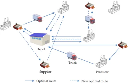
Figure1shows the original optimal route at the beginning of the plan. After the producer or the supplier provides new information to the depot, the new optimal travel plan for the trucks will be released and the trucks will receive the information regarding changing their routes. Trucks will get the information of new routes when they arrive at their current destination. If there is no change, then drivers will continue driving to the next destination, where they get the latest information from the depot.
rerouted if new information appears in the system, and so forth. The problem statement explained above is known as the vehicle dispatching problem (VDP).
Figure 1 shows the original optimal route at the beginning of the plan. After the producer or the supplier provides new information to the depot, the new optimal travel plan for the trucks will be released and the trucks will receive the information regarding changing their routes. Trucks will get the information of new routes when they arrive at their current destination. If there is no change, then drivers will continue driving to the next destination, where they get the latest information from the depot.
Figure 1. Example of the original route at period 0 and new optimal route after new information is obtained during truck operation.
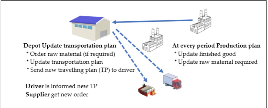
At the beginning of the planning period, all pickup and delivery transportation plans will be given to the truck drivers. They will start their work with the current transportation plan. The information for decision-makers to use as the data for reoptimizing the transportation plan comes during the working period (within the transportation planning horizon). The trucks will get the information for a new route if they need to change their next destination when they arrive at their current destination. The information (e.g., quantity of finished goods available to be picked up and new demand for raw material from the supplier) is updated from the production plants. This information will be transferred to the depot, which will use the proposed method to solve the problem. In the case of increased profit, the new transportation plan will be sent to drivers using the web application, but if the profit is not increased, drivers will not be informed, and they will continue driving according to their current plan. Figure 2 explains how the information flows during the reoptimization process.
Apart from the use of information technology, the depot calculates the daily optimal travel plan for drivers and lets them drive their trucks until the daily plan is finished. Using information technology, the travel plan can be reoptimized to generate better profits than would be achieved with the original version of the travel plan. The transportation plan will support the production line to have enough raw material to support the production plan. The supplier can generate more profit due to the ability to sell more raw materials, and this system will represent a significant innovation for
Figure 1. Example of the original route at period 0 and new optimal route after new information is obtained during truck operation.
At the beginning of the planning period, all pickup and delivery transportation plans will be given to the truck drivers. They will start their work with the current transportation plan. The information for decision-makers to use as the data for reoptimizing the transportation plan comes during the working period (within the transportation planning horizon). The trucks will get the information for a new route if they need to change their next destination when they arrive at their current destination. The information (e.g., quantity of finished goods available to be picked up and new demand for raw material from the supplier) is updated from the production plants. This information will be transferred to the depot, which will use the proposed method to solve the problem. In the case of increased profit, the new transportation plan will be sent to drivers using the web application, but if the profit is not increased, drivers will not be informed, and they will continue driving according to their current plan. Figure2explains how the information flows during the reoptimization process.
J. Open Innov. Technol. Mark. Complex.2019,5, 84 3 of 15 J. Open Innov. Technol. Mark. Complex.2019, 5, x FOR PEER REVIEW 3 of 15
many supply chain businesses, thus it will become an example of supply chain 4.0 and the idea of “smart transportation” will be implemented in many organizations.
This paper is organized as follows: Section 2 presents the literature review, which describes papers related to this research. Section 3 presents the mathematical model formulated for the problem used in the reoptimization process. The proposed methods are shown in Section 4, while Sections 5 and 6 present the computational results and conclusion, respectively.
Figure 2. Information flow during the reoptimization process.
2. Literature Review
Transportation costs form a major proportion of the total costs incurred by any factory or production and distribution organization. They not only affect the company’s overall costs and profits, but are also related to fuel use, which can affect the global warming problem. Addressing this issue can enhance the reputation of an organization, as well as increase profits. Accordingly, transportation cost is the first cost item that many organizations focus on when seeking to reduce expenditures.
The term “taxi dispatching problem” (TDP) has arisen to identify the modern transportation problem. Most of the research is focused on using the Internet of Things to manage requests for taxis from customers while maximizing profitability for drivers [1]. A driver’s profit is controlled by the idle time of the taxi during the working time. The taxi must respond immediately to passenger booking requests. Recently, most research has been focused on how to manage customer requests. Two main solution approaches have been proposed to solve the taxi problem. Customer requests can be managed by using various techniques, such as first come, first served, which has been widely used to dispatch taxis to customers [2–4], as well as “choose the closest taxi that is free,” “choose the closest taxi that is occupied,” and “choose the taxi that has been free for the longest” [5–8].
The assignment problem (AP) is a problem in which the decision-maker must match the task and the machine. Matching is required to get the lowest operating cost [9]. The extension of this assignment problem is often called the transportation problem, which not only assigns the task to the machine, but also forms the transportation sequence when there is more than one task assigned to one machine: this is called the vehicle routing problem (VRP). There are plenty of examples of the transportation problem in the literature, such as transportation mode selection (road, waterway, railway) [10,11], connecting the transport mode by assigning the inbound and outbound gates of the product [12–15], transportation planning with time windows [14,15–17], and optimal location assignment [18–21]. However, the AP aims to increase efficiency and sustainability by reducing time, cost, fuel consumption, and carbon dioxide emissions, increasing customer satisfaction levels and profits, and making other improvements.
Dantzig and Ramser [22] first introduced the term “vehicle routing problem” (VRP) in 1959. Their article tried to manage vehicles of different sizes and capacities to deliver oil to gas stations in
Figure 2.Information flow during the reoptimization process.
This paper is organized as follows: Section2presents the literature review, which describes papers related to this research. Section3presents the mathematical model formulated for the problem used in the reoptimization process. The proposed methods are shown in Section4, while Sections5and6
present the computational results and conclusion, respectively.
2. Literature Review
Transportation costs form a major proportion of the total costs incurred by any factory or production and distribution organization. They not only affect the company’s overall costs and profits, but are also related to fuel use, which can affect the global warming problem. Addressing this issue can enhance the reputation of an organization, as well as increase profits. Accordingly, transportation cost is the first cost item that many organizations focus on when seeking to reduce expenditures.
The term “taxi dispatching problem” (TDP) has arisen to identify the modern transportation problem. Most of the research is focused on using the Internet of Things to manage requests for taxis from customers while maximizing profitability for drivers [1]. A driver’s profit is controlled by the idle time of the taxi during the working time. The taxi must respond immediately to passenger booking requests. Recently, most research has been focused on how to manage customer requests. Two main solution approaches have been proposed to solve the taxi problem. Customer requests can be managed by using various techniques, such as first come, first served, which has been widely used to dispatch taxis to customers [2–4], as well as “choose the closest taxi that is free,” “choose the closest taxi that is occupied,” and “choose the taxi that has been free for the longest” [5–8].
The assignment problem (AP) is a problem in which the decision-maker must match the task and the machine. Matching is required to get the lowest operating cost [9]. The extension of this assignment problem is often called the transportation problem, which not only assigns the task to the machine, but also forms the transportation sequence when there is more than one task assigned to one machine: this is called the vehicle routing problem (VRP). There are plenty of examples of the transportation problem in the literature, such as transportation mode selection (road, waterway, railway) [10,11], connecting the transport mode by assigning the inbound and outbound gates of the product [12–15], transportation planning with time windows [14–17], and optimal location assignment [18–21]. However, the AP aims to increase efficiency and sustainability by reducing time, cost, fuel consumption, and carbon dioxide emissions, increasing customer satisfaction levels and profits, and making other improvements.
are many problems that are similar to VRP but do not quite show the same behavior. Many articles propose various types of VRPs, such as VRP with time windows [23–32], heterogeneous fleets, the so-called multi-depot heterogeneous vehicle routing problem with time windows [25–32], VRP with pickup and delivery, and the multiple-vehicle pickup and delivery problem [33–36].
At present, the VRP is being developed to be better suited to conditions or terms that are close to reality, which makes the problem more complicated; for example, differences types of vehicles used [31,32], different vehicle speeds [37,38], congestion or different routes of transportation [39], considering weight or friction [40], and taking into account the use of sustainable resources [35]. From these points, it is inevitable that the VRP must be constantly developed.
The vehicle dispatching problem (VDP) proposed in this paper is a combination of the VRP and TDP. VDP in our terms means a problem where we have a pool of vehicles located at a depot. The depot has two functions regarding vehicle management: (1) sending trucks to pick up finished products from producers; and (2) picking up raw materials, such as bottles, from suppliers to take to producers. Originally, the depot used separate trucks so that some trucks only picked up finished products while others were used to deliver raw materials to producers. The company found that some suppliers were on their way from the depot to the producers, so if the truck stopped to pick up raw materials from those suppliers and then delivered them to the producers, it was possible to reduce the total cost.
The amount of finished product available at the producers and the amount of material that the supplier needed to deliver to the producers were determined and set as the inputs of the travel plan in the morning. During the day, the amounts of raw materials and finished products that had to be delivered could be changed. Originally, at the depot, these changes would be noted to plan for the next day. In this research we integrated this information in the current planning and reoptimize the travel plan in order to accelerate the change of information, thereby reducing the total travel cost of the company.
The vehicle dispatching problem (VDP) is harder than the TDP because the parameters can be changed or can appear when the dispatch plan has already been released and execution of the truck’s travel plan has already started. For example, when depotaassigns truckito pick up the goods from producerjand the truck starts to travel to producerjin timet, it will arrive at timet+T. At timet+E, whent+Eis less than or equal tot+T, the raw material demand of producerjfrom supplierkarises. Because of that, depotamust send the truck to collect raw materials from supplierkand deliver them to producerjor let trucki, or any other trucks that are traveling, stop at supplierkand pick up the raw materials to deliver to producerj. Therefore, the involved trucks need to be rerouted to take advantage of the new optimal route. The rerouting must be achieved within a very short time so that the travel plan remains effective.
In our approach to solving the dynamic dispatching problem, we connect the fleet vehicle operation system to the production planning software of the production plant. When the company finishes production, the information is stored in the depot system. When a particular producer places an order for raw material from the supplier, the information is also stored in the depot system, and thus, the depot can redispatch the vehicle fleet. When the system receives the information, the reoptimizing process will be executed if it generates more profit than the current situation; then, the new plan is sent to the vehicles, which have to change their travel plans. This process is executed continuously. The vehicles need to contact the depot all the time via an application designed by the depot.
J. Open Innov. Technol. Mark. Complex.2019,5, 84 5 of 15
farm. Theeraviriya et al. [42] proposed the differential evolution (DE) algorithm to solve the location and routing problem; the innovation proposed in that study is that while considering the location and routing problem, fuel consumption is taken into account and DE is proposed to solve a special case of the generalized assignment problem [43]. Praseeratasan et al. [44] proposed ALNS to solve a real-world production planning problem. The authors used pig farming as a case study. All published articles generated excellent computational results compared to the original methods.
3. Mathematical Model Formulation
The mathematical model used for reoptimization is executed when new information becomes available.
Indices
T Aggregate number of trucks I Aggregate number of depots J Aggregate number of suppliers K Aggregate number of producers t Truck index:t=1, 2,. . .,T i Depot index:i=1, 2,. . .,I j Supplier index:j=1, 2,. . .,J k Producer index:k=1, 2,. . .,K Parameters
W Daily wages for drivers
Ct Transportation cost per hour of truckt EM
t Transportation cost efficiency factor depending on type of machine and age of truckt Ft Transportation cost of truckt
ERi j Transportation cost from depotito supplierj(baht/km) EPik Transportation cost from depotito producerk(baht/km) ED
jk Transportation cost from supplierjto producerk(baht/km) D1
i j Distance fromitoj(km) D2ik Distance fromitok(km) D3jk Distance fromjtok(km)
Pt Capacity of truckt(kg) Q1i Demand of depoti(kg) Q2
jk Demand ofjbyk(kg) V1
tik Amount of product carried by trucktfrom producerkto depoti Hk Amount of product available at producerk
M Big number
V2 ti jk
Amount of product carried by truckttraveling through supplierj; amount of product from producerkto depoti
Decision Variable
Xtik={
1 if truckttransports from depotito pick up product from producerk 0 otherwise
Yti jk={
MIN = T
P
t=1 K
P
k=1 I
P
i=1 (2 ·D2
ikE P ikCtE
M t ·Xtik)
+ T
P
t=1 K
P
k=1 I
P
i=1 (2 ·D2
ikE P
ik·Ft·Vtik·E M t ·Xtik)
+PT
t=1 K
P
k=1 I
P
i=1 (2 ·D2
ikE P
ik·Ft·Vtik·E M t ·Xtik)
+PT
t=1 K
P
k=1 I
P
i=1 (2 ·D2
ikE P
ik·Ft·Vtik·E M t ·Xtik)
+ PT
t=1 K
P
k=1 J
P
j=1 I
P
i=1
(D1i jERi j·Ct·EM
t ·Yti jk)
+ T
P
t=1 K
P
k=1 J
P
j=1 I
P
i=1
(D3jkEDjkCt·EMt ·Yti jk)
+ PT
t=1 K
P
k=1 J
P
j=1 I
P
i=1
(D3jkEDjk·V2
ti jkE M t FtYti jk)
+ T
P
t=1 K
P
k=1 J
P
j=1 I
P
i=1
(D2ik·EP
ik·Ct·E M t ·Yti jk)
+ PT
t=1 K
P
k=1 J
P
j=1 I
P
i=1
(D2ik·EP
ik·Ft·V 1 tikE
M t Yti jk)
+ T
P
t=1 K
P
k=1 J
P
j=1
(W ·Xtik) +
T
P
t=1 K
P
k=1 J
P
j=1 I
P
i=1
(W ·Yti jk)
(1)
K
X
k=1 I
X
i=1 Xtik+
K
X
k=1 J
X
j=1 I
X
i=1
Yti jk≤ 1∀t (2)
T
X
t=1 K
X
k=1
V1tik≥ Q1
i ∀i (3)
I
X
i=1
V2ti jk≥Q2
jk∀t jk (4)
Vtik1 ≤Pt ∀tik (5)
V2ti jk≤ Pt ∀ti jk (6)
V2ti jk≤Yti jk·M ∀ti jk (7)
( J
X
j=1
Yti jk·M) + (Xtik·M)≥Vtik1 ∀tik (8)
T
X
t=1 I
X
i=1
V1tik≤Hk ∀k (9)
J. Open Innov. Technol. Mark. Complex.2019,5, 84 7 of 15
while Equation (7) shows that the product can be shifted only when the route is formed. Equation (8) shows that the depot can get the product only from the truck that picks up the product directly from the producer or goes via the supplier location; there is no other way to pick up the product. Finally, Equation (9) shows that the product delivered from producerkmust not exceed its capacity.
4. Modified Differential Evolution Algorithm
The proposed algorithm generally comprises four steps: (1) generate the initial set of the solution representing the proposed problem, (2) complete the mutation process, (3) complete the recombination process, and (4) complete the selection process. After the first round of steps 1 to 4 comes the iterative repetition of steps 2 to 4 until the predefined stopping criteria have been reached, whereupon the process stops. A stepwise explanation is given in the following section.
4.1. Generating the Set of the Initial Solution
This step was executed by designing the vector representing the problem. Then the vector was decoded to be the solution of the problem. We designed two sets of vectors to represent the problem. The first set was used to represent the truck and the second set was used to represent the supplier and producer. If we have seven trucks, three suppliers, and five producers, the vectors representing the problem are as shown in Table1.
Table 1.Vectors representing the problem.
Truck Vector
Truck No. 1 2 3 4 5 6 7
Value in position of vector 0.25 0.47 0.8 0.94 0.71 0.15 0.32
Supplier and Producer Vectors
Supplier Producer
Supplier/producer A B C 1 2 3 4 5 6
Value in position of vector 0.93 0.81 0.58 0.79 0.25 0.84 0.15 0.21 0.98
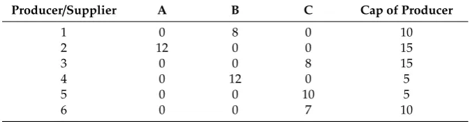
From vector 1, there are seven trucks, three suppliers, and six producers. Note that the values in the positions of all vectors are randomly generated. Trucks 1 to 7 have a capacity of 15, 12, 15, 15, 10, 12, and 15 tons, respectively. Demand for raw materials of all producers from the suppliers is shown in Table2(in tons).
Table 2.Raw material demand/capacity of producer (in tons).
Producer/Supplier A B C Cap of Producer
1 0 8 0 10
2 12 0 0 15
3 0 0 8 15
4 0 12 0 5
5 0 0 10 5
6 0 0 7 10
The DE code shown in Table1needed to be decoded so that the result of the proposed problem can be revealed. The decoding procedure was as shown in Algorithm 1.
materials from the supplier and the capacity of the producer can be seen in Table2. This information in Table3shows that the assignment was made.
Algorithm 1.Decoding Method
Input: supplier/producer vector; truck vector Output: proposed problem solution
Begin
Sort truck list in increasing values of position in vector (Tk)
Sort supplier/producer list in increasing order of value in position of supplier/producer vector (Lp) Whilepis less than the number of suppliers+number of producers
Assign truck (Tk) to supplier/producer according to their list (Lp) and create the supplier route as follows:
1. When the producer is being assigned, the closest supplier to that producer is selected to be in that route. 2. When the supplier is being assigned, the closest producer to that supplier is selected to be in that route. 3. The capacity of the truck must be considered so that it is not violated in the assignment.
p=p+1; end end
Table 3.Results of assignment of trucks to deliver raw material from the suppliers to the producers.
Truck Supplier Tons of Raw Material Carried Producerv Tons of Goods Carriedv
6 B 12 4 5
1 C 10 5 5
7 A 12 2 15
2 C 7 6 10
5 B 12 1 8
3 C 8 3 15
4.2. Performing the Mutation Process
Equation (10) was used to execute the mutation process. We assumed thatVm,n,G is a mutant vectormat positionnin iterationG.Xri,n,Gis the chosen target vectorrat positionnin iterationG.Fis the selected scaling factor.
Vm,n,G=Xr1,n,G+F(Xr2,n,G−Xr3,n,G) (10)
4.3. Performing the Recombination Procedure
WhenUm,n,Gis a trial vectormin positionnfor iterationG,CRis the selected parameter, which is normally set at a value of 0.6–0.9.Rnis randomly generated number. The trail vector generated from the recombination process can be executed using Equation (11):
Um,n,G={
Vm,n,Gr and Rn≤CR Xm,n,G otherwise
(11)
4.4. Performing the Selection Process
The selection process was used to reveal the next iteration target vector and was performed using Equation (12):
Xm,n,G+1=
Um,n,G if f(Um,n,G)≤ f(Xm,n,G)
Um,n,G if f(Um,n,G)≥ f(Xm,n,G)andRn ≤ Pag Xm,n,G otherwise
J. Open Innov. Technol. Mark. Complex.2019,5, 84 9 of 15
where f(Um,n,G)is the objective function of the trial vector, f(Xm,n,G)is the objective function of the current target vector,Rnis a random number, andPagis the probability of accepting the inferior solution, which can be calculated using Equations (13)–(16):
Pag= PF (13)
wherePFis the fixed probability of acceptance, which will be randomly generated and remains constant until the termination condition is met:
Pag=exp
−f(Um,n,G)−f(Xm,n,G)
TK (14)
whereTandKare predefined parameters;
Pag= 1− Cng
Max (15)
whereCngis the current iteration number andMaxis the maximum predefined number of iterations. The last equation is:
Pag=exp
−Cn
g
Max (16)
5. Computational Framework and Results
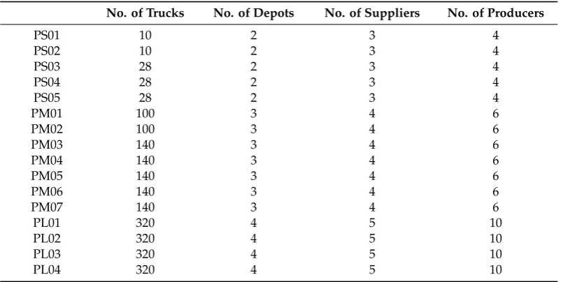
The algorithm was tested with 16 randomly generated datasets that have different numbers of depots, suppliers, and producers, as shown in Table4.
Table 4.Test instance details.
No. of Trucks No. of Depots No. of Suppliers No. of Producers
PS01 10 2 3 4
PS02 10 2 3 4
PS03 28 2 3 4
PS04 28 2 3 4
PS05 28 2 3 4
PM01 100 3 4 6
PM02 100 3 4 6
PM03 140 3 4 6
PM04 140 3 4 6
PM05 140 3 4 6
PM06 140 3 4 6
PM07 140 3 4 6
PL01 320 4 5 10
PL02 320 4 5 10
PL03 320 4 5 10
PL04 320 4 5 10
The test instances were divided into three groups: (1) small (PS01–PS05), (2) medium (PM01–PM07), and (3) large (PL01–PL04) groups of test instances. The number of iterations was used as the termination condition for all groups, set to 20,000, 40,000, and 100,000 iterations for small, medium, and large sizes of test instances, respectively.
Table 5.Details of proposed methods.
Name of Method AC Equation
DE-AC1 (13)
DE-AC2 (14)
DE-AC3 (15)
DE-AC4 (16)
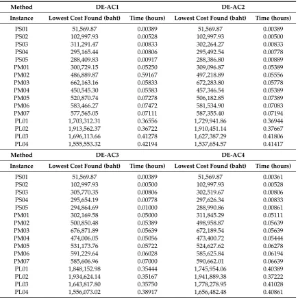
The results in Table6are the computation results of the experiment.
Table 6.Result of the experiment comparing the performance of the proposed heuristics.
Method DE-AC1 DE-AC2
Instance Lowest Cost Found (baht) Time (hours) Lowest Cost Found (baht) Time (hours)
PS01 51,569.87 0.00389 51,569.87 0.00389
PS02 102,997.93 0.00528 102,997.93 0.00500
PS03 311,291.47 0.00833 302,264.27 0.00833
PS04 295,165.44 0.00806 295,492.54 0.00778
PS05 288,409.83 0.00917 288,386.80 0.00889
PM01 300,729.15 0.05250 309,096.87 0.05389
PM02 486,889.87 0.59167 497,218.89 0.05556
PM03 662,163.16 0.05833 672,283.80 0.05778
PM04 450,545.30 0.05583 457,346.54 0.05389
PM05 520,870.74 0.07278 506,182.85 0.07389
PM06 583,466.27 0.07472 581,534.90 0.07083
PM07 577,565.05 0.07111 587,355.40 0.07194
PL01 1,703,312.31 0.36556 1,729,941.86 0.36944
PL02 1,913,562.37 0.36722 1,910,451.14 0.37667
PL03 1,696,113.66 0.41278 1,627,387.29 0.41806
PL04 1,555,553.32 0.42194 1,537,654.57 0.41417
Method DE-AC3 DE-AC4
Instance Lowest Cost Found (baht) Time (hours) Lowest Cost Found (baht) Time (hours)
PS01 51,569.87 0.00389 51,569.87 0.00361
PS02 102,997.93 0.00500 102,997.93 0.00528
PS03 305,770.35 0.00806 302,519.67 0.00806
PS04 295,654.19 0.00778 297,626.34 0.00833
PS05 294,864.69 0.01000 288,990.86 0.00861
PM01 302,169.58 0.05000 311,845.29 0.05111
PM02 500,850.48 0.05389 498,958.87 0.05639
PM03 676,871.89 0.05639 672,189.54 0.05639
PM04 474,006.05 0.05056 473,400.72 0.05444
PM05 531,173.76 0.05722 524,627.62 0.06278
PM06 591,229.64 0.06028 585,625.84 0.06194
PM07 585,606.96 0.07000 590,662.01 0.06639
PL01 1,848,152.98 0.35444 1,745,954.06 0.40389
PL02 1,934,624.14 0.35167 1,941,889.38 0.37222
PL03 1,643,817.80 0.35750 1,778,278.95 0.41028
PL04 1,556,073.02 0.38917 1,656,482.48 0.40861
J. Open Innov. Technol. Mark. Complex.2019,5, 84 11 of 15 J. Open Innov. Technol. Mark. Complex.2019, 5, x FOR PEER REVIEW 11 of 15
PM06 591,229.64 0.06028 585,625.84 0.06194 PM07 585,606.96 0.07000 590,662.01 0.06639 PL01 1,848,152.98 0.35444 1,745,954.06 0.40389 PL02 1,934,624.14 0.35167 1,941,889.38 0.37222 PL03 1,643,817.80 0.35750 1,778,278.95 0.41028 PL04 1,556,073.02 0.38917 1,656,482.48 0.40861
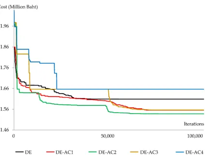
Figure 3. Best solution plot of the case study with 100,000 iterations.
From Figure 3, we can see DE-AC2 starts with one of the poorer solutions obtained from all proposed methods, but it is able to quickly find a better solution, and the solution always improved over time, which means that Equation (14) was very effective in terms of the required behaviors of the metaheuristics, diversification and intensification, while other equations provided diversification without intensification of the search, as was the case with DE and DE-AC1, or provided intensification but finally become stuck on a local optimum, as was the case for DE-AC3.
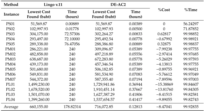
Then, we compared the proposed method with the optimal solution, or with the best solution that Lingo v.11 found within 240 h when the approach was not able to find the optimal solution. The outcomes of the problems are displayed in Table 7.
Table 7. Comparison of results of Lingo v.11 and DE-AC2.
Method Lingo v.11 DE-AC2
%Cost %Time
Instance Lowest Cost Found (baht)
Time (hours)
Lowest Cost Found (baht)
Time (hours)
PS01 51,569.87 0.00889 51,569.87 0.00389 0 56.24297 PS02 102,997.93 0.01778 102,997.93 0.00500 0 71.87852 PS03 304,175.00 72.57306 302,264.27 0.00833 0.62817 99.98852 PS04 293,497.00 72.10000 295,492.54 0.00778 −0.67992 99.98921 PS05 289,338.00 76.47056 288,386.80 0.00889 0.32875 99.98837
Figure 3.Best solution plot of the case study with 100,000 iterations.
From Figure3, we can see DE-AC2 starts with one of the poorer solutions obtained from all proposed methods, but it is able to quickly find a better solution, and the solution always improved over time, which means that Equation (14) was very effective in terms of the required behaviors of the metaheuristics, diversification and intensification, while other equations provided diversification without intensification of the search, as was the case with DE and DE-AC1, or provided intensification but finally become stuck on a local optimum, as was the case for DE-AC3.
Then, we compared the proposed method with the optimal solution, or with the best solution that Lingo v.11 found within 240 h when the approach was not able to find the optimal solution. The outcomes of the problems are displayed in Table7.
From the solution in Table7, we can see that DE could find an 8.47% different result than Lingo v.11, while it used 99.93% less computation time. A statistical test using the Wilcoxon sign rank test gave ap-value equal to 0.0917. This revealed that the proposed method and Lingo v.11 did not perform differently, which meant the proposed method could find the result just as effectively as Lingo v.11 while using 99.93% less computation time.
The traditional transportation plan was to plan the transportation every morning using the proposed methods without making any change when information was obtained. In this research, the traditional approach was changed by applying the idea of the taxi dispatching problem by reoptimizing the transportation plan when information from the factory was updated. We applied the traditional transportation planning method (traditional differential evolution (TDE)) and the one proposed in this paper (MDE) to PL01–PL04. The profits obtained from the TDE and MDE are shown in Table8. The percentage difference was calculated using Equation (17), wherePMDEis the profit generated by using MDE andPTDEis the profit generated using TDE.
%di f f = P
MDE−PTDE
Table 7.Comparison of results of Lingo v.11 and DE-AC2.
Method Lingo v.11 DE-AC2
%Cost %Time
Instance Lowest Cost Found (baht)
Time (hours)
Lowest Cost Found (baht)
Time (hours)
PS01 51,569.87 0.00889 51,569.87 0.00389 0 56.24297 PS02 102,997.93 0.01778 102,997.93 0.00500 0 71.87852 PS03 304,175.00 72.57306 302,264.27 0.00833 0.62817 99.98852 PS04 293,497.00 72.10000 295,492.54 0.00778 −0.67992 99.98921 PS05 289,338.00 76.47056 288,386.80 0.00889 0.32875 99.98837 PM01 286,221.00 240 309,096.87 0.05389 −7.99238 99.97755 PM02 482,858.00 240 497,218.89 0.05556 −2.97414 99.97685 PM03 638,687.00 240 672,283.80 0.05778 −5.26029 99.97593 PM04 439,173.00 240 457,346.54 0.05389 −4.13813 99.97755 PM05 501,680.00 240 506,182.85 0.07389 −0.89755 99.96921 PM06 549,831.00 240 581,534.90 0.07083 −5.76612 99.97049 PM07 544,372.00 240 587,355.40 0.07194 −7.89596 99.97003 PL01 1,499,230.00 240 1,729,941.86 0.36944 −15.38869 99.84607 PL02 1,678,520.00 240 1,910,451.14 0.37667 −13.81760 99.84305 PL03 1,501,070.00 240 1,627,387.29 0.41806 −8.41515 99.82581 PL04 1,399,260.00 240 1,537,654.57 0.41417 −9.89055 99.82743
Average 660,155.00 178.82314 716,072.85 0.12813 −8.47041 99.92835
Table 8.Comparison of results of the traditional differential evolution (TDE) and modified differential evolution (MDE).
Method TDE MDE (DE-AC2)
% Diff
Instance Daily Profit (baht) Daily Profit (baht)
PL01 4,145,871.00 4,425,178.00 6.31
PL02 4,389,594.00 4,664,836.00 5.90
PL03 4,241,879.00 4,528,747.00 6.33
PL04 4,581,436.00 4,895,536.00 6.42
From the computational results shown in Table8, we can see that IT was useful in the transportation planning process since it could increase a company’s profits by 5.9% to 6.42%.
6. Conclusions
We have presented a methodology to solve a vehicle dispatching problem. The case study involved planning to deliver raw materials to producers and take finished goods from the producers to the warehouse. When there was a signal indicating a need for raw materials from the company’s production planning software, trucks were dispatched from the distribution center immediately to pick up the products at the production plant or instructed to stop receiving the raw materials as the production plant requirements were filled. The decisions for routing the cargo were carried out continuously and more efficiently.
J. Open Innov. Technol. Mark. Complex.2019,5, 84 13 of 15
The transportation planning problem of the case study is a problem with multiple factors, including multiple producers, raw material sources, distribution centers, and types of truck. It is a basic fact that global shipping companies focus their attention and efforts on reducing transportation costs by having optimal transportation planning. The experiments indicated that the developed MDE obtained the exact solution according to all conditions or restrictions. It took an average of 0.12813 h to get the exact solution for the biggest problem. From the resulting analysis, it can be concluded that the solution from the proposed MDE was different from that of Lingo v.11 by 8.47% but took 99.93% less time.
Reducing the transportation cost meant the use of fuel was also reduced, which made for a lower impact in terms of global warming and other environmental concerns. Therefore, the proposed method not only reduces company costs but also generates sustainable transportation plans for the benefit of the company and the environment.
The new innovation we found here is the application of IT with the proposed heuristics, which is the modified different evolution algorithm. The proposed heuristics can support real-time decision-making and increase a company’s profits by up to 6.42%. This is a new innovation that can be applicable to many types of businesses.
Author Contributions: Methodology and software, N.S.; Conceptualization and resources, N.S. and R.A.; Writing—review and editing, R.A.
Funding:This project this funded by the Faculty of Engineering, Khonkean University, Thailand.
Acknowledgments:This paper was supported by KKU-En Grad Camp 2016, Faculty of Engineering, KhonKaen University, Thailand.
Conflicts of Interest:The authors declare no conflict of interest.
References
1. Kümmel, M.; Busch, F.; Wang, D.Z.W. Taxi Dispatching and Stable Marriage.Procedia Comput. Sci.2016,83, 163–170. [CrossRef]
2. An, S.; Zhang, X. Real-Time Hybrid In-Station Bus Dispatching Strategy Based on Mixed Integer Programming. Information2016,7, 43. [CrossRef]
3. Yu, J.; Zhou, X.; Zhao, H. Design and implementation of taxi calling and dispatching system based on GPS mobile phone. In Proceedings of the 4th International Conference on Computer Science & Education, Nanning, China, 25–28 July 2009. [CrossRef]
4. Chang, S.; Wu, C. Comparison of Environmental Benefits Between Satellite Scheduled Dispatching and Cruising Taxi Services. In Proceedings of the Transportation Research Board 89th Annual Meeting, Washington, DC, USA, 10–14 January 2010.
5. Bailey, W.A.; Clark, T.D. A simulation analysis of demand and fleet size effects on taxicab service rates. In Proceedings of the 19th Conference on Winter Simulation, Atlanta, GA, USA, 14–16 December 1987; pp. 838–844.
6. Pureza, V.; Laporte, G. Waiting and Buffering Strategies for the Dynamic Pickup and Delivery Problem with Time Windows.INFOR Inf. Syst. Oper. Res.2008,46, 165–176. [CrossRef]
7. Seow, K.T.; Sim, K.M. Collaborative assignment using belief-desire-intention agent modeling and negotiation with speedup strategies.Inf. Sci.2008,178, 1110–1132. [CrossRef]
8. Seow, K.T.; Lee, D.-H. Performance of Multiagent Taxi Dispatch on Extended-Runtime Taxi Availability: A Simulation Study.IEEE Trans. Intell. Transp. Syst.2010,11, 231–236. [CrossRef]
9. Kuhn, H.W. A tale of three eras: The discovery and rediscovery of the Hungarian Method.Eur. J. Oper. Res. 2012,219, 641–651. [CrossRef]
10. Zeng, T.; Hu, D.; Huang, G. The Transportation Mode Distribution of Multimodal Transportation in Automotive Logistics.Procedia Soc. Behav. Sci.2013,96, 405–417. [CrossRef]
11. Göçmen, E.; Erol, R. The Problem of Sustainable Intermodal Transportation: A Case Study of an International Logistics Company, Turkey.Sustainability2018,10, 4268. [CrossRef]
13. Aktel, A.; Yagmahan, B.; Özcan, T.; Yenisey, M.M.; Sansarcı, E. The comparison of the metaheuristic algorithms performances on airport gate assignment problem.Transp. Res. Procedia2017,22, 469–478. [CrossRef] 14. Fard, S.S.; Vahdani, B. Assignment and scheduling trucks in cross-docking system with energy consumption
consideration and trucks queuing.J. Clean. Prod.2019,213, 21–41. [CrossRef]
15. Guemri, O.; Nduwayo, P.; Todosijevi´c, R.; Hanafi, S.; Glover, F. Probabilistic Tabu Search for the Cross-Docking Assignment Problem.Eur. J. Oper. Res.2019,277, 875–885. [CrossRef]
16. Martins, S.; Ostermeier, M.; Amorim, P.; Hübner, A.; Almada-Lobo, B. Product-oriented time window assignment for a multi-compartment vehicle routing problem. Eur. J. Oper. Res. 2019,276, 893–909. [CrossRef]
17. Zhen, L.; Hu, Y.; Wang, S.; Laporte, G.; Wu, Y. Fleet deployment and demand fulfillment for container shipping liners.Transp. Res. Part B Methodol.2019,120, 15–32. [CrossRef]
18. Reihaneh, M.; Ghoniem, A. A branch-and-price algorithm for a vehicle routing with demand allocation problem.Eur. J. Oper. Res.2019,272, 523–538. [CrossRef]
19. Dukkanci, O.; Peker, M.; Kara, B.Y. Green hub location problem.Transp. Res. Part E Logist. Transp. Rev. 2019, 125, 116–139. [CrossRef]
20. Reyes, J.J.R.; Solano-Charris, E.L.; Montoya-Torres, J.R. The storage location assignment problem: A literature review.Int. J. Ind. Eng. Comput.2019,10, 199–224. [CrossRef]
21. Kaveh, A.; Vazirinia, Y. Construction Site Layout Planning Problem Using Metaheuristic Algorithms: A Comparative Study.Iran. J. Sci. Technol. Trans. Civ. Eng.2019,43, 105–115. [CrossRef]
22. Dantzig, G.; Ramser, J. The truck dispatching problem.Manag. Sci.1959,6, 80–91. [CrossRef]
23. Wang, S.; Tao, F.; Shi, Y.; Wen, H. Optimization of Vehicle Routing Problem with Time Windows for Cold Chain Logistics Based on Carbon Tax.Sustainability2017,9, 694. [CrossRef]
24. Mazzuco, D.E.; CarreirãoDanielli, A.M.; Oliveira, D.L.; Santos, P.P.P.; Pereira, M.M.; Coelho, L.C.; Frazzon, E.M. A concept for simulation-based optimization in Vehicle Routing Problems. IFAC-PapersOnLine2018,51, 1720–1725. [CrossRef]
25. Bettinelli, A.; Ceselli, A.; Righini, G. A branch-and-cut-and-price algorithm for the multi-depot heterogeneous vehicle routing problem with time windows.Transp. Res.2011,19, 723–740. [CrossRef]
26. Xu, Y.; Wang, L.; Yang, Y. A New Variable Neighborhood Search Algorithm for the Multi Depot Heterogeneous Vehicle Routing Problem with Time Windows.Electron. Notes Discret. Math.2012,39, 289–296. [CrossRef] 27. Dondo, R.G.; Cerda, J. A hybrid local improvement algorithm for large-scale multi-depot vehicle routing
problems with time windows.Comput. Chem. Eng.2009,33, 513–530. [CrossRef]
28. El-Sherbeny, N.A. Vehicle routing with time windows: An overview of exact, heuristic and metaheuristic methods.J. King Saud Univ. Sci.2010,22, 123–131. [CrossRef]
29. Beheshti, A.K.; Hejazi, S.R.; Alinaghian, M. The vehicle routing problem with multiple prioritized time windows:A case study.Comput. Ind. Eng.2015,90, 402–413. [CrossRef]
30. Bae, H.; Moon, I. Multi-depot vehicle routing problem with time windows considering delivery and installation vehicles.Appl. Math. Model.2016,40, 6536–6549. [CrossRef]
31. Afshar-Nadjafi, B.; Afshar-Nadjafi, A. A constructive heuristic for time-dependent multi-depot vehicle routing problem with time-windows and heterogeneous fleet.J. King Saud Univ. Eng. Sci.2017,29, 29–34. [CrossRef]
32. Baradaran, V.; Shafaei, A.; Hosseinian, A.H. Stochastic vehicle routing problem with heterogeneous vehicles and multiple prioritized time windows: Mathematical modeling and solution approach.Comput. Ind. Eng. 2019,131, 187–199. [CrossRef]
33. Hosny, M.I.; Mumford, C.L. Constructing initial solutions for the multiple vehicle pickup and delivery problem with time windows.J. King Saud Univ. Comput. Inf. Sci.2012,24, 59–69. [CrossRef]
34. Ahkamiraad, A.; Wang, Y. Capacitated and multiple cross-docked vehicle routing problem with pickup, delivery, and time windows.Comput. Ind. Eng.2018,119, 76–84. [CrossRef]
35. Soleimani, H.; Chaharlang, Y.; Ghaderi, H. Collection and distribution of returned-remanufactured products in a vehicle routing problem with pickup and delivery considering sustainable and green criteria.J. Clean. Prod.2018,172, 960–970. [CrossRef]
J. Open Innov. Technol. Mark. Complex.2019,5, 84 15 of 15
37. Wen, L.; Eglese, R.W. Minimum cost VRP with time-dependent speed data and congestion charge.Comput. Oper. Res.2015,56, 41–50. [CrossRef]
38. Poonthalir, G.; Nadarajan, R. A Fuel Efficient Green Vehicle Routing Problem with varying speed constraint (F-GVRP).Expert Syst. Appl.2018,100, 131–144. [CrossRef]
39. Alinaghian, M.; Naderipour, M. A novel comprehensive macroscopic model for time-dependent vehicle routing problem with multi-alternative graph to reduce fuel consumption: A case study.Comput. Ind. Eng. 2016,99, 210–222. [CrossRef]
40. Ghannadpour, S.F.; Zarrabi, A. Multi-objective heterogeneous vehicle routing and scheduling problem with energy minimizing.Swarm Evol. Comput.2019,44, 728–747. [CrossRef]
41. Praseeratasang, N.; Pitakaso, R.; Sethanan, K.; Kosacka-Olejnik, M.; Kaewman, S.; Theeraviriya, C. Adaptive Large Neighborhood Search to Solve Multi-Level Scheduling and Assignment Problems in Broiler Farms.J. Open Innov. Technol. Mark. Complex.2019,5, 37. [CrossRef]
42. Theeraviriya, C.; Pitakaso, R.; Sillapasa, K.; Kaewman, S. Location Decision Making and Transportation Route Planning Considering Fuel Consumption.J. Open Innov. Technol. Mark. Complex.2019,5, 27. [CrossRef] 43. Srivarapongse, T.; Pijitbanjong, P. Solving a Special Case of the Generalized Assignment Problem Using the
Modified Differential Evolution Algorithms: A Case Study in Sugarcane Harvesting.J. Open Innov. Technol. Mark. Complex.2019,5, 5. [CrossRef]
44. Praseeratasang, N.; Pitakaso, R.; Sethanan, K.; Kaewman, S.; Golinska-Dawson, P. Adaptive Large Neighborhood Search for a Production Planning Problem Arising in Pig Farming. J. Open Innov. Technol. Mark. Complex.2019,5, 26. [CrossRef]