CONTACT STRUCTURES ON OPEN 3-MANIFOLDS
James J. Tripp
A Dissertation
in
Mathematics
Presented to the Faculties of the University of Pennsylvania in Partial
Ful-fillment of the Requirements for the Degree of Doctor of Philosophy
2005
John B. Etnyre
Supervisor of Dissertation
David Harbater
Acknowledgments
Thank you to John Etnyre, my advisor, and Stephan Sch¨onenberger for many helpful
conversations and for reading drafts of this work. Also, thank you to Ko Honda, Will
Kazez, and Gordana Mati´c for their comments and questions during my talk at the
ABSTRACT
CONTACT STRUCTURES ON OPEN 3-MANIFOLDS
James J. Tripp
John B. Etnyre, Advisor
In this thesis, we study contact structures on any open 3-manifold V which is the interior of a compact3-manifold. To do this, we introduce proper contact isotopy invari-ants called the slope at infinity and the division number at infinity. We first prove several
classification theorems forT2×[0,∞),T2×R, andS1×R2using these concepts. This investigation yields infinitely many tight contact structures onT2×[0,∞),T2×R, and S1 ×R2 which admit no precompact embedding into another tight contact structure on the same space. Finally, we show that if everyS2 ⊂ V bounds a ball or anS2 end, then there are uncountably many tight contact structures on V that are not contactomorphic,
yet are isotopic. Similarly, there are uncountably many overtwisted contact structures on
Contents
1 Introduction and Statements of the Main Results 1
2 Background 6
2.1 Basic Contact Geometry . . . 6
2.2 Convex Surfaces . . . 10
2.2.1 Definitions and Basic Results . . . 10
2.2.2 Bypasses . . . 13
2.2.3 Convex Tori and the Farey Graph . . . 15
2.3 Known Classification Results . . . 17
2.3.1 Tight, Compact Contact Manifolds . . . 18
2.3.2 Tight, Open Contact Manifolds . . . 20
2.3.3 Overtwisted Contact Manifolds . . . 23
2.4 Taut Sutured Manifolds and Tight Contact Structures . . . 24
3.2 An Example . . . 29
4 Classification Theorems for Tight Toric Ends 32 4.1 Tight, minimally twisting toric ends with irrational slope at infinity . . . . 33
4.2 Tight, minimally twisting toric ends with rational slope at infinity . . . 37
4.3 Nonminimally twisting, tight toric ends . . . 44
4.4 Classifying Tight Contact Structures onS1×R2 andT2×R . . . 48
4.4.1 Factoring tight contact structures onS1×R2 . . . 48
4.4.2 Factoring tight contact structures onT2×R. . . 49
5 Proof of Theorem 1.0.2 and Theorem 1.0.3 51 5.1 Construction of the contact structures when∂M is connected . . . 56
5.2 Proof of Theorem 1.0.2 and Theorem 1.0.3 when∂M is connected . . . . 59
List of Figures
2.1 The Standard Contact Structure . . . 8
2.2 An Overtwisted Disk . . . 9
2.3 A Bypass . . . 13
2.4 Attaching a Bypass . . . 14
2.5 Characteristic Foliations of Tori . . . 16
2.6 The Farey Graph . . . 17
2.7 Bypass Attachment and the Farey Graph . . . 17
3.1 Perturbing a Torus to be Convex . . . 31
5.1 Special Curves on a Surface . . . 52
5.2 Sutures on the Boundary . . . 53
Chapter 1
Introduction and Statements of the
Main Results
Recently, there has been much work towards the classification of tight contact structures
on compact3-manifolds up to isotopy (relative to the boundary). In particular, Honda and Giroux provided several classification theorems for solid tori, toric annuli, torus bundles
over the circle, and circle bundles over surfaces [Gi1, Gi2, Gi3, Ho2, Ho3]. In
compar-ison, tight contact structures on open 3-manifolds have been virtually unstudied. Two main results dealing with open contact manifolds are due to Eliashberg. In [El1],
Eliash-berg shows that, in contrast to the situation forS2ends, there are uncountably many tight contact structures on S1 ×R2 that are not contactomorphic. The situation for closed 3-manifolds is different. Colin, Giroux, and Honda proved that an atoroidal 3-manifold
supports finitely many tight contact structures up to isotopy [CGH]. Honda, Kazez, and
Mati´c, and independently, Colin, show that an irreducible, toroidal 3-manifold supports countably infinitely many tight contact structures up to isotopy [HKM1, Co].
In this paper, we study tight contact structures on any open manifoldV that is the
interior of a compact manifold. Due to the failure of Gray’s Theorem on open contact
manifolds, we relegate ourselves to the study of tight contact structures up to proper
iso-topy, by which we mean isotopy of the underlying manifold rather than a one-parameter
family of contact structures. When we say that two contact structures are isotopic, we
will mean that they are connected by a one-parameter family of contact structures. We
first introduce two new proper isotopy invariants which we call the slope at infinity and
the division number at infinity of an endΣg×[0,∞)of an open contact manifold. These
invariants are most naturally defined for toric ends T2 ×[0,∞), where we take our in-spiration from the usual definition of the slope and division number of a convex torus.
Using these invariants and Honda’s work in [Ho2], we essentially classify tight contact
structures on toric endsT2×[0,∞). In particular, we show that there is a natural bijection between tight toric annuli and tight toric ends that attain the slope at infinity and have
finite division number at infinity. However, we also show that for any slope at infinity
therefore do not come from closed toric annuli. Interestingly, these contact structures are
strange enough that they cannot be properly embedded in another tight contact manifold.
This yields the following
Theorem 1.0.1. LetXbeT2×[0,1),T2×(0,1)orS1×D2, whereD2is the open unit
disk. LetX′ be another copy ofXparametrized asT2×[0,∞),T2×RorS1×R2. For
each slope at infinity, there exist infinitely many tight contact structures on X with that slope, distinct up to proper isotopy, which do not extend to a tight contact structure on
X′.
This result stands in contrast to Eliashberg’s original examples, all of which are
neigh-borhoods of a transverse curve in S3 and have a different slope at infinity. Using this embedding, it is easy to compactify his examples. Theorem 1.0.1 shows that, in general,
finding such a nice compactification is not straightforward.
Finally, just as high torus division number is a problem in the classification of toric
annuli, contact structures with infinite division number at infinity prove difficult to
un-derstand. However, we are able to use the notion of stable disk equivalence to partially
understand this situation. Precise statements of all of these results are in Section 4. In
Section 4.4, we use these results to reduce the classification of tight contact structures on
S1×R2 andT2×Rto the classification of the corresponding toric ends.
In the second half of the paper, we use the notion of the slope at infinity to prove a
generalization of Eliashberg’s result in [El3]:
connected 3-manifoldM with nonempty boundary such that every embedded S2 either
bounds a ball or is isotopic to a component of∂M. If∂M contains at least one compo-nent of nonzero genus, thenV supports uncountably many tight contact structures which are not contactomorphic, yet are isotopic.
Eliashberg’s proof involves computing the contact shape of the contact structures on
S1×R2, which in turn relies on a previous computation of the symplectic shape of certain subsets of Tn×Rn done in [Si]. We bypass the technical difficulties of computing the
symplectic shape by employing convex surface theory in the end ofV. The first step in
the proof is to put a tight contact structure on the manifold M with a certain dividing
curve configuration on the boundary. To do this, we use the correspondence between taut
sutured manifolds and tight contact structures covered in [HKM2]. We then find nested
sequences of surfaces which allow us to construct a contact manifold (V, ηs)for every
s ∈ (−2,−1). We distinguish these contact structures up to proper isotopy by showing
that they have different slopes at infinity. Since the mapping class group of an irreducible
3-manifold with boundary is countable (see [McC]), uncountably many of theηsare not
contactomorphic. To simplify the presentation of the proof, we first present the proof in
the case when ∂M is connected in Section 5.2. We deal with the case of disconnected
boundary in Section 5.3.
In [El1], Eliashberg declares a contact structures on an open3-manifoldV to be
tight at infinity. He then uses his classification for overtwisted contact structures in [El2]
to show that any two contact structures that are overtwisted at infinity and homotopic as
plane fields are properly isotopic. In contrast to this result, we have the following:
Theorem 1.0.3. Let V be any open 3-manifold which is the interior of a compact, connected 3-manifoldM with nonempty boundary such that every embedded S2 either
Chapter 2
Background
2.1
Basic Contact Geometry
In this section, we will summarize the most basic ideas and results in contact geometry
that will be necessary for our work. Many of these ideas have been summarized in a
more expanded form in survey articles and books. In particular, we refer the reader to
[Ho2] and [Et]. We have followed several sections in [Ho2] and [Et] very closely in our
exposition. We only consider contact geometry in dimension three, although many of the
basic concepts have analogs in higher dimensions. Unless otherwise specified,Mwill be
a3-manifold. We refer the reader to [He] for facts about3-manifolds.
atpfor everyp∈M, then we callξa contact structure and(M, ξ)a contact manifold. We now introduce three notions of equivalence of contact structures. Let (M1, ξ1) and(M2, ξ2)be two contact manifolds. We say that these contact manifolds are contact
diffeomorphic or contactomorphic if there is a diffeomorphism f: M1 → M2 such that f∗(ξ1) = ξ2. If theξi are on the same manifoldM, then we say that theξi are isotopic
if there is a family of contact structures ηt onM witht ∈ [0,1]such that η0 = ξ1 and
η1 =ξ2. We say that theξi are properly isotopic if there is a family of diffeomorphisms
φt of M such thatηt = φt∗(ξ1). One can use Moser’s Method, described in [Aeb], to
show that on a closed3-manifold, every isotopy is a proper isotopy. This is called Gray’s Theorem. Gray’s Theorem is not always true on open manifolds, since Moser’s Method
involves integrating a vectorfield.
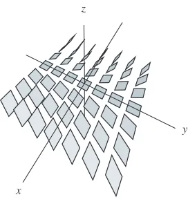
One of the ubiquitous examples of a contact structureξstdonR3is given as the kernel
to the globally defined form αstd = dz +xdy. This contact structure is shown in
Fig-ure 2.1. Note that this contact structFig-ure is vertically invariant. Another example onR3is given by the kernel of the formdz+r2dθ given in cylindrical coordinates.
Given that contact structures are inherently geometric objects, it makes sense to try
and understand them by trying to understand the curves and surfaces inside them. There
are two natural classes of curves: Legendrian and transverse curves. A curveγ inM is
Legendrian ifγis everywhere tangent toξand is transverse ifγis everywhere transverse to ξ. There is no natural dichotomy for surfaces inM. Algebraic manipulation of the
z
x
y
Figure 2.1: The contact structureker(dz+xdy).
there is no open subset of a surface Σ which integratesξ. This means that any surface Σ in a contact manifold has a singular, one-dimensional foliation defined atp ∈ M by TpΣ∩ξp. This singular foliation, denotedΣξ, is called the characteristic foliation ofΣ.
We say that two Legendrian (transverse) curvesγ1 andγ2 are Legendrian
(transver-sally) isotopic if there is an isotopy through embedded Legendrian (transverse) curves
that begins with γ1 and ends withγ2. One invariant of Legendrian curves up to
Legen-drian isotopy is the Thurston-Bennequin invariant. Let γ be a Legendrian curve inM,
Σ be a surface with ∂Σ = γ, and v be a vectorfield defined locally along γ which is
transverse to ξ. Let γ′ be the curve obtained by moving γ slightly along v. Define the
Thurston-Bennequin invariant ofγ, writtentb(γ), to be the signed intersection number of γ′ withΣ. We will give an easy way to compute this invariant after we introduce convex
surfaces.
We now discuss the local stability of a contact structure. The first result in this
Theorem 2.1.1. Let (M, ξ) be any contact 3-manifold and p ∈ M. Then there exist neighborhoods N of pin M, and U of the origin in R3 and a contact diffeomorphism
f: (N, ξ|N)→(R3, ξstd|U).
Darboux’s Theorem is a simple manifestation of the idea in contact geometry (proved
using Moser’s Method) that if two contact structures agree on some compact subset, then
they can be isotoped to agree on an open neighborhood of that subset. We now state the
most commonly used results which rely on this fact.
Theorem 2.1.2. Any two Legendrian (transverse) knots have contact diffeomorphic
neigh-borhoods.
Theorem 2.1.3. Let (Mi, ξi) be a contact manifold and Σi and embedded surface for
i = 0,1. If there is a diffeomorphism f: Σ0 → Σ1 that preserves the characteristic
foliation, then f can be extended to a contact diffeomorphism in some neighborhood of
Σ0.
Circle of tangencies
We now introduce a fundamental dichotomy in contact geometry. We say that a
con-tact manifold (M, ξ)is overtwisted if there exists a disk DinM, called an overtwisted
disk, with characteristic foliation as shown in Figure 2.2. We say that(M, ξ)is tight if it has no overtwisted disk.
2.2
Convex Surfaces
2.2.1
Definitions and Basic Results
As one might suspect, trying to prove anything using characteristic foliations can get quite
tricky. Therefore, we often work with surfaces which are embedded in a particularly nice
way with respect to the contact structure. A vectorfield v in a contact manifold(M, ξ) is called a contact vectorfield if the flow of the vectorfield is a one-parameter family of
contact diffeomorphisms. A surface ΣinM is convex if there is a contact vectorfieldv transverse to Σ. It turns out thatv need only be defined on a neighborhood ofΣ, since one can always write down an extension to a contact vectorfield defined on the whole
of M. Note that by definition a convex surface Σhas a natural product neighborhood structureΣ×(0,1)in which the contact structure is vertically invariant.
It turns out that convex surfaces are very easy to find. In fact, every surface isC∞
-close to a convex surface [Gi]. This is also true for a surface with Legendrian boundary,
as long as the twisting of the contact planes relative in the framing given by the surface
The important point about a convex surface is that we can distill all of the data about
the contact structure ξ in a neighborhood of the surface into a collection of curves on
the surface. We do this as follows. Let Σbe a convex surface and let v be the contact vectorfield transverse to Σ. Let Γ be the collection of pointsp ∈ Σwhere v(p) ⊂ ξp.
In [Gi], Giroux shows that this is generically a multi-curve, by which we mean a
one-dimensional submanifold ofΣ. Γalso satisfies the following conditions:
1. Σ\Γ = Σ+∪Σ−, whereΣ+andΣ−are disjoint subsurfaces.
2. Σξis transverse toΓ
3. There is a vectorfieldwand a volume formωonΣsuch that
(a) wdirectsΣξ in the sense that it is contained inΣξ and zero only whereΣξis
singular.
(b) the flow ofwexpandsωonΣ+and contractsωonΣ−.
(c) wpoints transversally out ofΣ+
We momentarily forget about the contact structure and just think about singular
one-dimensional foliations onΣ. We say that a multi-curveΓdivides a singular one-dimensional
foliationF onΣifF andΓsatisfy the above conditions, whereΣξis replaced byF. IfΓ
dividesF, then we callΓa collection of dividing curves. IfΣis a convex surface, then we denote the dividing curves corresponding toΣξ byΓΣ. The power of convex surfaces to
distill information about contact structures into the collection of dividing curves is based
Theorem 2.2.1 (Giroux Flexibility [Gi]). Suppose Fand Σξ are both divided by the
same multi-curveΓ.Then inside any neighborhoodN ofΣthere is an isotopyΦt: Σ→
N, t ∈[0,1]ofΣsuch that
1. Φ0 =inclusion ofΣintoN,
2. Φt(Σ)is a convex surface for allt,
3. Φtdoes not moveΓ,
4. (Φ1(Σ))ξ = Φ1(F).
This result is often referred to as Giroux Flexibility. A frequently used application of
Giroux Flexibility is the Legendrian Realization Principle.
Corollary 2.2.2 (Legendrian Realization Principle [Ka]). Let Σbe a convex surface andCbe a multicurve onΣ. AssumeC ⋔ΓΣandCis nonisolating, i.e., each connected
component ofΣ\Cnontrivially intersectsΓΣ. Then there is an isotopy (as in the Giroux Flexibility Theorem) such thatϕ1(C)is Legendrian.
When we say “LeRP”, we will mean “apply the Legendrian Realization Principle”
to a collection of curves. We will use this as a verb and call this process “LeRPing”
a collection of curves. It can be shown that for a Legendrian curve γ on Σ convex, tb(γ) =−1
2♯Γ∩γ.
We now state Giroux’s Criterion for determining whether or not a convex surface has
Theorem 2.2.3 (Giroux’s Criterion). LetΣbe a convex surface in(M, ξ). A vertically invariant neighborhood of Σ is tight if and only if Σ 6= S2 and ΓΣ contains no curves
that are contractible onΣorΣ = S2andΓΣ is connected.
2.2.2
Bypasses
Given a convex surface Σ, it is natural to ask what happens to the dividing set as we isotop the surface through the manifold. It turns out that the dividing set changes in a
“discrete” fashion, and the simplest change happens by attaching a bypass.
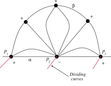
LetΣbe a convex surface andαbe a Legendrian arc inΣwhich intersectsΓΣin three points p1, p2, p3, wherep1 andp3 are endpoints ofα. A bypass is a convex half-diskD
with Legendrian boundary, where D∩Σ =α andtb(∂D) = −1. αis called the arc of
attachment of the bypass, andDis said to be a bypass alongαorΣ(Figure 2.3).
β Dividing curves α p p p 1 2 3 + + + + _ +
Figure 2.3: A bypass.
Each bypass carries a natural sign, so we say there are positive and negative bypasses.
the surface across the bypass.
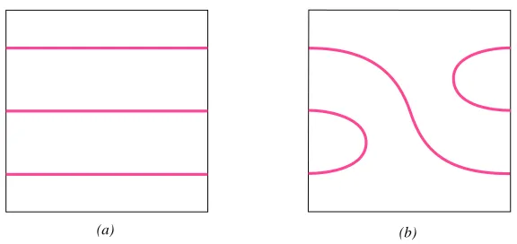
(a) (b)
Figure 2.4: The effect of attaching a bypass to a surfaceΣfrom the front to form a surface Σ′. The dividing setΓΣis (a) andΓΣ
′ is (b).
Finally, we describe a way of finding bypasses. This technique is known as the
Im-balance Principle and can be proved by using LeRP and Giroux Flexibility.
Theorem 2.2.4 (Imbalance Principle). Let S be a convex surface with Legendrian boundary.
1. If S = D2 so that tb(∂S) < −1, then there exists a bypass along∂S. Similarly,
ifS 6= D2,tb(∂S) ≤ −1, andΓ
S is boundary parallel, then there exists a bypass
along∂S.
2. LetS =S1×[0,1]. Iftb(S1× {1})< tb(S1× {0}), then there is a∂-parallel arc
2.2.3
Convex Tori and the Farey Graph
In this section, we discuss convex tori, our first example of a convex surface, and
explic-itly describe how bypass attachment changes the dividing set of the convex torus. The
dividing set of a convex torus must, first of all, be nonempty. This follows from some
facts about characteristic foliations which we will not go into here. By Giroux’s
Crite-rion, if the torus has any contractible dividing curves, then the ambient contact manifold
is overtwisted. If the torus is in a tight contact manifold, it cannot have any contractible
dividing curves. Therefore, the dividing set of a convex torus with no contractible
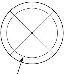
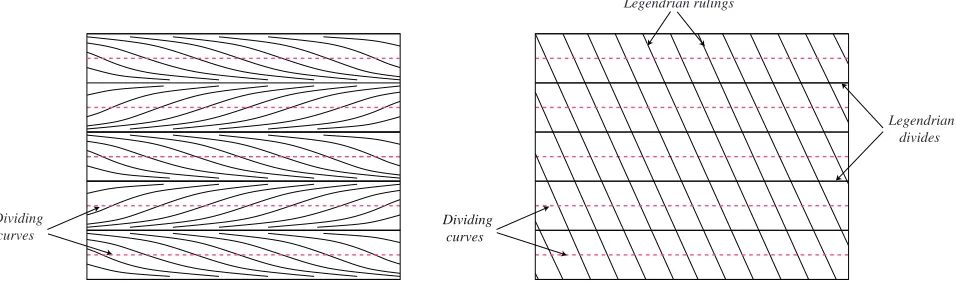
di-viding curves consists of an even number, 2n, of parallel curves, all having some slope s. We say that such a torus has slopes and division number n. Figure 2.5 shows two
convex tori. The right-hand side torus is said to be in standard form. We will often attach
bypasses along the curves labeled as Legendrian ruling cuves. Giroux Flexibility tells us
that we can always put a convex torus into standard form. Moreover, we can find ruling
curves of any rational slope that is different from the slope of the convex torus.
Suppose that the division number of a convex torus is greater than1. If we attach a bypass along a ruling curve, then one can check that the division number goes down by
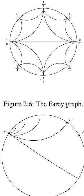
one. If the division number is1, then we can keep track of the change in slope by using the Farey graph (Figure 2.6). The Farey graph can be described as follows: The set of
vertices of the Farey graph is Q∪ {∞}on ∂H. (More precisely, fix a fractional linear transformation f from the upper half-plane model of hyperbolic space to the unit disk
Dividing curves
Dividing curves
Legendrian rulings
Legendrian divides
Figure 2.5: The left-hand side is a torus with nonsingular, Morse-Smale characteristic
foliation. The right-hand side is a torus in standard form. Here the sides are identified
and the top and bottom are identified.
edge between pq and pq′′ if and only if the corresponding shortest integer vectors form an
integral basis forZ2. (The edge is usually taken to be a geodesic inH.) The usefulness of the Farey graph is contained in the following result which is due to Honda.
Theorem 2.2.5 (Honda [Ho2]). Let s = slope(ΓT2). If a bypass is attached along a
closed Legendrian ruling curve of slope s′, then the slope s′′ on the resulting convex surface is obtained as follows: Let[s′, s)⊂ ∂Hbe the counterclockwise interval froms′ tos. Thens′′is the point on[s′, s)which is closest tos′and has an edge tos.
1 0 _ 1 _ 0 1 _ 2 1 _ 1 2 _ 1 1 _ -2 1 _
- - 1
2
_
1
Figure 2.6: The Farey graph.
s s'
s''
Figure 2.7: Bypass attachment using the Farey graph.
2.3
Known Classification Results
In this section, we will outline the basic classification results in contact geometry for
closed manifolds and highlight the ones which we will build upon later. We group these
results into theorems concerning classification of tight contact structures and theorems
2.3.1
Tight, Compact Contact Manifolds
The result which gets most any classification theorem off the ground is Eliashberg’s
The-orem [El4].
Theorem 2.3.1 (Eliashberg [El4]). Fix a characteristic foliation F adapted toΓ∂B3 =
S1. Then there is a unique tight contact structure onB3up to isotopy relative to∂B3. Much of the progress towards classifying tight contact structures on compact
mani-folds is due to the development of convex surface theory, the usefulness of which is due
to Eliashberg’s result. In general, the scheme for determining an upper bound on the
number of tight contact structures on a Haken 3-manifold (a Haken3-manifold can be cut up along successive surfaces until all one is left with are balls) up to isotopy is as
follows: Make each successive cutting surface convex and cut along it, keeping track of
the dividing set. Then, once you are left with balls, you invoke the result of Eliashberg,
and then examine all possible dividing sets on the cutting surfaces as you glue them back
together.
We will now proceed to classification results forT2×I. We first identify the most basic building block for a contact structure on this space: the basic slice. ConsiderT2× [0,1]with convex boundary conditions #Γ0 = #Γ1 = 2, s0 = ∞, and s1 = 0. Here
we write Γi = ΓT2×{i} andsi = slope(Γi). (Using a diffeomorphism of T2 ×I, there
is an analogous result when the shortest integer vectors corresponding to s0 ands1form
to T2 × {i}has slope(Γ
T′)in the interval(0,+∞)). These T2 ×[0,1]layers are basic
slices. These two tight contact structures are formed by attaching a bypass along a ruling
curve of slope 0, so each has a sign which depends on the sign of the bypass that is attached. We call a basic slice positive (negative) basic slice if it is formed by attaching
a positive (negative) bypass.
Given any tight, minimally twisting contact structure onT2×Iwith convex boundary, each component of which has division number1, one can act by an element of SL2(Z) so that the slope ofT2× {0}is−1and the slope ofT2× {1}is−p
q. We now write− p q
using the continued fraction expansion
−pq =r0− 1 r1− 1
r2···−1 rk
,
whereri ≤ −2. We will abbreviate this continue fraction expansion as(r0, r1, . . . , rk−1, rk).
LetAbe a convex annulus with boundary on ruling curves of slope0on opposite bound-ary components. By the Imbalance Principle, there is a bypass along T2 × {1}. We attach this bypass. After bypass attachment, we obtain a convex torus T′ isotopic toT,
such that T andT′ cobound aT2 ×I. Denoteslope(Γ
T′) = −p ′
q′. One can prove that,
in fact, −pq′′ has continued fraction expansion(r0, r1, . . . , rk−1, rk+ 1). In terms of the
Farey graph, we have moved counterclockwise. We successively peel off T2 ×I layers according to the Farey tessellation. The sequence of slopes is given by the continued
fraction expansion, or, equivalently, by the shortest sequence of counterclockwise arcs in
We group the basic slices into continued fraction blocks. Each block consists of all the
slopes whose continued fraction representations are of the same length. It turns out that
we may shuffle basic slices which are in the same continued fraction block. This, along
with some work from [Ho2] that we suppress for brevity, means that the contact structure
in a continued fraction block depends only on the number of positive (or negative) basic
slices in a continued fraction block. Keeping careful track of the continued fraction
expansion together with what we have said, implies
Theorem 2.3.2 (Honda [Ho2]). Let ΓTi, i = 0,1, satisfy #ΓTi = 2 and s0 = −1,
s1 = −pq, where p > q > 0. Then the number of tight contact structures with these boundary conditions, up to isotopy relative to the boundary, is equal to |(r0 + 1)(r1 + 1)· · ·(rk−1+ 1)(rk)|.
The main point to take away from this Theorem is that the isotopy classification of
tight contact structures on T2 ×I boils down to counting the number of positive basic slices in each continued fraction block. This, together with the boundary conditions,
determines the contact structure up to isotopy relative to the boundary. For the case of
nonminimally twisting, tight contact structures, we refer the reader to [Ho2].
2.3.2
Tight, Open Contact Manifolds
Before beginning to discuss tight, open contact manifolds, we should say something
about the equivalence relation up to which we are classifying the contact structures. We
many cases uninteresting. For example, consider S1×R2. Given any contact structure on this space, one can always find a transverse knot in the same isotopy class asS1×{0}. Since all transverse knots are locally the same, all contact structures on S1 × R2 are isotopic. It is therefore more reasonable to classify contact structures up to proper isotopy,
which, as we shall see, is a more interesting equivalence relation.
In [El1], Eliashberg proves that the proper isotopy classification of contact structures
onR3 coincides with the isotopy classification of contact structures onS3. In particular, this means that there is a unique tight contact structure onR3and the overtwisted contact structures are countable. Eliashberg’s proof essentially shows the following:
Theorem 2.3.3 (Eliashberg). LetF be a foliation onS2×{0}with a tight neighborhood.
ThenS2×[0,∞)has a unique tight contact structureξwithS2× {0}
ξ =F.
This means that when looking at contact structures on open manifolds withS2 ends, one can essentially ignore the contact structure in theS2 end.
The first result for a manifold other that S2 × [0,∞) is Eliahsberg’s existence re-sult for S1 ×R2 [El3]. These contact manifolds are all found as open subsets of S3 with the unique, tight contact structure given by the1-formα = ρ2
1dφ1 +ρ22dφ2, where (ρ1eiφ1
, ρ2eiφ2
) are the standard complex coordinates from C2 restricted to S3. For a positiveδ <1, letUδ ={(z1, z2)|ρ1 < δ}, an open torus inS3.
Theorem 2.3.4 (Eliashberg [El3]). Uδ is contact diffeomorphic toUδ′ if and only if the
difference δ12 −
1
One direction is fairly straightforward. Ifδ12 −
1
δ′ =−kwithka positive integer, then
the map(ρ1, φ1, φ2)→(√ρ1
1+kρ2 1
, φ1−kφ2, φ2)is contact and sendsUδ ontoUδ′.
The reverse direction is not nearly as straightforward. Eliashberg’s proof relies on
an invariant of a contact manifold V2n−1 called the contact shape, which is a subset H1(V;R) and is computed with respect to a manifold Mn. One computes the contact
shape by looking at the symplectization of the contact manifold and computing the
sym-plectic shape with respect toM. The symplectic shape of an exact, symplectic manifold (X, ω =dλ)with respect toM and a mapα: H1(X;R)→H1(M;R)is the collection off∗(λ)∈H1(M;R)wheref: M ֒→X is an embedding such thatf∗ =α.
Eliashberg derives the formulaic relationship betweenδandδ′by computing the
con-tact shape of the open region inΓδ,δ′ = Uδ\Uδ′ (assuming δ > δ′) with respect toT2.
To do this, he embeds Γδ,δ′ inside T2 ×S1, the unit cotangent bundle of T2. He then
relies on a computation of Sikorav [Si] about the symplectic shape of open subsets of
the cotangent bundle of Tn which have the formTn×A, where A ⊂ Rn is open (the
symplectization of the embedding of Γδ,δ′ has this form). Thek in the statement of the
theorem is the number of Dehn twists the contact diffeomorphism performs about the
meridinal disks inUδ and shows up when inducing maps on the level of cohomology.
We mention these techniques to contrast the methods in this thesis. While the contact
shape is in the same circle of ideas as Gromov’s result about intersections of exact
La-grangian manifolds [Gr], our main tool will be convex surface theory, which is of a very
2.3.3
Overtwisted Contact Manifolds
We now turn our attention to overtwisted contact structures. The most fundamental result
in this area is Eliashberg’s classification of overtwisted contact structures:
Theorem 2.3.5 (Eliashberg [El2]). Classification of overtwisted contact structures on a
closed manifoldM up to isotopy coincides with the homotopical classification of plane fields. If∂M 6=∅, then isotopy and homotopy are fixed in a neighborhood of∂M.
On an open manifold V, an overtwisted contact structure can be tight at infinity or
overtwisted at infinity. An overtwisted contact structure is tight at infinity if there exists
a compact set K ⊂ V such that V \K is tight. Analogously, an overtwisted contact
structure is overtwisted at infinity if for every compact setK ⊂V the manifoldV \Kis
overtwisted. These notions were introduced by Eliashberg [El1] so that he could prove a
similar theorem for open manifolds.
Theorem 2.3.6 (Eliashberg [El1]). Letξ1 andξ2 be two contact structures overtwisted at infinity on an open3-manifoldM. Ifξ1 andξ2 are homotopic as plane fields, then they are properly isotopic.
The proof of this result is essentially a repeated application of Eliahsberg’s homotopy
classification of overtwisted contact structures on compact manifolds. We now sketch
the proof. Begin with and exhaustion U1 ⊂ U2 ⊂ · · · ⊂ M of M by open domains
contact structureτ onV as follows: setτ =ξ1onU1; for eachi,τ coincides withξ2 near ∂U2iand withξ1near∂U2i+1;τis homotopic relative to the boundary toξ1(ξ2) onU2i+1\ U2i−1 (U2i\U2i−2);τ is overtwisted onUi+1\Ui. According to Eliashberg’s homotopy
classification of overtwisted contact structures, there is an isotopy on U2i \U2i−2 fixed near the boundary takingτtoξ2. Similarly, there is an isotopy onU2i+1\U2i−1fixed near the boundary fromτ toξ1. Hence, we have inductively constructed a proper isotopy on
V fromτ to eitherξi. Clearly, such a proof will not work for manifolds that are tight at
infinity, since we cannot construct an exhaustion that satisfies the desired properties.
2.4
Taut Sutured Manifolds and Tight Contact
Struc-tures
For the reader’s convenience, we list some of the definitions and results in [HKM2] which
we will need later. A sutured manifold(M, γ)is a compact oriented3-manifoldM to-gether with a set γ ⊂ ∂M of pairwise disjoint annuli A(γ) and tori T(γ). R(γ) de-notes ∂M \int(γ). Each component ofR(γ)is oriented. R+(γ)is defined to be those components of R(γ)whose normal vectors point out of M and R−(γ) is defined to be
R(γ)\R+(γ). Each component ofA(γ)contains a suture which is a homologically
non-trivial, oriented simple closed curve. The set of sutures is denoteds(γ). The orientation
on R+(γ), R−(γ), and s(γ)are related as follows. If α ⊂ ∂M is an oriented arc with
must start inR+(γ)and end inR−(γ).
A sutured manifold with annular sutures is a sutured manifold(M, γ)such that∂M is nonempty, every component ofγ is an annulus, and each component of∂M contains a
suture. A sutured manifold(M, γ)with annular sutures determines an associated convex
structure(M,Γ), whereΓ =s(γ). For more on this correspondence, see [HKM2]. A transversely oriented codimension-1foliationF is carried by(M, γ)ifF is
trans-verse to γ and tangent toR(γ)with the normal direction pointing outward alongR+(γ) and inward along R−(γ), andF|γ has no Reeb components. F is taut if each leaf
in-tersects some closed curve or properly embedded arc connectingR−(γ)toR+(γ)
trans-versely.
LetS be a compact oriented surface with components S1, . . . , Sn. Letχ(Si)be the
Euler characteristic ofSi. The Thurston norm ofS is defined to be
x(S) = X
χ(Si)<0
|χ(Si)|.
A sutured manifold(M, γ)is taut if
1. M is irreducible.
2. R(γ)is Thurston norm minimizing inH2(M, γ); that is, ifSis any other properly
embedded surface with[S] = [R(γ)], thenx(R(γ))≤x(S).
3. R(γ)is incompressible inM.
Theorem 2.4.1. A sutured manifold(M, γ)is taut if and only if it carries a transversely oriented, taut, codimension-1foliationF.
We require the following result due to Honda, Kazez, and Mati´c [HKM2].
Theorem 2.4.2. Let(M, γ)be an irreducible sutured manifold with annular sutures, and let(M,Γ)be the associated convex structure. The following are equivalent.
1. (M, γ)is taut.
2. (M, γ)carries a taut foliation.
Chapter 3
The End of an Open Contact Manifold
and Some Invariants
3.1
Definitions of the Invariants
Let (V, ξ)be any open contact 3-manifold that is the interior of a compact 3-manifold M such that ∂M is nonempty and contains at least one component of nonzero genus.
Fix an embedding of V ֒→ int(M)so that we can think of V as M \∂M. Choose a boundary componentS ⊂ ∂M and letΣ ⊂ M \∂M be an embedded surface isotopic toS inM. Note thatS andΣbound a contact manifold(Σ×(0,1), ξ). We call such a manifold, along with the embedding intoV, a contact end corresponding toS andξ. Let
Ends(V, ξ;S)be the collection of contact ends corresponding toS andξ.
closed curve which bounds a punctured torusT inS. Fix a basisB of the first homology
ofT. LetΣ⊂ V be a convex surface which is isotopic toS inM and contains a simple closed curveγwith the following properties:
1. γ is isotopic toλonΣ, where we have identifiedΣandSby an isotopy inM.
2. γ intersectsΓΣtransversely in exactly two points.
3. γ has minimal geometric intersection number withΓΣ.
Call any such surface well-behaved with respect toS andλ. Note that there exists a
simple closed curveµ⊂ΓΣ which is contained entirely inT. Let the slope ofΣ, written slope(Σ), be the slope ofµmeasured with respect to the basis B of the first homology
ofT. WhenSis a torus, we omit all reference to the curveλas it is unnecessary for our
definition.
LetE ∈ Ends(V, ξ;S). LetC(E)be the set of all well-behaved convex surfaces in the contact endE. IfC(E)6=∅, then define the slope ofE, to be
slope(E) = sup Σ∈C(E)
(slope(Σ)).
that this slope is attained if for each E ∈ Ends(V, ξ;S)there exists a Σ ∈ C(E)with that slope. Note that any slope that is attained must necessarily be rational.
LetΣ∈ C(E). Define the division number ofΣ, writtendiv(Σ)to be half the number of dividing curves and arcs on T. When Σ is a torus, this is the usual torus division number. IfC(E)6=∅, then let
div(E) = min
Σ∈C(E)(div(Σ)).
Note thatdiv: Ends(V, ξ, S)→N∪ {∞}is a net, where we endowN∪ {∞}with the discrete topology. If C(E) is nonempty for a cofinal sequence of contact ends, then we call the limit the division number at infinity of (V, ξ;S, λ, B)or the division number at
infinity of (V, ξ)ifS, λ, and B are understood from the context. Note that the slope at infinity and the division number at infinity are proper isotopy invariants.
3.2
An Example
In this section, we compute the slope and infinity and the division number at infinity for
Eliashberg’s examples of uncountably many open, solid tori that are not contact
diffeo-morphic. We will show that the Uδ are, in fact, distinct up to proper isotopy. First, we
examine∂Uδ. Note that there are natural coordinates onT2 given by φ1 andφ2. These
coordinates induce coordinates on the homology of∂Uδ. In these coordinates, the
char-acteristic foliation of∂Uδ is linear and has slopeδ2/(δ2−1). We call a torus with linear
Uδ isδ2/(δ2−1)and the division number at infinity is1.
To compute the slope at infinity, we must have several facts at our disposal. First,
every T2 ×I inS3 with the standard tight contact structure is minimally twisting. This fact follows from the fact thatT2×{0}must bound a solid torusSwhich does not contain the T2× {1}. IfT2 ×I we not minimally twisting, then we could find an overtwisted meridinal disk insideS∪T2×I.
The second fact is the following: Given a pre-Lagrangian torusT ⊂S3with rational slopesand an open neighborhoodNofT, one can perturbT to be a convex torusT′ ⊂N
such thatslope(T′) =sanddiv(T′) = 1. To prove this, first recall that the characteristic
foliation onT determines the contact structure in a neighborhood ofT. We construct the
standard model for this neighborhood as follows: ConsiderR3with the contact structure ξ = ker(dz +xdy). If we quotient R3 by z 7→ z + 1 and y 7→ y + 1, we will get M = R× T2. Since the contact structure is preserved by this action, ξ will induce a contact structure on M. Clearly, there exists a diffeomorphism taking T to {0} × T2 that preserves the characteristic foliations. Therefore, they have contact diffeomorphic
neighborhoods. Now, perturb{0} ×T2intoΣ = {(f(z), y, z)}viaf, the graph of which is shown in Figure 3.1. The resulting torus Σ will be convex and have characteristic foliation identical to the torus on the left-hand side of Figure 2.5.
Given these facts, the computation of the slope at infinity is fairly straightforward.
Note that, given any neighborhood N of ∂Uδ,we can find pre-Lagrangian tori inside
z f ( z )
Figure 3.1: The graph off.
of these tori to be convex. Choose a sequenceTiof such convex tori with division number
1and slopes converging toδ2/(δ2−1). To show that the slope at infinity is well-defined in this case (and therefore that our sequence actually computes the slope at infinity), assume
that there is another sequence of convex toriSi that leave every compact set ofUδ, have
division number1, and have slopes converging to some numberrother thanδ2/(δ2−1). By the minimal twisting condition,r < δ2/(δ2−1). Letǫ=δ2/(δ2−1)−r. There exists an msuch|slope(Tm)−δ2/(δ2−1)| ≤ ǫ/4and ann such that|slope(Sn)−r| ≤ ǫ/4
and Sn lies outside of the compact set bounded by Tn insideUδ. But, the existence of
Tm andSn violates minimal twisting, sinceSn lies outside of the compact set bounded
byTninsideUδ. Hence, theSi do not exist, so the slope at infinity is well-defined and is
equal toδ2/(δ2−1). Given the existence of the family of toriT
i, we see that the division
Chapter 4
Classification Theorems for Tight Toric
Ends
In this section, we study tight contact structures on toric ends. We say that a toric end is
minimally twisting if it contains only minimally twisting toric annuli. We first show that
it is possible to refer to the slope at infinity and the division number at infinity for toric
ends.
Proposition 4.0.1. Let T2 ×[0,∞) be a tight toric end. Then the division number at
infinity and the slope at infinity are defined.
Proof. First note thatC(E)is nonempty for any endEsince the condition for being well-behaved is vacuously true for tori. Also, note that the division number at infinity exists
by definition.
at infinity is ∞. Otherwise, there exists an end E = T2 ×[0,∞)such that for no end F ⊂ E is slope(F) = ∞. This means that E is minimally twisting. Without loss of generality, assumeTi =T2×iis convex with slopesi. Note that thesiform a clockwise
sequence on the Farey graph and are contained in a half-open arc which does not contain
∞. Sinceslope(F)≤sifor any endF ⊂T2×[i,∞), our net is convergent, so the slope
at infinity is defined.
4.1
Tight, minimally twisting toric ends with irrational
slope at infinity
In this section, we study tight, minimally twisting toric ends (T2 ×[0,∞), ξ) with
ir-rational slope r at infinity and with convex boundary satisfying div(T2 ×0) = 1 and slope(T2×0) =−1. Unless otherwise specified, all toric ends will be of this type.
We first show how to associate to any such toric end a functionfξ: N → N∪ {0}.
There exists a sequence of rational numbers qi on the Farey graph which satisfies the
following:
1. q1 =−1and theqi proceed in a clockwise fashion on the Farey graph.
2. qi is connected toqi+1by an arc of the graph. 3. Theqi converge tor.
graph unlessj is adjacent toi.
We can form this sequence inductively by takingq2 to be the rational number which
is closest to r on the clockwise arc of the Farey graph [−1, r] between −1 and r and has an edge of the graph from −1 to q2. Similarly, construct the remaining qi. Any
such sequence can be grouped into continued fraction blocks. We say that qi, . . . , qj
form a continued fraction block if there is an element ofSL2(Z)taking the sequence to
−1, . . . ,−m. We callmthe length of the continued fraction block. We say that this block
is maximal if it cannot be extended to a longer continued fraction block in the sequence
qi. Sinceris irrational, maximal continued fraction blocks exist. Denote these blocks by
Bi. To apply this to our situation, we need the following.
Proposition 4.1.1. There exists a nested sequence of convex tori Ti with div(Ti) = 1
such thatslope(Ti) = qi. Moreover, any such sequence must leave every compact set.
Proof. By the definition of slope at infinity, for anyǫ, there is an endEsuch thatslope(E) is within ǫofr. This means that there is a convex torus T inE with slope lying within
2ǫ of r. Note that since our toric end is minimally twisting and has sloper at infinity, slope(T) ∈ [−1, r). We attach bypasses to T so that div(T) = 1. The toric annulus bounded byT2×0andT contains the toriT
iwithqi lying couterclockwise toslope(T).
Fix these first Ti. Choose another torus T′ outside of the toric annulus with slope even
closer to r. Again, adjust the division number of T′ so that it is1 and factor the toric
annulus bounded byT andT′to find another finite number of ourT
i. Proceeding in this
compact set by the definition of the slope at infinity. For, if not, then we could find a torus
T in any end withslope(T)> r, which would show that the slope at infinity is notr.
This factors the toric end according to our sequence of rationals. We say that a
con-secutive sequence ofTiform a continued fraction block if the corresponding sequence of
rationals do. Each maximal continued fraction blockBidetermines a maximal continued
fraction block of tori which we also callBi. We think ofBias a toric annulus.
To each continued fraction block, we letnj be the number of positive basic slices in
the factorization of Bi byTj. Define fξ: N → N∪ {0} byfξ(j) = nj. To show that
the functionfξis independent of the factorization byTi, supposeTi′ is another
factoriza-tion with the same properties asTi. LetBj′ denote the corresponding continued fraction
blocks. Fixj. There existsn large such that the toric annulusAbounded byTn andT1
contains the continued fraction blocks Bj andB′j. Extend the partial factorization ofA
byB′
j. Recall that one can compute the relative Euler class via such a factorization and
that it depends on the number of positive basic slices in each continued fraction block
[Ho2]. Therefore,Bj andBj′ must have the same number of positive basic slices.
Given an irrational numberr, letF(r) denote the collection of functions f: N → N∪ {0}such thatf(i)does not exceed one less than the length ofBi. We can now state
a complete classification of the toric ends under consideration.
Theorem 4.1.2. Let(T2×[0,∞), ξ)be a tight, minimally twisting toric end with convex
boundary satisfyingdiv(T2×0) = 1andslope(T2×0) = −1. Suppose that the slope
fξ: N→N∪{0}which is a complete proper isotopy (relative to the boundary) invariant.
Moreover, given anyf ∈ F(r), there exists a toric end(T2×[0,∞), ξ)such thatf
ξ =f.
Proof. If fξ = fξ′, then we can shuffle bypasses within any given continued fraction
block so that all positive basic slices occur at the beginning of the block. Since the
number of positive basic slices in any continued fraction block is the same, it is clear that
they are properly isotopic.
It is a straightforward application of the gluing theorem for basic slices in [Ho2] to
show that we can construct a toric annulus corresponding to the desired continued fraction
blocks. The fact that they stay tight under gluing follows from the fact that overtwisted
disks are compact.
Corollary 4.1.3. Let (T2 ×[0,1), ξ)be a tight, minimally twisting toric end with
irra-tional sloperat infinity. Supposefξ(i)is not maximal or minimal for an infinite number
of numbers i. Then there does not exist any tight, toric end (T2 ×[0,∞), η)such that ξ|T2×[0,1) =η|T2×[0,1).
Proof. Assume that there were an inclusionφ: (T2×[0,1), ξ)→(T2×[0,∞), η). Per-turb T2 × {2} to be convex of slope b. Choose a convex torus φ(T′) of slope a. As
before, we have a minimal, clockwise sequence of rationals qj for 1 ≤ j ≤ n on the
Farey graph such that q1 = a, qn = b, and qi is joined to qi+1 by an arc of the graph. Let qm be the rational closest to q1 such that r lies clockwise to q1 and
counterclock-wise to qm. By our assumption on fξ, there exists a continued fraction block of tori
Tj1, . . . , Tjk ⊂ (T
Moreover, we can assume that the corresponding sequence of rationals lies clockwise
to qm−1 and counterclockwise to qm. Perturb tori Tin and Tout in (T2 × [0,∞), η) to
be convex of slopesqm−1 andqm, respectively, such that the basic slice bounded byTin
and Tout contains φ(Tj1), . . . , φ(Tjk). This is a contradiction, since a basic slice
can-not be formed by gluing basic slices of opposite signs unless the contact structure η is
overtwisted [Ho2].
4.2
Tight, minimally twisting toric ends with rational slope
at infinity
We now consider tight, minimally twisting toric ends(T2×[0,∞), ξ)with rational slope rat infinity and with convex boundary satisfyingdiv(T2×0) = 1andslope(T2×0) =
−1. Unless otherwise specified, all toric ends will be of this type. We first deal with the
situation when the slope at infinity is not attained.
We show how to every toric end under consideration we can assign a function
fξ: {1, . . . , n(r)} × {1,−1} →N∪ {0,∞}.
We proceed in a fashion similar to the irrational case. Given r rational, there exists a
sequence of rationalsqi satisfying the following:
1. q1 =−1and theqi proceed in a clockwise fashion on the Farey graph.
3. Theqi converge tor, butqi 6=rfor anyi.
4. The sequence is minimal in the sense thatqiandqj are not joined by an arc of the
tesselation unlessj is adjacent toi.
We construct such a sequence inductively just as in the irrational case, except we
never allow the rationals qi to reach r. Note that such a sequence breaks up naturally
into n−1finite continued fraction blocksBi and one infinite continued fraction block
Bn(i.e.,Bncan be taken to the negative integers after action bySL2(Z)). Note thatnis
completely determined by r. Just as in the irrational case, there exist nested covex tori
Ti withdiv(Ti) = 1andslope(Ti) = qi. We can argue as in the irrational case to show
that these tori must leave every compact set of the toric end. We will also refer to the
collection of toriTicorresponding toBi by the same name.
We will now constructfξ. Let fξ(i,±1)be the number of positive (negative) basic
slices in the continued fraction blockBi. Of course, for a finite continued fraction block,
fξ(i,1)determinesfξ(i,−1). However, this is clearly not the case forBn.
As in the irrational case, letF(r)be the collection of functionsf: {1, . . . , n(r)} ×
{1,−1} → N∪ {0,∞}such thatfξ(i,1) +fξ(i,−1) = |Bi| −1fori ≤ n−1, where
|Bi|is the length ofBi, and at least one offξ(n(r),±1)is infinite.
Theorem 4.2.1. Let(T2×[0,∞), ξ)be a tight, minimally twisting toric end with convex
boundary satisfyingdiv(T2×0) = 1andslope(T2×0) = −1. Suppose that the slope
isotopy (relative to the boundary) invariant. Moreover, for anyf ∈ F(r), there exists a tight, minimally twisting toric end (T2 ×[0,∞), ξ)with slope rat infinity which is not
realized such thatf =fξ.
Proof. Supposefξ =fξ′. As in the irrational case, we can adjust our factorization of the
finite continued fraction blocks so that all of the positive basic slices occur first in each
continued fraction block. Therefore, we can isotope the two contact structures so that
they agree on the firstn−1continued fraction blocks.
We now consider the infinite basic slice. Without loss of generality, we may assume
that the infinite basic slices forξandξ′are toric ends(T2×[0,∞), ξ)and(T2×[0,∞), ξ′)
withslope(T2×{0}),div(T2×{0}), and infinite slope at infinity that is not realized. The corresponding factorization is then given by nested tori Ti andTi′ such thatslope(Ti) =
slope(T′
i) = −i anddiv(Ti) = 1. We now construct model toric ends ξ±n andξalt and
show that any infinite basic slice is properly isotopic to one of the models. Let Bi± be the positive (negative) basic slice with slope(T2 × 0) = −i and slope(T2 ×1) =
−i−1. Letξ±
n be the toric end constructed asB1±∪ · · · ∪Bn±∪Bn∓+1∪ · · ·. Letξaltbe
B1+∪B2−∪B3+∪· · ·. First consider the case whenfξ(n,1) =m. There existsN large so
that the toric annulus bounded byT1andTN contains at leastmpositive basic slices and
mnegative basic slices. By shuffling bypasses in this toric annulus, we can rechoose our
factorization so that all positive bypass layers occur first in our factorization. This toric
end is clearly properly isotopic toξ+
m. We handle the case whenfξ(n,−1) =msimilarly.
the toric annulus bounded byT1andTN1 contains at leastkpositive andk negative basic
slices. By shuffling bypasses in this toric annulus, we can arrange for the first 2kbasic slices in the factorization to be alternating. There exists an isotopyφ1
t such thatφ10 is the identity and φ1
1∗(ξ)agrees withξalt in the first 2k basic slices. Call the pushed forward
contact structure by the same name. There existsN2 large such thatT2kandTN2 bound a
toric annulus withk positive andk negative basic slices. Leaving the first2k tori in our factorization fixed, we can shuffle bypases in the toric annulus bounded by T2k andTN2
so that signs are alternating. Choose an isotopy φ2
t as before such thatφ2t is the identity
on the toric annulus bounded byT1 andT2kand takes the second2kbasic slices ofξonto
those ofξalt. Continuing in this fashion, we can constructφnt which is supported onKn
compact such thatKi ⊂Ki+1andT2×[0,∞) =∪Ki. Hence we have an isotopy taking
ξ toξalt. The existence result follows immediately from Honda’s gluing results for toric
annuli [Ho2].
Corollary 4.2.2. Let (T2 ×[0,1), ξ) be a tight, minimally twisting toric end that does
not attain a rational sloper at infinity. Suppose fξ(n(r)× {1})and fξ(n(r)× {−1})
are nonzero. Then there does not exist any tight, toric end (T2 ×[0,∞), η) such that ξ|T2×[0,1) =η|T2×[0,1).
Proof. Assume that there were such an inclusionφ: (T2×[0,1), ξ)→(T2×[0,∞), η). Let Ti be the first torus in the factorization of the infinite continued fraction block of
(T2 ×[0,1), ξ). By definition, there exists another torus T
j with j > i such that Ti
the precompactness condition, there exists a convex torus T outside of the toric annulus
bounded byφ(Ti)andφ(Tj)which has sloper. Note thatφ(Ti)andT bound a continued
fraction block which is formed by gluing basic slices of opposite signs. This implies that
(T2×[0,∞), η)is overtwisted [Ho2].
Corollary 4.1.3 and Corollary 4.2.2 will be essential to proving Theorem 1.0.1. We
now consider tight, minimally twisting toric ends that realize the slope at infinity and
have finite division number at infinity.
Theorem 4.2.3. Tight, minimally twisting toric ends with finite division number d at infinity that realize the slope r at infinity are in one-to-one correspondence with tight, minimally twisting contact structures onT2×[0,1]withT2×iconvex,slope(T2×0) =
−1,slope(T2×1) = r,div(T2×0) = 1, anddiv(T2×1) = dup to isotopy relative to T2×0.
Proof. Let(T2×[0,∞), ξ)be such a toric end. By the definition of division number at infinity and slope at infinity, there exists a convex torusT with the following properties:
1. div(T) =d
2. slope(T) = r
3. Any other convex torusT′ lying in the noncompact component ofT2×[0,∞)\T satisfiesdiv(T′)≥d.
Any such torus will necessarily have sloper. LetAbe the toric annulus bounded by
a toric annulus A′ that is topologically isotopic to A. By the definition of T and T′
there exists a torusT′′ outside ofA andA′ that has the same properties asT. Sinceξis
minimally twisting,T′andT′′bound a vertically invariant toric annulus. Similarly,T and
T′′bound a vertically invariant toric annulus. We can use these toric annuli to isotopeA
andA′to the same toric annulus in our toric end. This yields the desired correspondence.
Given a tight, minimally twisting contact structures on T2 ×[0,1]with T2×iconvex, slope(T2 ×0) = −1, slope(T2×1) = r, div(T2 ×0) = 1, anddiv(T2×1) = d, we
obtain a toric end by removingT2×1.
We say that two convex annuliAi =S1×[0,1]with Legendrian boundary, tb(S1×
0) = −1andtb(S1 ×1) = −mare stabily disk equivalent if there exist disk equivalent
convex annuliA′
i =S1×[0,2]such thattb(S1×1) =−1,tb(S1×2) =−n <−m, and
Ai =S1×[0,1]⊂A′i.
Theorem 4.2.4. Let(T2×[0,∞), ξ)be a tight, minimally twisting toric end withslope(T2× 0) = ∞, slope∞at infinity, and division number∞ at infinity. Then we can associate to ξ a collection of nested families of convex annuliAi = S1 ×[0, i] with Legendrian
boundary such thattb(S1×0) =−1,tb(S1×i+ 1) =tb(S1×i) + 1such that any two
annuliAiandA′iin different families are stabily disk equivalent.
Proof. To construct such annuli, simply choose a factorization of the toric end by toriTi
such thatT1 =T2×0,slope(T
i) =∞, div(Ti+1) = div(Ti) + 1and theTi leave every
compact set. Let A1 be the convex annulus with boundary onT1 and T2. Choose A′
A1. LetA2 = A1 ∪A′1. Continuing in this fashion, we construct a sequence of nested
annuliAi. Now, choose any other factorization by toriTi′ satisfying the same properties
as theTi and letA′i be the corresponding sequence of convex annuli. We will show that
Aiis stabily disk equivalent toA′i. ChooseN large so that the toric annulus bounded by
T1andTN containsAiandA′i. LetAbe a convex annulus between theS1×i⊂ A′iand
a horizontal Legendrian curve onTN. LetA′ =A′i∪A. Honda’s result in [Ho2] implies
thatAandA′ are disk equivalent.
Corollary 4.2.5. Any tight, minimally twisting toric end(T2×[0,∞), ξ)withslope(T2× 0) = ∞, slope ∞ at infinity, and division number∞ at infinity embeds in a vertically invariant neighborhood ofT2×0.
Proof. Honda’s model [Ho2] for increasing the torus division number can be applied
inductively on a vertically invariant neighborhood ofT2×0to create the desired sequence of nested toriTi and corresponding annuliAi. The contact structure on the toric annulus
bounded byT1 andTiis uniquely determined byAi[Ho2].
We are lead to the following question:
Question 4.2.6. What are necessary and sufficient conditions for two toric ends with