Atmos. Meas. Tech., 6, 1829–1844, 2013 www.atmos-meas-tech.net/6/1829/2013/ doi:10.5194/amt-6-1829-2013
© Author(s) 2013. CC Attribution 3.0 License.
EGU Journal Logos (RGB)
Advances in
Geosciences
Open Access
Natural Hazards
and Earth System
Sciences
Open AccessAnnales
Geophysicae
Open AccessNonlinear Processes
in Geophysics
Open AccessAtmospheric
Chemistry
and Physics
Open AccessAtmospheric
Chemistry
and Physics
Open Access DiscussionsAtmospheric
Measurement
Techniques
Open AccessAtmospheric
Measurement
Techniques
Open Access DiscussionsBiogeosciences
Open Access Open Access
Biogeosciences
DiscussionsClimate
of the Past
Open Access Open Access
Climate
of the Past
Discussions
Earth System
Dynamics
Open Access Open Access
Earth System
Dynamics
DiscussionsGeoscientific
Instrumentation
Methods and
Data Systems
Open Access
Geoscientific
Instrumentation
Methods and
Data Systems
Open Access DiscussionsGeoscientific
Model Development
Open Access Open Access
Geoscientific
Model Development
DiscussionsHydrology and
Earth System
Sciences
Open AccessHydrology and
Earth System
Sciences
Open Access DiscussionsOcean Science
Open Access Open Access
Ocean Science
Discussions
Solid Earth
Open Access Open Access
Solid Earth
DiscussionsThe Cryosphere
Open Access Open Access
The Cryosphere
Discussions
Natural Hazards
and Earth System
Sciences
Open Access
Discussions
MODIS 3 km aerosol product: algorithm and global perspective
L. A. Remer1, S. Mattoo2,3, R. C. Levy2, and L. A. Munchak2,3
1Joint Center for Earth Systems Technology (JCET), University of Maryland Baltimore County (UMBC),
Baltimore, MD 21228, USA
2Climate and Radiation Laboratory, NASA Goddard Space Flight Center, Greenbelt, MD 20771, USA 3Science Systems and Applications, Inc., Lanham, MD 20709, USA
Correspondence to: L. A. Remer ([email protected])
Received: 26 November 2012 – Published in Atmos. Meas. Tech. Discuss.: 2 January 2013 Revised: 14 June 2013 – Accepted: 17 June 2013 – Published: 31 July 2013
Abstract. After more than a decade of producing a nominal
10 km aerosol product based on the dark target method, the MODerate resolution Imaging Spectroradiometer (MODIS) aerosol team will be releasing a nominal 3 km product as part of their Collection 6 release. The new product differs from the original 10 km product only in the manner in which reflectance pixels are ingested, organized and selected by the aerosol algorithm. Overall, the 3 km product closely mirrors the 10 km product. However, the finer resolution product is able to retrieve over the ocean closer to islands and coast-lines, and is better able to resolve fine aerosol features such as smoke plumes over both ocean and land. In some situa-tions, it provides retrievals over entire regions that the 10 km product barely samples. In situations traditionally difficult for the dark target algorithm such as over bright or urban surfaces, the 3 km product introduces isolated spikes of ar-tificially high aerosol optical depth (AOD) that the 10 km algorithm avoids. Over land, globally, the 3 km product ap-pears to be 0.01 to 0.02 higher than the 10 km product, while over ocean, the 3 km algorithm is retrieving a proportion-ally greater number of very low aerosol loading situations. Based on collocations with ground-based observations for only six months, expected errors associated with the 3 km land product are determined to be greater than that of the 10 km product: ±0.05±0.20 AOD. Over ocean, the sug-gestion is for expected errors to be the same as the 10 km product:±0.03±0.05 AOD, but slightly less accurate in the coastal zone. The advantage of the product is on the lo-cal slo-cale, which will require continued evaluation not ad-dressed here. Nevertheless, the new 3 km product is expected to provide important information complementary to existing satellite-derived products and become an important tool for the aerosol community.
1 Introduction
The MODerate resolution Imaging Spectroradiometer (MODIS) has been observing the earth from the Terra satellite since 2000 and from the Aqua satellite since 2002. Among the many physical parameters derived from MODIS spectral radiances are a suite of products characterizing aerosol particles. There are several algorithms producing aerosol products from MODIS. In this paper we address the pair of algorithms referred to as the Dark Target algorithms, over land and ocean (Remer et al., 2005; Levy et al., 2007a, b, 2010). The original motivation behind the development of the Dark Target algorithms was to provide the necessary information to quantify aerosol effect on climate and climate processes, and thereby narrow uncertainties in estimating climate change (Kaufman et al., 1997, 2002; Tanr´e et al., 1997). Indeed in the following dozen years since Terra launch, the scientific literature abounds in references to MODIS aerosol products to estimate direct aerosol effects (Remer et al., 2006; Yu et al., 2006) including the anthro-pogenic portion (Kaufman et al., 2005a; Christopher et al., 2006), to constrain climate models in their efforts to simulate climate processes (Stier et al., 2005; Kinne et al., 2006), to estimate intercontinental transport of aerosol (Kaufman et al., 2005b; Yu et al., 2012) and to further our understanding of aerosol–cloud–precipitation processes (Kaufman et al., 2005c; Koren et al., 2005; Koren and Wang, 2008; Loeb and Schuster, 2008).
1830 L. A. Remer et al.: MODIS 3 km aerosol product: algorithm and global perspective
and are not gridded. Instead each retrieval is labeled by the latitude–longitude of its center.
The Level 2 product is widely used to characterize local events, collocate with correlative data on a local level (Rede-mann et al., 2009; Russell et al., 2007), and to exert control on how the data are aggregated up to a coarser grid (Zhang et al., 2008). Level 2 data are automatically aggregated to a 1◦×1◦global grid, labeled Level 3 and made available to the community for global-scale applications.
One unexpected application of the MODIS Dark Target aerosol product is its use as a proxy for particulate pollution by the air quality community (Chu et al., 2003; Wang and Christopher, 2003; Engel-Cox et al., 2004). The interest in using MODIS aerosol products to characterize air pollution has progressed both in the research arena (van Donkelaar et al., 2006, 2010) and on the operational side (Al-Saadi et al., 2005). The air quality community, except those interested in long-range and intercontinental transport of pollution (Yu et al., 2008), almost exclusively uses the Level 2 data product. Their interest requires identifying local areas of exposure and resolving gradients across an urban landscape. The 1-degree global grid is insufficient. Even though the air quality com-munity uses the 10 km Level 2 product, there has been strong advocacy from that community and from others for a finer resolution product. Studies and applications other than air quality that would benefit from a finer resolution product in-clude those characterizing smoke plumes from fires, those resolving aerosol loading in complex terrain and those inter-ested in aerosol-cloud processes.
Alternative aerosol retrieval algorithms have been applied to MODIS data that produce a finer resolution product. Most of these have been local in scope, specifically tuned for the local area of interest (C.-C. Li et al., 2005; De Almeida Cas-tanho et al., 2008). A few have been applied to a more gen-eral global retrieval over land (Hsu et al., 2004; Lyapustin et al., 2011). These finer resolution retrievals, mostly at 1 km, show much promise in resolving individual smoke and pol-lution plumes. Because there is an identifiable need for a finer resolution aerosol product from MODIS, the MODIS aerosol team is introducing a 3 km product as part of their Collection 6 delivery. The 3 km product will be a Level 2 product, available in its own files, MOD04 3K for Terra and MYD04 3K for Aqua, and offer a subset of the original pa-rameters over both land and ocean. The product is created using similar structure, inversion methods and lookup tables as in the basic 10 km Dark Target products. The differences arise only in the manner pixels are selected and grouped for retrieval. Because the MODIS Dark Target aerosol algo-rithms were designed with climate applications in mind and on a 10 km scale, they were constructed in such a way to sup-press noise in the retrieval. The danger of applying a similar inversion scheme on a finer scale is the possibility of intro-ducing noise.
In this paper we introduce the MODIS Dark Target 3 km product by reviewing the algorithm producing the 10 km
product and detailing the changes that allow for retrieval at 3 km. Then we demonstrate the new product in side-by-side comparisons between the 3 km and 10 km retrievals of the same scenes. Finally, we produce a limited validation of the new product based on collocations with ground-based sun photometry on a global basis, but for only 6 months of Aqua data. A companion paper in this same special issue describes the application of the new product with greater detail across an urban/suburban landscape (Munchak et al., 2013).
2 MODIS aerosol retrieval at 10 km and 3 km resolution
The MODIS Dark Target aerosol algorithms are well docu-mented in the literature (Kaufman et al., 1997; Tanr´e et al., 1997; Remer et al., 2005, 2012; Levy et al., 2007a, b, 2013). Here we provide a short review in order to highlight the dif-ferences between the 10 km and 3 km algorithms.
The MODIS Dark Target aerosol algorithms are two sep-arate algorithms, one applied over ocean and one over land. They operate on five-minute segments of MODIS along-orbit data, known as “granules”. Over ocean, the inputs consist of the MODIS-measured geolocated radiances normalized to reflectance units in 7 wavelengths (0.55, 0.66, 0.86, 1.24, 1.38, 1.63 and 2.11 µm), total column ozone concentrations from the NOAA Office of Satellite Product Operations, total column precipitable water vapor from the National Center for Environmental Prediction (NCEP) reanalysis, the MODIS cloud mask (MOD/MYD35) and in Collection 6 the sur-face wind speed from NCEP. The over land algorithm uses the 0.47, 0.66, 0.86, 1.24, 1.38, 2.11 µm channels, the ozone concentrations, and the total column precipitable water va-por. The 1.38 µm channel is available at 1 km resolution and is used to mask clouds, not retrieve aerosol. The 0.66 and 0.86 µm channels are available at 0.25 km resolution, and the other channels are available at 0.5 km resolution. Over land the 0.66 and 0.86 channels are used at their native resolution to identify inland and ephemeral water sources, then these bands are averaged to 0.5 km to create collocated spectral data at 0.5 km resolution, over both land and ocean. Nor-mally, one granule is composed of 2708×4060 pixels at this resolution.
2.1 The MODIS 10 km Dark Target aerosol retrieval
Before the MODIS pixels are organized into retrieval boxes, the reflectance at top of atmosphere is corrected for absorp-tion by water vapor, ozone and CO2 and other gases, and
3"km"
10"km"
}
6"x"6"pixels"
20"x"20"pixels"
Fig. 1. Illustration of the organization of the MODIS pixels into
retrieval boxes for (left) the 10 km product consisting of 20×
20 half km pixels within the magenta square and (right) the 3 km product consisting of 6×6 half km pixels within the red square. The small blue squares represent the 0.5 km pixels. The white rectangles represent pixels identified as cloudy. The 3 km retrieval box is inde-pendent of the 10 km box, and is not a subset. Here it is shown enlarged.
After organization, the first step is to select the pixels within the retrieval box to be used in the retrieval. The algo-rithm avoids clouds, ocean sediments, glint, snow, ice, inland water and bright surfaces. Clouds are identified by means of spatial variability, ratio and threshold tests with additional as-sistance from specific tests from the MOD/MYD35 product (Martins et al., 2002; Gao et al., 2002; Frey et al., 2008; Ack-erman et al., 2010; Remer et al., 2012). Sediments are iden-tified in the ocean using spectral tests (Li et al., 2003) and sun glint is eliminated through the use of a 40◦glint mask. Snow and ice are identified using spectral tests (R.-R. Li et al., 2005). Subpixel inland water is identified using the 0.66 and 0.86 µm channels and bright surfaces (reflectance at 2.11 µm>0.25) are avoided altogether. After all unsuitable pixels are identified and deselected, the remaining pixels are sorted from lowest to highest reflectance at 0.86 µm over the ocean and at 0.66 µm over land. The darkest and brightest 25 % of remaining pixels in the retrieval box are arbitrar-ily deselected over ocean, and the darkest 20 % and brightest 50 % of the remaining pixels are deselected over land. This means that in a 20×20 box, there are at most, 200 pixels over ocean or 120 pixels over land. In a 10 km retrieval box with 400 pixels even if many pixels are avoided for one or more of the above reasons or arbitrarily deselected at the dark or bright end of the distribution, there may still exist sufficient uncontaminated pixels to represent aerosol conditions in that box (Remer et al., 2012). The ocean algorithm requires 10 out of the 400 pixels at the 0.86 µm channel and at least 30 pixels total distributed across channels 0.55, 0.66, 1.24, 1.63 and 2.11 µm to represent aerosol conditions and to produce a
high quality retrieval in that box. The land algorithm requires 51 pixels in the 0.66 µm channel, for a high quality retrieval, but only 12 pixels for a degraded quality retrieval.
After the selection procedure if there are sufficient pixels remaining, the mean spectral reflectance is calculated from the remaining pixels. From the 400 pixels in the retrieval box, there emerges a single set of spectral reflectance repsenting the cloud-free conditions in the box. The spectral re-flectances are matched in a lookup table with pre-calculated values. Over ocean the entries in the lookup table are cal-culated assuming a rough ocean surface, and in Collection 6 there are separate lookup tables for different surface wind speeds as determined from the NCEP wind data (Kleidman et al., 2012; Levy et al., 2013). Over land, the surface re-flectance is constrained by spectral functions relating the vis-ible to 2.11 µm (Levy et al., 2007a).
2.2 The 3 km retrieval
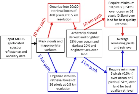
The only differences between the 3 km algorithm and the 10 km algorithm are the way the pixels are organized and the number of pixels required to proceed with a retrieval after all masking and deselection are accomplished. Figure 2 presents a flow chart showing the separate paths for the 10 km and 3 km retrievals. The black boxes running along the center of chart identify processes that are identical in both retrievals. The inputs are identical, as are the masking procedures. The exact same 0.5 km pixels identified as cloud, sediment, etc. in the 10 km algorithm are identified as cloud, sediment, etc. in the 3 km algorithm. The difference is in how the two al-gorithms make use of these 0.5 km designations. Once the 3 km algorithm has identified the pixels suitable for retrieval and decided that a sufficient number of these pixels remain, the spectral reflectances are averaged and the inversion con-tinues exactly the same as in the 10 km algorithm. The same assumptions are used, the same lookup tables, the same nu-merical inversion and the same criteria to determine a good fit.
1832 L. A. Remer et al.: MODIS 3 km aerosol product: algorithm and global perspective
! 1!
! 2!
! 3!
Input&MODIS& geolocated&
spectral& reflectance&and&
ancillary&data&
Organize&into&20x20& retrieval&boxes&of&& 400&pixels&at&0.5&km&&
resoluCon&
Organize&into&6x6& retrieval&boxes&of&& 36&pixels&at&0.5&km&&
resoluCon& Mask&clouds&and&
inappropriate& surfaces&
Arbitrarily&discard& darkest&and&brightest&
25%&over&ocean&and& darkest&20%&and& brightest&50%&over&
land&
Average& remaining&pixels&
and&retrieve& 10&km
&path &
3&km &path
&
Require&minimum& 10&pixels&(0.5km)& over&ocean&or&51& pixels&(0.5km)&over& land&for&best&quality&&
retrieval&
Require&minimum& 5&pixels&(0.5km)& over&ocean&or&5& pixels&(0.5km)&over&
land&for&best& quality&retrieval& 3&km
&path & &
10&km&path &
&
Fig. 2. Flowchart illustrating the different paths of the 10 km (red)
and 3 km (blue) retrievals. The procedures appearing in the black outlined boxes are common to both algorithms.
of 36), than what is required by the 10 km retrieval (2.5 %) for the best quality retrieval. The requirement over land is about the same in the 3 km retrieval as it is in the 10 km re-trieval (14% and 13%, respectively). For coastal rere-trievals, if any pixel in the 3 km retrieval box is “land” or “coastal”, then no ocean retrieval will be made. Furthermore, if there are 5 “land” pixels in the retrieval box, even if the remainder of the pixels are ocean, a land retrieval will be made, although qual-ity may be degraded depending on how many “water” pixels exist in the box.
Tables 1 through 3 list the parameters available in the MOD04 3K and MYD04 3K files. Readers are referred to Levy et al. (2013) and references therein for clarification of any parameter in these tables. Not all of the diagnostics available at 10 km are included at 3 km, but most of the pa-rameters are there. The data set includes an integer Quality Flag (Land Ocean Quality Flag) that designates each 3 km retrieval as “3”, “2”, “1” or “0”. The same recommenda-tions apply to the 3 km product as to the original product. Ocean retrievals are valid for all nonzero Quality Flags while land retrieval products are only recommended for Qual-ity Flags = “3”. The 3 km product also includes more de-tailed diagnostics about the retrieval embedded in the Qual-ity Assurance Ocean and QualQual-ity Assurance Land parame-ters. Note that the criteria to fill these quality diagnostics dif-fer slightly from the criteria used to fill the same-named pa-rameters at 10 km. Detailed information on the quality diag-nostics will be available in the Collection 6 Algorithm Theo-retical Basis Document available at http://modis-atmos.gsfc. nasa.gov/reference atbd.html.
The 3 km product is designed to provide insight into the aerosol situation on a focused local basis and will not be aggregated to the Level 3 global 1-degree grid. All Level 3 MODIS aerosol products will be derived from the 10 km product.
Table 1. Land and ocean parameters of the MOD/MYD04 3K file
and the parameter’s dimension.
Parameter dimension
Longitude (X, Y )
Latitude (X, Y )
Scan Start Time (X, Y )
Solar Zenith (X, Y )
Solar Azimuth (X, Y )
Sensor Zenith (X, Y )
Sensor Azimuth (X, Y )
Scattering Angle (X, Y )
Glint Angle (X, Y )
Land Ocean Quality Flag (X, Y )
Land sea Flag (X, Y ),
Optical Depth Land And Ocean (X, Y ) Image Optical Depth Land And Ocean (X, Y )
(X, Y )refers to a 2-dimensional array along and across the swath.
The 3 km retrieval should closely mirror the results of the 10 km retrieval because the majority of the two algo-rithms are identical, but it should be able to resolve gradi-ents across the 10 km retrieval box that would otherwise be missed. There is a possibility that the new algorithm will introduce additional noise, especially over land where pix-els representing inhomogeneous surfaces would have been eliminated in the deselection process of the larger box, but are now included in the retrieval. However, this tendency to-wards noise may be mitigated by the slightly more stringent requirements in deselection and the minimum number of pix-els needed to represent the box. The advantageous mitigation features will be more apparent over ocean than over land. Overall, the two algorithms provide different sampling of the aerosols over the globe and ,because of this alone, are not expected to provide the same global statistics.
3 Examples of results from 3 km algorithm
The 3 km algorithm was applied to six months of MODIS data from Aqua-MODIS: January and July 2003, 2008 and 2010. This is a special database of MODIS data used to test new MODIS algorithms before implementation into oper-ational production. The majority of the figures and analy-sis presented in this paper represents Test884, which is ex-pected to be nearly the final version before operational pro-cessing begins for MODIS atmospheres Collection 6 (Levy et al., 2013). Thus, the algorithm and product results shown in Figs. 3–14, and in Table 4, are our best estimate for the results of the soon-to-be-public Collection 6 MODIS aerosol products. However, there may still be small adjustments that deviate from Test884 when production actually begins.
(a) 10 km, 13:00 UTC
6 8 10 12 14 16
32 34 36
38 (b) 3 km, 13:00 UTC
6 8 10 12 14 16
32 34 36 38
AOD at 550 nm
-0.05 0.05 0.15 0.25 0.35 0.45 0.55 0.65 0.75
Fig. 3. Aerosol optical depth at 550 nm retrieved from the
15 July 2010 Aqua-MODIS radiances using the Collection 6 MODIS Dark Target aerosol algorithm. Left: the product at 10 km resolution. Right: the product at 3 km resolution. The situation is a moderate dust event over the Mediterranean Sea off the costs of Tunisia and Libya. The 3 km retrieval produces values closer to the coastline and to the islands.
the new 3 km product and how it differs from the 10 km prod-uct applied to exactly the same input data.
Figure 3 compares the 10 km and 3 km ocean retrievals over the Mediterranean Sea off the coast of Tunisia and Libya during a moderate dust event. The two resolution products produce almost the exact same aerosol field with the same gradient and same magnitude aerosol optical depth. This is because the two algorithms are essentially the same. The only difference is that the finer resolution product is able to make retrievals closer to the small islands in the image. We find that this is typical of the 3 km product. It offers over-ocean retrievals closer to land, nearer to islands and within narrow waterways and estuaries.
Figure 4 illustrates the apparent advantage of the 3 km product to resolve smoke plumes from fires. The fire is a large wild fire burning in Canada. The 10 km product does not capture the long narrow smoke plume leading towards the northwest, but the 3 km product does. One of the major advantages of the 3 km product is its ability to better resolve smoke plumes than the 10 km product. Even so, because the cloud identification algorithm in the 3 km product is the same as in the 10 km product, based primarily on spatial variability, the 3 km product still improperly confuses the thickest parts of the smoke plume with a cloud and mistakenly refuses to retrieve there.
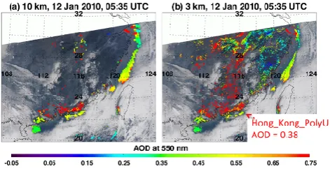
Figure 5 demonstrates the potential for different sam-pling by the two products. The situation is a highly pol-luted episode over much of southeastern China. Here the 3 km algorithm makes retrievals over a broad area, while the 10 km algorithm finds few opportunities to retrieve. The few places of overlap result in similar values of aerosol op-tical depth. The only AERONET station in the image is at Hong Kong PolyU (22◦180N, 114◦110E), which reports a collocated AOD interpolated to 0.55 µm at MODIS over-pass time of 0.38. The 10 km algorithm does not produce
Fig. 4. Same as Fig. 3 but for a situation over Canada where the
3 km product better resolves the plume from active wildfires. Note the additional red pixels between the clouds in the upper left corner of the image for the 3 km panel.
Fig. 5. Same as Fig. 3, but for 12 January 2010 during a pollution
episode in China. Here the 3 km algorithm is able to make retrievals over a much broader region. The AOD interpolated to 0.55 µm from the only AERONET station in the image (Hong Kong PolyU) is 0.38. The 3 km retrieval there is 0.45, while there is no 10 km re-trieval available at that spot during this overpass.
a retrieval at this station, but the 3 km algorithm does, pro-ducing an AOD of 0.45, a reasonable match. The colloca-tion procedure and quantificacolloca-tion of expected uncertainties are described in Sect. 5 below.
1834 L. A. Remer et al.: MODIS 3 km aerosol product: algorithm and global perspective
Table 2. Ocean parameters of the MOD/MYD04 3K file and the parameter’s dimension.
Parameter dimension
Wind speed Ncep Ocean (X, Y )
Solution Index Ocean Small (X, Y )
Solution Index Ocean Large (X, Y )
Effective Optical Depth Best Ocean (X, Y,7); 0.47, 0.55, 0.66, 0.86, 1.24, 1.63, 2.11 µm Effective Optical Depth Average Ocean (X, Y,7); 0.47, 0.55, 0.66, 0.86, 1.24, 1.63, 2.11 µm Optical Depth Small Best Ocean (X, Y,7); 0.47, 0.55, 0.66, 0.86, 1.24, 1.63, 2.11 µm Optical Depth Small Average Ocean (X, Y,7); 0.47, 0.55, 0.66, 0.86, 1.24, 1.63, 2.11 µm Optical Depth Large Best Ocean (X, Y,7); 0.47, 0.55, 0.66, 0.86, 1.24, 1.63, 2.11 µm Optical Depth Large Average Ocean (X, Y,7); 0.47, 0.55, 0.66, 0.86, 1.24, 1.63, 2.11 µm
Mass Concentration Ocean (X, Y )
Aerosol Cloud Fraction Ocean (X, Y )
Effective Radius Ocean (X, Y,2): best, average
PSML003 (X, Y,2): best, average
Asymmetry Factor Best Ocean (X, Y,7); 0.47, 0.55, 0.66, 0.86, 1.24, 1.63, 2.11 µm Asymmetry Factor Average Ocean (X, Y,7); 0.47, 0.55, 0.66, 0.86, 1.24, 1.63, 2.11 µm Backscattering Ratio Best Ocean (X, Y,7); 0.47, 0.55, 0.66, 0.86, 1.24, 1.63, 2.11 µm Backscattering Ratio Average Ocean (X, Y,7); 0.47, 0.55, 0.66, 0.86, 1.24, 1.63, 2.11 µm Angstrom Exponent 1 Ocean (0.55/0.86 micron) (X, Y,2): best, average
Angstrom Exponent 2 Ocean (0.86/2.1 micron) (X, Y,2): best, average Least Squares Error Ocean (X, Y,2): best, average Optical Depth Ratio Small Ocean 055micron (X, Y,2): best, average
Optical Depth by models (X, Y,9): 9 models
Number Pixels Used Ocean (X, Y )
Mean Reflectance Ocean (X, Y,7); 0.47, 0.55, 0.66, 0.86, 1.24, 1.63, 2.11 µm STD Reflectance Ocean (X, Y,7); 0.47, 0.55, 0.66, 0.86, 1.24, 1.63, 2.11 µm
Quality Assurance Ocean (X, Y ); Packed byte
X, Yrefers to a 2-dimensional array along and across the swath. Some parameters have a third dimension. A dimension of “7” refers to the 7 retrieved ocean wavelengths, listed. A dimension of “2” refers to either the solution with minimum fitting error (best) or the average of all solutions with fitting error less than 3 % (average) (Remer et al., 2005). A dimension of “9” refers to the 9 models, 4 fine mode and 5 coarse mode, used in the retrieval (Remer et al., 2005).
this occurs most frequently over urban surfaces, a type of lo-cation of most interest to the air quality community.
4 Global mean aerosol statistics of the 3 km product
The global mean aerosol optical depth calculated from the 10 km and 3 km algorithms are different because the two al-gorithms sample differently. In general the global statistics of the 3 km product tracks the day-to-day variation of the 10 km product. Figure 7 shows the day-to-day global mean AOD differences between the two products over ocean and land for the three months of January merged into one continuous time series for plotting purposes and the three July months merged into one another. In this figure global means are cal-culated from a straight averaging of all retrievals on any day. There is no pixel or area weighting, and no gridding to a map to preserve spatial structure. A positive difference indi-cates that the 3 km AOD is higher than the 10 km AOD. The differences in global monthly mean AOD between the two resolution data sets is−0.004 in January and nearly 0.000 in July over ocean and 0.004 in January and 0.010 in July over land. The largest day to day differences between the products
Fig. 6. Same as in Fig. 3 but for a situation over California where
the 3 km product introduces widespread artificial noise over an ur-ban area that the 10 km product better confines. There were no col-locations with AERONET for this image.
Table 3. Land parameters of the MOD/MYD04 3K file and the parameter’s dimension.
Parameter dimension
Aerosol Type Land (X, Y )
Fitting Error Land (X, Y )
Surface Reflectance Land (X, Y,3); 0.47, 0.66, 2.11 µm Corrected Optical Depth Land (X, Y,3∗); 0.47, 0.55, 0.66 µm Corrected Optical Depth Landwav2p1 (X, Y )
Optical Depth Ratio Small Land (X, Y )
Number Pixels Used Land (X, Y )
Mean Reflectance Land (X, Y,7); 0.46, 0.55, 0.66, 0.86, 1.24, 1.63, 2.11 µm STD Reflectance Land (X, Y,7); 0.46, 0.55, 0.66, 0.86, 1.24, 1.63, 2.11 µm
Mass Concentration Land (X, Y )
Aerosol Cloud Fraction Land (X, Y )
Quality Assurance Land (X, Y )
Topographic Altitude Land (X, Y )
X, Yrefers to a 2-dimensional array along and across the swath. Some parameters have a third dimension. A dimension of “3” refers to the 3 wavelengths of input reflectances used in the retrieval, listed. A dimension of “3∗” refers to the 3 retrieved wavelengths over land, listed. A dimension of “7” refers to the 7 solar wavelengths, listed.
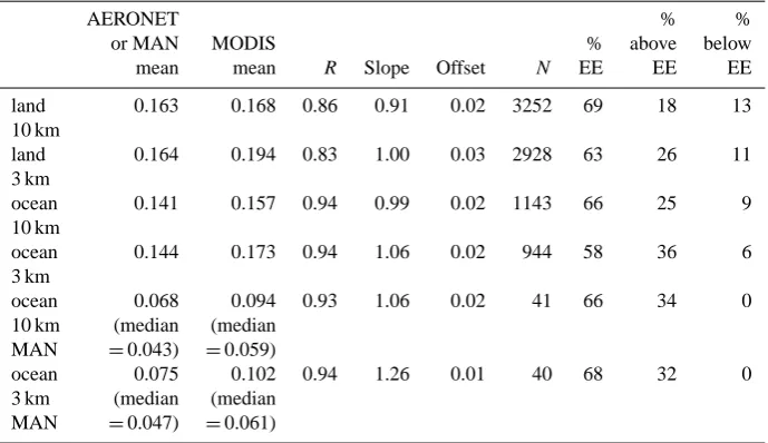
Table 4. Parameters from MODIS-AERONET collocation validation: means of each data set, correlation coefficient, regression slope and
offset, number of collocations, percent within expected error∗, percent above expected error∗and percent below expected error∗for 10 km and 3 km products separated into land and ocean retrievals. The last rows show MODIS-MAN collocations over ocean.
AERONET % %
or MAN MODIS % above below
mean mean R Slope Offset N EE EE EE
land 0.163 0.168 0.86 0.91 0.02 3252 69 18 13
10 km
land 0.164 0.194 0.83 1.00 0.03 2928 63 26 11
3 km
ocean 0.141 0.157 0.94 0.99 0.02 1143 66 25 9
10 km
ocean 0.144 0.173 0.94 1.06 0.02 944 58 36 6
3 km
ocean 0.068 0.094 0.93 1.06 0.02 41 66 34 0
10 km (median (median MAN =0.043) =0.059)
ocean 0.075 0.102 0.94 1.26 0.01 40 68 32 0
3 km (median (median
MAN =0.047) =0.061)
∗Expected error for land is±0.05±0.15AOD, and for ocean it is±0.03±0.05AOD.
as compared with July. The large daily difference in the prod-ucts in January over land, corresponding to Day 12 on 2010 on the graph (12 January 2010), does not correspond to an unusual spike in global land AOD, just to a large difference between the two products. On this day the differences are concentrated in a handful of granules, of which the most dra-matic is the 05:35 UTC granule shown in Fig. 5. Likewise, other spikes on the difference plots are not associated with unusual global mean AOD.
Figure 8 shows the scatter plots of the 3 km daily global mean over land and ocean plotted against the same using the 10 km product. These are the same data from Fig. 7. The
1836 L. A. Remer et al.: MODIS 3 km aerosol product: algorithm and global perspective
! 1!
Fig. 7. Difference between 3 km daily global mean aerosol
opti-cal depth (AOD) at 550 nm and the same at 10 km for over ocean (left) and over land (right). Positive differences indicate that the 3 km AOD is higher than the 10 km AOD.
the 3 km product actually tends towards higher AOD. As of now we do not have an explanation for these tendencies in the global mean AOD statistics over ocean.
Figure 9 shows the histograms calculated from the six months of data described in Sect. 3, with all months of Jan-uary combined and all months of July combined, land and ocean separately. These histograms are constructed from in-dividual retrieval boxes accumulated for the entire three-month periods with no spatial or diurnal averaging. The his-tograms are plotted with relative frequency rather than total number of retrievals in each bin because the 3 km product at finer spatial resolution produces approximately 11 times and 7 times the number of retrievals produced by the 10 km prod-uct, over land and ocean, respectively. Here we see over land with the 3 km product a decrease in the proportion of nega-tive and very low AOD retrievals and an increase in retrievals in the 0.10–0.30 range in January and in the AOD above 0.15 in July. This shift is more apparent in Fig. 10. The overall in-crease in global mean AOD over land with the 3 km product noted in Figs. 7 and 8 appears to be due to shifting to moder-ate and higher AOD from very low AOD and not only from introducing spikes at very high AOD. In contrast, over ocean the histograms show an increase in very low AOD (0–0.05) at the expense of slightly higher AOD (0.05–0.15 or 0.20). Fig-ure 10 clarifies the differences between the 3 km and 10 km histograms.
There are two reasons why 3 km and 10 km daily global mean AOD or histograms may differ in Figs. 7–10. First, the different algorithms may be retrieving different values of AOD when both retrieve in the same location. Second, the global sampling may be very different with the 3 km product retrieving in locations that the 10 km product does not, as in Fig. 5. We explore these two possibilities by examining the differences in the global distribution of monthly mean AOD in both resolutions.
Figure 11 shows the global distribution of the July 2008 monthly mean AOD for the 3 km and 10 km retrievals. These plots are created by first gridding the granule-level retrievals onto a daily 1◦×1◦latitude/longitude global grid. Each grid
!
Fig. 8. Daily global mean aerosol optical depth (AOD) at 550 nm for
the 93 days of the months of January, and 93 days of the months of July 2003, 2008 and 2010 calculated from the 3 km product plotted against the same calculations used in the 10 km product. The left plot is for ocean, and the right plot is for land. Note the different scales on the axes for the ocean and land plots.
cell contains the mean of all high quality AOD retrievals in that grid cell on that day. There is no minimum number of retrievals required in the 1-degree box in order to fill that box each day. Then, the monthly mean map is calculated by adding the AOD in each box from each daily map and divid-ing by the number of days. The monthly mean is a straight average of the days and is not pixel-weighted; however, the number of pixels in each grid box is retained. There must be a total of 10 retrievals over the entire month for that grid cell to be considered “filled”. Because no minimum threshold is set in filling the grid boxes on the daily maps, a grid box can be filled even if one lone pixel is retrieved, and this one lone pixel can propagate up to the monthly mean. This process of creating the monthly means will accentuate the contribution of outliers (Levy et al., 2009), and will accentuate the dif-ferences between fine and coarse resolution products, in our case the 3 km and 10 km products.
The July 2008 monthly mean 3 km AOD is clearly higher than the 10 km AOD over land areas in Fig. 11, especially in the Northern Hemisphere and across the tropical belt. Mostly these areas exhibit AOD∼0.05 to 0.10 in the 10 km plot, but turn to ∼0.15 to 0.25 in the 3 km, in agreement with the difference histogram of Fig. 10. The differences in the two maps are highlighted in the difference map of Fig. 11c. However, some of the AOD increase from 10 km to 3 km is due to the increase in the number of grid squares reporting AOD in high AOD regions, such as India, moderately high AOD regions such as China and southeast Asia. This increase in reporting additional grid squares corresponds to some of the increase at high AOD in Fig. 10.
!
Fig. 9. Frequency histograms of 10 km and 3 km AOD retrievals,
constructed from global retrievals from three months of January (2003, 2008 and 2010) in the left column and from three months of July (same years) in the right column. Land in the top row and ocean in the bottom. Bin labels represent the lower boundary of the bin. Note a scale break in the x axis. Bin widths below 0.3 are 0.05. Above 0.3, widths increase and are variable: 0.3 to 0.4, 0.4 to 0.5, 0.5 to 0.7, 0.7 to 1.0, 1.0 to 1.5, 1.5 to 2 and 2 to 3.
sufficient to create the relative increase of very low AOD in the histograms. The other months were analyzed with simi-lar results. In January the patterns seen in the July monthly mean maps swap hemispheres, but are otherwise similar.
Thus, overall the 3 km product tracks the 10 km product on a day-to-day basis, although the product over land tends to be higher than the 10 km product, and over the ocean lower. There is seasonal variation to these tendencies. The 3 km in-crease in AOD over land is caused by both higher AOD in the same 1-degree grid squares where both algorithms pro-duce a monthly mean, but also by an increase in the number of reporting grid squares in high to moderate AOD regions. Over ocean, the decrease is also a combination of lower AOD retrievals in high AOD regions and the addition of new filled grid squares with very low values.
5 Global validation
The six months of test data described above (January and July 2003, 2008 and 2010) were collocated with Level 2.0 AERONET observations to test the accuracy of the retrievals. For the 10 km retrievals, we use the Petrenko et al. (2012) protocol for collocations, which differs slightly from the one introduced in Ichoku et al. (2002). Here, a collocation is the
-0.02 -0.01 0 0.01 0.02 0.03 0.04
0 0.2 0.4 0.7 1
Jan land
July land Jan ocean
July ocean
fre
q
di
ffe
re
nce
(
3km
-
10
km)
AOD bin
0.1 0.3 0.5
!
Fig. 10. Bin by bin differences between the frequency histograms
of Fig. 9 (3–10 km).
1838 L. A. Remer et al.: MODIS 3 km aerosol product: algorithm and global perspective
Fig. 11. Spatially distributed monthly mean AOD for July 2008 for
10 km, upper left; 3 km upper right; the difference (3–10 km) and the AOD of grid squares added to the 10 km map by the 3 km re-trieval.
in order to match MODIS. A quadratic fit in log-log space is used to make the interpolation (Eck et al., 1999).
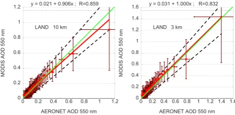
Figure 12 shows the binned scatter plots from six months of collocations for land. There are 3252 collocations at 10 km and 2928 at 3 km. The data were sorted accord-ing to AERONET AOD and bins designated for every 50 collocations. The mean and standard deviation of both the AERONET and MODIS AODs were calculated. The mean values for each bin are plotted and the error bars indicate ±1 standard deviation. The red line represents the linear regres-sion calculated for the full data set of approximately 3000 collocations and not the roughly 60 bins plotted in the figure. The dashed lines indicate the “expected error” (Levy et al., 2010). For land the expected error is
1AOD= ±0.05±0.15 AOD. (1)
Table 4 provides the mean AOD of each data set, the corre-lation coefficient, the regression statistics and the number of MODIS retrievals that fall within expected error, fall above the expected error bound (the upper dashed line) and fall below the expected error bound (the lower dashed line in Fig. 12).
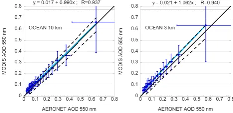
Figure 13 shows similar binned scatter plots for the ocean retrieval. There are fewer ocean collocations, 1143 at 10 km and 944 at 3 km. Because AERONET stations are generally on land, the 10 km retrieval with its longer radius will inter-cept more ocean retrievals than the 3 km retrieval with only a 7.5 km radius. The expected error for ocean is
0 0.2 0.4 0.6 0.8 1 1.2
0 0.2 0.4 0.6 0.8 1 1.2
MO
D
IS
AO
D
5
50
n
m
AERONET AOD 550 nm LAND 10 km y = 0.021 + 0.906x ; R=0.859
0 0.2 0.4 0.6 0.8 1 1.2 1.4 1.6
0 0.2 0.4 0.6 0.8 1 1.2 1.4 1.6
MO
D
IS
AO
D
5
50
n
m
AERONET AOD 550 nm LAND 3 km
y = 0.031 + 1.000x ; R=0.832
!
Fig. 12. Binned scatter plot of MODIS AOD at 550 nm retrieved
from over land against AERONET observed AOD. MODIS 10 km product on the left and 3 km product on the right. Each bin repre-sents 50 collocations. AERONET AOD has been interpolated to this wavelength to match MODIS. Error bars represent±1 standard de-viation in the bin. The green line is the 1 : 1 line. The red line is the linear regression through the full database of 3252 and 2928 collo-cations for 10 km and 3 km, respectively. The dashed lines represent expected error of the MODIS 10 km retrieval. The range of the axes in each plot are different. Regression statistics are given in Table 4.
1AOD= ±0.03±0.05 AOD. (2)
These figures show that the 10 km product of this six-month database is meeting its expectations with most retrievals falling within expected error (69 % over land and 66 % over ocean). Correlations are high (0.86 over land and 0.94 over ocean) and most retrievals and the linear regression fall close to the 1 : 1 line. The land retrieval does show a positive bias of∼0.005 and the ocean∼0.016, but these are well-within expected uncertainties.
The 3 km product is also highly correlated to AERONET observations and most of the 3 km retrievals fall within the expected error bounds. However, the 3 km product matches AERONET less well than does the 10 km MODIS product. The most obvious degradation of accuracy between the 3 km and 10 km products is over ocean where the finer resolu-tion product has developed a positive bias of almost 0.03 with only 58 % of retrievals falling within the expected error bounds. The land retrieval has also significantly increased its positive bias against AERONET at finer resolution. In addi-tion to the increased bias, the 3 km land product introduces additional noise at low AOD. This can be seen in the degra-dation of the correlation coefficient in Table 4.
0 0.1 0.2 0.3 0.4 0.5 0.6 0.7 0.8
0 0.1 0.2 0.3 0.4 0.5 0.6 0.7 0.8
MO
D
IS
AO
D
5
50
n
m
AERONET AOD 550 nm OCEAN 10 km
y = 0.017 + 0.990x ; R=0.937
0 0.1 0.2 0.3 0.4 0.5 0.6 0.7 0.8
0 0.1 0.2 0.3 0.4 0.5 0.6 0.7 0.8
MO
D
IS
AO
D
5
50
n
m
AERONET AOD 550 nm OCEAN 3 km
y = 0.021 + 1.062x ; R=0.940
!
Fig. 13. Same as Fig. 12, but for over ocean retrieval. Here, the
linear regression line is in light blue and the 1 : 1 line is in black.
retrievals during the six months of this test data set, in Jan-uary and July, 2003, 2008 and 2010. A collocation was de-fined using the same spatial averaging and minimum number of MODIS retrieval criteria as with a MODIS-AERONET collocation. The MAN measurements temporally average a series of measurements together to form one measurement. All “series” measurements within a half hour of the MODIS overpass are temporally averaged. Due to the limited amount of MAN data, there was no minimum number of MAN “se-ries” measurements required to create a collocation. Only ocean retrievals with a QA ≥1 are included in the collo-cation. Because of the requirement that there be at least 2 or 20 % of available retrievals within a 7.5 km radius for the 3 km product and a 25 km radius for the 10 km product, the two sets of collocations do not necessarily contain the same points. In our sets of MAN-MODIS collocations there are 40 collocations at 3 km and 41 collocations at 10 km, of which 30 are common to both resolutions and 10 and 11 are unique for each resolution, respectively. The AERONET collocation exercise also results in differently sampled data sets, but the results of this different sampling is much more apparent in the MAN process because of the small statistical sampling size.
The results of the MODIS-MAN collocations are shown in Fig. 14. Most MAN collocations occurred in very clean en-vironments with the exception of 3 points (only 2 at 10 km) that occurred in the tropical Atlantic in the dust belt and a moderate value near AOD∼0.2 from the Hudson Bay that appears to be wildfire smoke. The highest AOD collocation in the 3 km database (9 July 2008 from the dust belt of the Atlantic Ocean with MODIS AOD = 0.67) does not appear in the 10 km database. Most of the MODIS 3 km points agree with the MAN observations to within expectations. The ex-ceptions include that one high dust point and a group of col-locations at low AOD that are all traced to a specific cruise within sight of the Antarctic coast in January 2008. The re-gression and correlation statistics are given in Fig. 14 and in Table 4 but because of the outlying dust point in the 3 km set, these statistics are not robust descriptions of the bulk of the observations. For example while the mean AODs of the
Fig. 14. Scatter plot of MODIS 10 km and 3 km retrievals of AOD at
550 nm plotted against collocated data from the Maritime Aerosol Network (MAN). At 10 km and 3 km, 41 and 40 collocations were identified, respectively, in the 6 months undergoing analysis.
MAN and MODIS populations are 0.075 and 0.102, respec-tively, the medians are 0.047 and 0.061, respectively. The 40 and 41 points are inadequate to fully represent the relation-ship between MODIS 3 km retrievals over the wide variety of conditions experienced over the world’s oceans. They are shown here to supplement the other inadequate data set of the AERONET coastal and island sites. Together the avail-able ocean validation does suggest, without firm proof, that the ocean 3 km retrieval will approach similar levels of uncer-tainty as the well-studied ocean 10 km product, but introduce some additional noise.
The choices of temporal and spatial averaging windows in the spatio-temporal collocation analysis are somewhat ar-bitrary and based on previous work with the 10 km product (Ichoku et al., 2002; Petrenko et al., 2012). We chose to re-duce the spatial averaging window of the 3 km product in or-der to test this finer resolution product at scales more appro-priate to its expected applications. In order to test our deci-sion, we calculated collocation statistics for the 3 km product using a previous version of the retrieval algorithm (Test811) applied to the same set of 6 months used in the above anal-ysis, and vary both the spatial and temporal windows as a sensitivity test. There are many differences in the basic re-trieval between Test811 and the version used in all the above analysis (Test884) including different gas correction, cloud screening, surface reflectance parameterization, etc. All of these affect the retrieved AOD, but are not specific to the 3 km retrieval specifically. The results of the Test881 sen-sitivity test, shown in Table 5, are internally consistent but cannot be compared with those in Table 4 or in any of the figures.
1840 L. A. Remer et al.: MODIS 3 km aerosol product: algorithm and global perspective
Table 5. Same as Table 4, but using results from a different version of the MODIS aerosol algorithm (Test881) and for a variety of temporal
and spatial averaging windows in the collocation between the 3 km retrieval and AERONET.
Land % %
or 1x 1t AERONET MODIS % above below
ocean (km) (min) Mean Mean R Slope Offset N EE EE EE
land 7.5 15 0.131 0.168 0.83 0.997 0.04 794 62 29 9
land 7.5 30 0.144 0.189 0.84 1.069 0.03 2674 62 31 7
land 7.5 60 0.152 0.201 0.84 1.046 0.04 3280 62 31 7
land 25 15 0.129 0.149 0.88 0.944 0.03 1081 71 21 8
land 25 30 0.139 0.164 0.86 0.971 0.03 3611 71 22 7
land 25 60 0.149 0.175 0.86 0.961 0.03 4513 70 23 7
ocean 7.5 15 0.135 0.145 0.91 0.91 0.02 145 66 24 10
ocean 7.5 30 0.134 0.147 0.93 0.936 0.02 495 70 23 7
ocean 7.5 60 0.136 0.149 0.93 0.959 0.02 626 70 23 7
ocean 25 15 0.129 0.145 0.90 1.048 0.01 449 67 24 9
ocean 25 30 0.147 0.170 0.93 1.127 0.0 1507 66 26 8
ocean 25 60 0.152 0.171 0.93 1.086 0.0 1915 67 25 8
∗Expected error for land is±0.05±0.15AOD, and for ocean it is±0.03±0.05AOD.
over ocean. We find that broader spatial averaging mitigates some of the noise introduced in the 3 km product over land, but over the ocean there is less noise and that distance from the land-based AERONET station causes degradation in the correlation. However, mostly the spatial and temporal aver-aging windows matter little to the validation conclusions.
6 Discussion and conclusions
The MODIS Dark Target aerosol algorithm relies on a data selection process that identifies a relatively few ideal pix-els to use in the retrieval of aerosol optical depth and other aerosol characteristics. By choosing only a few pixels to rep-resent aerosol over a moderate resolution retrieval box, noise is reduced and situations difficult to retrieve are avoided. Inherent in this selection procedure is an assumption that aerosol properties do not vary across the retrieval box, so that the aerosol conditions across the box can be represented by just a small fraction of pixels. Except for specific situations near sources: smoke plumes from fires, dust plumes from playas, etc., aerosol homogeneity over mesoscale lengths of 40–400 km has been considered to be a robust assumption (Anderson et al., 2003). The 10 km (nadir) to 40 km (swath edge) retrieval is a reasonable algorithm construct, given this understanding of aerosol homogeneity. However, as our op-portunities to observe aerosols increase and our understand-ing grows, we know now that aerosols may vary frequently over much smaller spatial scales (Shinozuka and Redemann, 2011; Munchak et al., 2013, this issue). Not only will the 10 km retrieval box lose the details of local variability, the assumption on which it is based may be in error.
Because there is need for finer resolution aerosol prod-ucts to resolve individual plumes and fine gradients, the MODIS Science Team is introducing a 3 km product in their
Collection 6 delivery. This product will be available at the granule level, in separate files labeled as MOD04 3K and MYD04 3K, for Terra and Aqua, respectively. The new prod-uct differs from the original 10 km prodprod-uct only in the man-ner in which reflectance pixels are ingested, organized and selected by the aerosol algorithm. All cloud, surface, sedi-ment, snow and ice masking remain identical to the original algorithm, and lookup tables and inversion methods have not changed. The only difference is in how the algorithm arbi-trarily discards additional good pixels to obtain the best pix-els for retrieval. In the 3 km algorithm, pixpix-els will be used for retrieval that would have been arbitrarily discarded by the 10 km algorithm.
The 3 km product exhibits expected characteristics. It re-solves aerosol plumes and details of fine-scale gradients that the 10 km product misses. In some situations it provides re-trievals over entire regions that the 10 km barely samples. The 3 km product also allows the ocean retrieval to retrieve closer to islands and in narrow bays. On the other hand, in situations known to be difficult for the Dark Target retrieval, such as over bright surfaces and especially over urban sur-faces, the 3 km retrieval introduces sporadic unrealistic high values of AOD that are avoided more successfully by the 10 km retrieval. We can label these artifacts as “noise”, but it is not random noise because the tendency over land is to over estimate AOD in these artifacts.
resolution product. This would suggest that the 3 km global mean AOD is a truer representation of the global mean. On the other hand, the 3 km product introduces a high-biased noise over bright and/or urban surfaces, and so, the global mean from the 10 km product would remain the truer rep-resentation. Collocations with AERONET observations sug-gest the latter. The 3 km AOD over land compares less well with AERONET than does the 10 km AOD, decreasing cor-relation, increasing high bias and shifting retrievals from within expectations of uncertainty to exceeding those expec-tations. We conclude that the 3 km AOD over land is less ac-curate and less robust than the 10 km AOD. Estimated uncer-tainty of the 3 km land product, based on 6 months of colloca-tions with AERONET, suggest that 66 % of retrievals should fall within
1AOD 3 km= ±0.05±0.20 AOD (3) with the understanding that most retrievals will fall within the positive end of this error bounding, leaving a positive bias.
Over the ocean, globally, the 3 km algorithm picks up pro-portionally a greater number of very low AOD cases than the 10 km algorithm. Again, just from comparing the two MODIS resolution products we cannot tell whether this low bias is a better representation of global AOD or not. Un-fortunately, the comparison with AERONET cannot either. AERONET stations used for the over ocean validation are isolated to a limited number of island and coastal locations. The very low AOD situations tend to occur over open ocean. The AERONET analysis suggests that the 3 km algorithm in-troduces positive bias, not negative. This is because the 3 km product retrieves closer to shore, where the AERONET sta-tion is located. In these locasta-tions, likelihood of sediment con-tamination is high, aerosol is continental in nature and we expect that the result of the AERONET validation over the ocean is not applicable to the global oceanic AOD retrieval. Nor can we come to a conclusion about the relative accuracy of the two products in the coastal zone, because the validation procedure enables the 10 km product to encompass retrievals much further from the shore than the 3 km product. However, in the coastal zone, within 7.5 km of shore, we conclude that 69 % of 3 km retrievals should fall within
1AOD 3 km= ±0.04±0.05 AOD; (4) moreover, with an understanding similar to the land error bars that most retrievals will fall in the positive end of this error bounding leading to positive biases.
The data from the MAN cruises were also inadequate to state firm conclusions about the 3 km ocean retrieval because only 40 collocations were identified in the analysis data set, and several of those points were highly localized to spe-cific locations such as Hudson Bay and near the Antarctic coast. However, even in this limited data set, 68 % of the 3 km retrievals were contained within the same error bounds stated for the 10 km ocean retrieval,1AOD 3 km =±0.03±
0.05 AOD.
All analysis presented in this paper represent Aqua-MODIS from a limited 6 month analysis data set. Subse-quently, Terra-MODIS data from the same 6 months were also examined, and no results from the Terra analysis contra-dict the conclusions presented here.
We have made no attempt in this analysis to address cloud effects on the 3 km retrieval. Some of the high bias seen in the over land product could be due to additional cloud contami-nation and cloud effects in the product instead of artifacts in-troduced by bright surfaces. However, the fact that the ocean 3 km product also does not contain this high bias prompts us towards considering surface effects and not clouds, but with-out further analysis we cannot make firm conclusions. Future work will definitely need to address cloud 3-D effects (Wen et al., 2007; Marshak et al., 2008), the so-called twilight zone or continuum (Koren et al., 2007; Charlson et al., 2007), and other cloud issues on the finer resolution aerosol product.
Overall the 3 km product mimics the 10 km product, glob-ally, and on a granule-by-granule basis. Because the new product is essentially the same as the traditional Dark Target product, it is well understood and the limited analysis pre-sented above is sufficient to recommend its use by the com-munity with the following caveats:
– Global studies should continue to make use of the more
robust and well-studied 10 km product. The 3 km prod-uct’s use should be restricted to obvious situations that require finer resolution.
– Only the AOD at 550 nm was examined in this study.
Differences in the spectral AOD and size parameter re-trievals over ocean in the two resolution products are possible.
– Aerosol-cloud studies with the 3 km product should
pro-ceed cautiously. At this time, we do not specifically know how the 3 km product is affected in the proxim-ity of clouds.
– While the air quality community will be eager to apply
the 3 km product across an urban landscape, this must proceed cautiously because of known artifacts in the product over urban surfaces. See Fig. 6 and Munchak et al. (2013).
The power of the new product is on the local scale, not the global one, as was studied here. Future work that applies the MODIS 3 km aerosol product to local aerosol situations in case studies and evaluates the results will be necessary to continue the work started here (ie. Munchak et al., 2013). We expect the new 3 km product to provide important informa-tion complementary to existing satellite-derived products and become an important tool for the aerosol community.
1842 L. A. Remer et al.: MODIS 3 km aerosol product: algorithm and global perspective
federation who continue to provide a gold standard of aerosol characterization, unselfishly sharing their information with all. We also thank Dr. Jun Wang and the anonymous reviewer for their helpful comments, and again thanks to the pair of reviewers and to Dr. Michael King who served as editor of this paper for their extreme patience as we struggled to meet editorial deadlines.
Edited by: M. King
References
Ackerman, S., Frey, R. A., Strabala, K., Liu, Y., Gumley, L., Baum, B., and Menzel, P.: Discriminating clear sky from clouds with MODIS, Algorithm Theoretical Basis Document (MOD35), Version 6.1., available at: http://modis-atmos.gsfc. nasa.gov/reference atbd.html (last access: 29 July 2013), Octo-ber 2010.
Al-Saadi, J., Szykman, J., Pierce, R. B., Kittaka, C., Neil, D., Chu, D. A., Remer, L., Gumley, L., Prins, E., Weinstock, L., MacDon-ald, C., Wayland, R., Dimmick, F., and Fishman, J.: Improving national air quality forecasts with satellite aerosol observations, B. Am. Meteorol. Soc., 86, 1249–1264, doi:10.1175/BAMS-86-9-1249, 2005.
Anderson, T. L., Charlson, R. J., Winker, D. M., Ogren, J. A., and Holmen, K.: Mesoscale variations of tropospheric aerosols. J. Atmos. Sci., 60, 119–136, doi:10.1175/1520-0469(2003)060<0119:MVOTA>2.0.CO;2, 2003.
Charlson, R. J., Ackerman, A. S., Bender, F. A.-M., Anderson, T. L., and Liu, Z.: On the climate forcing consequences of the albedo continuum between cloudy and clear air, Tellus B., 59, 715–727, doi:10.1111/j.1600-0889.2007.00297.x, 2007.
Christopher, S. A., Zhang, J., Kaufman, Y. J., and Remer, L. A.: Satellite-based assessment of top of atmosphere anthropogenic aerosol radiative forcing over cloud-free oceans, Geophys. Res. Lett., 33, L15816, doi:10.1029/2005GL025535, 2006.
Chu, D. A., Kaufman, Y. J., Zibordi, G., Chern, J. D., Mao, J., Li, C., and Holben, B. N.: Global monitoring of air pollution over land from EOS-Terra MODIS, J. Geophys. Res., 108, 4661, doi:10.1029/2002JD003179, 2003.
De Almeida Castanho, A. D., Vanderlei, J. M., and Artaxo, P.: MODIS aerosol optical depth Retrievals with high spatial resolu-tion over an urban area using the critical reflectance, J. Geophys. Res.-Atmos., 113, D02201, doi:10.1029/2007JD008751, 2008. Eck, T. F., Holben, B. N., Reid, J. S., Dubovik, O., Smirnov, A.,
O’Neill, N. T., Slutsker, I., and Kinne, S.: Wavelength depen-dence of the optical depth of biomass burning, urban and desert dust aerosols, J. Geophys. Res., 104, 31333–31350, 1999. Engel-Cox, J. A., Holloman, C. H., Coutant, B. W., and Hoff, R. M:
Qualitative and quantitative evaluation of MODIS satellite sensor data for regional and urban scale air quality, Atmos. Environ., 38, 2495–2509, doi:10.1016/j.atmosenv.2004.01.039, 2004. Frey, R. A., Ackerman, S. A., Liu, Y., Strabala, K. I., Zhang, H.,
Key, J., and Wang, X.: Cloud Detection with MODIS, Part I: Recent Improvements in the MODIS Cloud Mask, J. Tech., 25, 1057–1072, 2008.
Gao, B.-C., Kaufman, Y. J., Tanre, D., and Li, R.-R.: Distinguishing tropospheric aerosol from thin cirrus clouds for improved aerosol retrievals using the ratio of 1.38 µm and 1.24 µm channels, Geo-phys. Res. Lett., 29, 1890, doi:10.1029/2002GL015475, 2002.
Hsu, N. C., Tsay, S. C., King, M. D., and Herman, J. R.: Aerosol properties over bright-reflecting source regions, IEEE T. Geosci. Remote, 42, 557–569, doi:10.1109/TGRS.2004.824067, 2004. Ichoku, C., Chu, D. A., Mattoo, S., Kaufman, Y. J., Remer,
L. A., Tanr´e, D., Slutsker, I., and Holben, B. N.: A spatio-temporal approach for global validation and analysis of MODIS aerosol products, Geophys. Res. Lett., 29, MOD1.1–MOD1.4, doi:10.1029/2001GL013206, 2002.
Kaufman, Y. J., Tanr´e, D., Remer, L. A., Vermote, E. F., Chu, A., and Holben, B. N.: Operational remote sensing of tropospheric aerosol over land from EOS moderate resolution imaging spec-troradiometer, J. Geophys. Res., 102, 17051–17067, 1997. Kaufman, Y. J., Tanre, D., and Boucher, O.: A satellite view of
aerosols in the climate system, Nature, 419, 215–223, 2002. Kaufman, Y. J., Boucher, O., Tanr´e, D., Chin, M., Remer, L.
A., and Takemura, T.: Aerosol anthropogenic component es-timated from satellite data, Geophys. Res. Lett., 32, L17804, doi:10.1029/2005GL023125, 2005a.
Kaufman, Y. J., Koren, I., Remer, L. A., Tanr´e, D., Ginoux, P., and Fan, S.: Dust transport and deposition observed from the Terra-MODIS spacecraft over the Atlantic Ocean, J. Geophys. Res., 110, D10S12, doi:10.1029/2003JD004436, 2005b.
Kaufman, Y. J., Koren, I., Remer, L. A., Rosenfeld, D., and Rudich, Y.: The Effect of Smoke, Dust and Pollution Aerosol on Shallow Cloud Development Over the Atlantic Ocean, P. Natl. Acad. Sci., 102, 11207–11212, 2005c.
Kinne, S., Schulz, M., Textor, C., Guibert, S., Balkanski, Y., Bauer, S. E., Berntsen, T., Berglen, T. F., Boucher, O., Chin, M., Collins, W., Dentener, F., Diehl, T., Easter, R., Feichter, J., Fillmore, D., Ghan, S., Ginoux, P., Gong, S., Grini, A., Hendricks, J., Herzog, M., Horowitz, L., Isaksen, I., Iversen, T., Kirkev˚ag, A., Kloster, S., Koch, D., Kristjansson, J. E., Krol, M., Lauer, A., Lamarque, J. F., Lesins, G., Liu, X., Lohmann, U., Montanaro, V., Myhre, G., Penner, J., Pitari, G., Reddy, S., Seland, O., Stier, P., Take-mura, T., and Tie, X.: An AeroCom initial assessment – optical properties in aerosol component modules of global models, At-mos. Chem. Phys., 6, 1815–1834, doi:10.5194/acp-6-1815-2006, 2006.
Kleidman, R. G., Smirnov, A., Levy, R. C., Mattoo, S., and Tanr´e, D.: Evaluation and wind speed dependence of MODIS aerosol retrievals over open ocean, IEEE T. Geosci. Remote, 50, 429– 435, doi:10.1109/TGRS.2011.2162073, 2012.
Koren, I. and Wang, C.: Cloud-rain interactions: as complex as it gets, Environ. Res. Lett., 3, 045018, doi:10.1088/1748-9326/3/4/045018, 2008.
Koren, I., Kaufman, Y. J., Rosenfeld, D., Remer, L. A., and Rudich, Y.: Aerosol invigoration and restructuring of Atlantic convective clouds, Geophys. Res. Lett., 32, doi:10.1029/2005GL023187, 2005.
Koren, I., Remer, L. A., Kaufman, Y. J., Rudich, Y., and Martins, J. V.: On the twilight zone between clouds and aerosols, Geophys. Res. Lett., 34, L08805, doi:10.1029/2007GL029253, 2007. Levy, R. C., Remer, L. A., Mattoo, S., Vermote, E. F., and Kaufman,
Y. J.: A second-generation algorithm for retrieving aerosol prop-erties over land from MODIS spectral reflectance, J. Geophys. Res., 112, D13211, doi:10.1029/2006JD007811, 2007a. Levy, R. C., Remer, L. A., and Dubovik, O.: Global aerosol
112, D13210, doi:10.1029/2006JD007815, 2007b.
Levy, R. C., Leptoukh, G. G., Kahn, R., Zubko, V., Gopalan, A., and Remer, L. A.: A critical look at deriving monthly aerosol optical depth from satellite data, IEEE T. Geosci Remote, 47, 2942–2956, doi:10.1109/TGRS.2009.2013842, 2009.
Levy, R. C., Remer, L. A., Kleidman, R. G., Mattoo, S., Ichoku, C., Kahn, R., and Eck, T. F.: Global evaluation of the Collection 5 MODIS dark-target aerosol products over land, Atmos. Chem. Phys., 10, 10399–10420, doi:10.5194/acp-10-10399-2010, 2010. Levy, R. C., Mattoo, S., Munchak, L. A., Remer, L. A., Sayer, A. M., and Hsu, N. C.: The Collection 6 MODIS aerosol products over land and ocean, Atmos. Meas. Tech. Discuss., 6, 159–259, doi:10.5194/amtd-6-159-2013, 2013.
Li, C. C., Lau, A. K. H., Mao, J. T., and Chu, D. A.: Retrieval, val-idation, and application of the 1-km aerosol optical depth from MODIS measurements over Hong Kong, IEEE T. Geosci. Re-mote, 43, 2650–2658, doi:10.1109/TGRS.2005.856627, 2005. Li, R.-R., Kaufman, Y. J., Gao, B.-C., and Davis, C. O.: Remote
sensing of suspended sediments and shallow coastal waters, IEEE T. Geosci. Remote, 41, 559–566, 2003.
Li, R.-R., Remer, L., Kaufman, Y. J., Mattoo, S., Gao, B.-C., and Vermote, E.: Snow and Ice Mask for the MODIS Aerosol Prod-ucts, IEEE T. Geosci. Remote, 3, 306–310, 2005.
Loeb, N. G. and Schuster, G. L.: An observational study of the relationship between cloud, aerosol and meteorology in bro-ken low-level cloud conditions, J. Geophys. Res., 113, D14214, doi:10.1029/2007JD009763, 2008.
Lyapustin, A., Wang, Y., Laszlo, I., Kahn, R., Korkin, S., Remer, L., Levy, R., and Reid, J.: Multi-angle implementation of atmo-spheric correction (MAIAC): Part 2. Aerosol algorithm, J. Geo-phys. Res.-Atmos., 116, D03211, doi:10.1029/2010JD014986, 2011.
Marshak, A., Wen, G., Coakley Jr., J. A., Remer, L. A., Loeb, N. G., and Cahalan, R. F.: A simple model for the cloud adjacency effect and the apparent bluing of aerosols near clouds, J. Geophys. Res., 113, D14S17, doi:10.1029/2008JD010592, 2008.
Martins, J. V., Tanr´e, D., Remer, L. A., Kaufman, Y. J., Mattoo, S., and Levy, R.: MODIS Cloud Screening for Remote Sensing of Aerosol over Oceans using Spatial Variability, Geophys. Res. Lett., 29, doi:10.1029/2001GL013205, 2002.
Munchak, L. A., Levy, R. C., Mattoo, S., Remer, L. A., Hol-ben, B. N., Schafer, J. S., Hostetler, C. A., and Ferrare, R. A.: MODIS 3 km aerosol product: applications over land in an urban/suburban region, Atmos. Meas. Tech., 6, 1747–1759, doi:10.5194/amt-6-1747-2013, 2013.
Petrenko, M., Ichoku, C., and Leptoukh, G.: Multi-sensor Aerosol Products Sampling System (MAPSS), Atmos. Meas. Tech. Dis-cuss., 5, 909–945, doi:10.5194/amtd-5-909-2012, 2012. Redemann, J., Zhang, Q., Livingston, J., Russell, P., Shinozuka, Y.,
Clarke, A., Johnson, R., and Levy, R.: Testing aerosol proper-ties in MODIS Collection 4 and 5 using airborne sunphotometer observations in INTEX-B/MILAGRO, Atmos. Chem. Phys., 9, 8159–8172, doi:10.5194/acp-9-8159-2009, 2009.
Remer, L. A., Kaufman, Y. J., Tanr´e, D., Mattoo, S., Chu, D. A., Martins, J. V., Li, R. R., Ichoku, C., Levy, R. C., Kleidman, R. G., Eck, T. F., Vermote, E., and Holben, B. N.: The MODIS aerosol algorithm, products and validation, J. Atmos. Sci., 62, 947–973, 2005.
Remer, L., Tanr´e, D., and Kaufman, Y. J.: Algorithm for Remote Sensing of Tropospheric Aerosols from MODIS: Collection 5, Algorithm Theoretical Basis Document, http://modis-atmos. gsfc.nasa.gov/reference atbd.html (last access: 29 July 2013), 2006.
Remer, L. A., Mattoo, S., Levy, R. C., Heidinger, A., Pierce, R. B., and Chin, M.: Retrieving aerosol in a cloudy environment: aerosol product availability as a function of spatial resolution, At-mos. Meas. Tech., 5, 1823–1840, doi:10.5194/amt-5-1823-2012, 2012.
Russell, P. B., Livingston, J. M., Redemann, J., Schmid, B., Ramirez, S. A., Ellers, J., Kahn, R., Chu, D. A., Re-mer, L., Quinn, P. K., Rood, M. J., and Wang, W.: Multi-grid-cell validation of satellite aerosol property retrievals in INTEX/ITCT/ICARTT 2004, J. Geophys. Res.-Atmos., 112, D12S09, doi:10.1029/2006JD007606, 2007.
Shinozuka, Y. and Redemann, J.: Horizontal variability of aerosol optical depth observed during the ARCTAS airborne experiment, Atmos. Chem. Phys., 11, 8489–8495, doi:10.5194/acp-11-8489-2011, 2011.
Smirnov, A., Holben, B. N., Slutsker, I., Giles, D. M., McClain, C. R., Eck, T. F., Sakerin, S. M., Macke, A., Croot, P., Zibordi, G., Quinn, P. K., Sciare, J., Kinne, S., Harvey, M., Smyth, T. J., Piketh, S., Zielinski, T., Proshutinsky, A., Goes, J. I., Nelson, N. B., Larouche, P., Radionov, V. F., Goloub, P., Krishna Moorthy, K., Matarrese, R., Robertson, E. J., and Jourdin, F.: Maritime Aerosol Network as a component of Aerosol Robotic Network, J. Geophys. Res., 114, D06204, doi:10.1029/2008JD011257, 2009. Stier, P., Feichter, J., Kinne, S., Kloster, S., Vignati, E., Wilson, J., Ganzeveld, L., Tegen, I., Werner, M., Balkanski, Y., Schulz, M., Boucher, O., Minikin, A., and Petzold, A.: The aerosol-climate model ECHAM5-HAM, Atmos. Chem. Phys., 5, 1125–1156, doi:10.5194/acp-5-1125-2005, 2005.
Tanr´e, D., Kaufman, Y. J., Herman, M., and Mattoo, S.: Remote sensing of aerosol properties over oceans using the MODIS/EOS spectral radiances, J. Geophys. Res., 102, 16971–16988, 1997. van Donkelaar, A., Martin, R. V., and Park, R. J.: Estimating
ground-level PM(2.5) using aerosol optical depth determined from satellite remote sensing, J. Geophys. Res.-Atmos., 111, D21201, doi:10.1029/2005JD006996, 2006.
van Donkelaar, A., Martin, R. V., Brauer, M., Kahn, R., Levy, R., Verduzco, C., and Villeneuve, P. J.: Global Estimates of Ambi-ent Fine Particulate Matter ConcAmbi-entrations from Satellite-Based Aerosol Optical Depth: Development and Application, Environ. Health Persp., 118, 847–855, doi:10.1289/ehp.0901623, 2010. Wang, J. and Christopher, S. A.: Intercomparison between
satellite-derived aerosol optical thickness and PM2.5 mass:
Implica-tions for air quality studies, Geophys. Res. Lett., 30, 2095, doi:10.1029/2003GL018174, 2003.
1844 L. A. Remer et al.: MODIS 3 km aerosol product: algorithm and global perspective
doi:10.5194/acp-6-613-2006, 2006.
Yu, H. B., Remer, L. A., Chin, M., Bian, H. S., Kleidman, R. G., and Diehl, T.: A satellite-based assessment of transpacific trans-port of pollution aerosol, J. Geophys. Res.-Atmos., 113, D14S12, doi:10.1029/2007JD009349, 2008.
Yu, H., Remer, L. A., Chin, M., Bian, H., Tan, Q., Yuan, T., and Zhang, Y.: Aerosols from Overseas Rival Domes-tic Emissions over North America, Science, 337, 566–569, doi:10.1126/science.1217576, 2012.