https://doi.org/10.5194/esd-8-677-2017
© Author(s) 2017. This work is distributed under the Creative Commons Attribution 3.0 License.
Multivariate anomaly detection for Earth observations: a
comparison of algorithms and feature
extraction techniques
Milan Flach1, Fabian Gans1, Alexander Brenning2,4, Joachim Denzler3,4,5, Markus Reichstein1,4,5,
Erik Rodner3,4, Sebastian Bathiany6, Paul Bodesheim1, Yanira Guanche3,4, Sebastian Sippel1, and
Miguel D. Mahecha1,4,5
1Max Planck Institute for Biogeochemistry, Department Biogeochemical Integration, P.O. Box 10 01 64,
07701 Jena, Germany
2Friedrich Schiller University Jena, Department of Geography, Jena, Germany 3Friedrich Schiller University of Jena, Department of Mathematics and Computer Sciences,
Computer Vision Group, Jena, Germany
4Michael Stifel Center Jena for Data-driven and Simulation Science, Jena, Germany 5German Centre for Integrative Biodiversity Research (iDiv), Leipzig, Germany 6Wageningen University, Department of Environmental Sciences, Wageningen, the Netherlands
Correspondence to:Milan Flach ([email protected])
Received: 22 October 2016 – Discussion started: 2 November 2016 Revised: 15 June 2017 – Accepted: 2 July 2017 – Published: 8 August 2017
1 Introduction
The Earth system can be conceptualized as a system of highly interconnected subsystems (e.g., atmosphere, biosphere, hy-drosphere, lithosphere). Each of these subsystems can be monitored and characterized by multiple variables. Techno-logical progress over the past decades has led to a boost in satellite technologies (Pfeifer et al., 2011; Nagendra et al., 2013) as well as ground station development and routine monitoring (Baldocchi et al., 2001; Dorigo et al., 2011; Ciais et al., 2014). Additionally, advanced computational methods efficiently integrate remote sensing and in situ information to routinely derive novel data products (e.g., Beer et al., 2010; Jung et al., 2011; Tramontana et al., 2016). One key scien-tific challenge is co-interpreting these multiple views of the Earth system, in particular to address the impacts of changes in the climate system, the land use system, and other trans-formations.
Of particular importance is the analysis of extreme events like droughts, fires, heat waves, or floods, which are expected to change in a future climate (Kharin et al., 2013). One mat-ter of concern is changes in hydrometeorological extremes that may translate into anomalies in vegetation dynamics, or extremes in vegetation dynamics that might result from slight changes in climatological conditions or human intervention and that can have severe consequences for vegetation and the carbon cycle (Easterling et al., 2000; Meehl and Tebaldi, 2004; Seneviratne et al., 2012; Reichstein et al., 2013). Apart from natural events, one also aims to detect events that are a direct consequence of human interference, e.g., detecting deforestation activities is required to assess the compliance with laws or agreements on forest conservation and climate change.
The flood of observational data is accompanied by a sim-ilar increase in data from Earth system models (Overpeck et al., 2011). As large numbers of data are difficult to han-dle and to translate into quantities of human interest, it can be easy to overlook events of particular importance. For ex-ample, using a simple semiautomatic detection scheme to identify abrupt climate shifts in simulations of future climate, Drijfhout et al. (2015) found a number of abrupt events that had previously been overlooked in simulations.
In observations, anomalous events are often detected us-ing extreme event detection methods suitable for univari-ate data streams (e.g., Alexander et al., 2006; Rahmstorf and Coumou, 2011; Zhou et al., 2011; Donat et al., 2013; Lehmann et al., 2015). Univariate extreme event detection can also be used to infer knowledge about underlying drivers of extremes (Zscheischler et al., 2014a); it is particularly valid when the variable of interest is either of specific im-portance or integrates a wide array of relevant processes. However, some information might only be inferred when taking the multivariate combination of several data streams into account (Vicente-Serrano et al., 2010; Seneviratne et al., 2012; Fischer, 2013; Zscheischler et al., 2015). For instance,
a significant fraction of events of carbon extremes in Europe is not associated with univariate climate extremes (Zscheis-chler et al., 2014b). Earth observations (EOs) are multivari-ate and naturally characterized by strong dependencies and correlations in space, time, and across dimensions (Leonard et al., 2013). We assume that any suitable anomaly detection algorithm needs to consider these data properties. By con-sidering multivariate constellations for anomaly detection, it might become possible to gain further information, i.e., about anomalies that cannot be detected with univariate extreme event detection methods (for a review of approaches see, e.g., Ghil et al., 2011).
Multivariate approaches in geoscience make use of anomalies occurring simultaneously in multiple data streams, often referred to as coincidences or co-exceedances (e.g., Donges et al., 2011b; Rammig et al., 2015; Zscheischler et al., 2015; Donges et al., 2016; Guanche et al., 2016; Sieg-mund et al., 2016). An alternative is the copula approach introduced to the field by Schoelzel and Friedrichs (2008) and Durante and Salvadori (2010). However, the copula ap-proach is limited so far to two or three simultaneous data streams (Mikosch, 2006), which makes it unsuitable for high-dimensional data as used in this paper.
Interestingly, there are multiple industrial applications that likewise require anomaly detection. In this context, anomaly detection has become a standard procedure in the wake of Harold Hotelling’s publication of the T2 control chart in 1947 (Hotelling, 1947; Lowry and Woodall, 1992). Con-sider, for instance, several sensors observing some industrial production chain. These (potentially correlated) sensor data streams can be monitored with a statistical process control (SPC) algorithm (Lim et al., 2014; Ge et al., 2013; Lowry and Montgomery, 1995). The basic idea is to raise an alarm as soon as an anomaly according to the SPC is detected, mean-ing that the production chain is out of control. Despite the ob-vious analogy, the ideas of SPC are largely unknown in the geoscience community to the best of our knowledge. Con-ceptually, the industrial application is equivalent to the idea of monitoring environmental variables. However, data dif-fer. EOs exhibit strong (potentially nonlinear) dependencies among the variables; seasonal cycles are typically present in both temporal mean and variance. The variables may also encode dynamic feedbacks and abrupt transitions. EOs are possibly more strongly corrupted by noise compared to in-dustrial applications. Furthermore, inin-dustrial applications are typically less affected by low-frequency variability than EOs. The most problematic aspect when considering SPC con-cepts in Earth system sciences is, however, defining states of normality.
dif-ferent measurement variables. To detect multivariate anoma-lies in EOs, we define an anomaly to be any consecutive spa-tiotemporal part of the data cube that differs with respect to the mean, the variance, the amplitude of the seasonal cycle, or trends from the normal rest of the data cube. We adapt al-gorithms from SPC and novelty detection. The study is struc-tured as follows: first, we create a series of artificial Earth system data cubes that try to mimic a series of real world fea-tures (in terms of multiple variables, seasonal cycles, and cor-relation structure, etc.). We are aware that these artificial data cubes are not real simulations of Earth system data cubes. However, relying on artificial data in this paper is motivated by the fact that a meaningful quantitative evaluation of unsu-pervised anomaly detection algorithms and feature extraction techniques in real Earth observation data is difficult due to the lack of ground-truth data (Zimek et al., 2012). Second, we use these artificial data to evaluate the capability of different algorithms to detect multivariate anomalous events, includ-ing compound events (e.g., events in which none of the sinclud-ingle variables are extreme, but their joint distribution is anoma-lous and might lead to an extreme impact) (Seneviratne et al., 2012; Leonard et al., 2013). Specifically, we evaluate the per-formance of the algorithms in detecting multivariate changes in the mean (comparable to an extreme event), the amplitude of the annual cycle, the variance, and the onset of trends. Us-ing the artificial dataset as a test bed we apply various feature extraction schemes (Sect. 3.1), several detection algorithms (Sect. 3.2), and combinations of detection algorithms (en-sembles, Sect. 3.4) to compare their performance in identify-ing anomalous events (Sect. 3.3). From this comparison we select suitable combinations of feature extraction (Sect. 4.1) and a few algorithms (Sect. 4.2) as well as ensembles of al-gorithms (Sect. 4.3) as the best ones applicable to EOs, in-cluding suggestions for their specific usage (Sect. 5).
2 Experimental setup
2.1 Generation principle of the artificial data
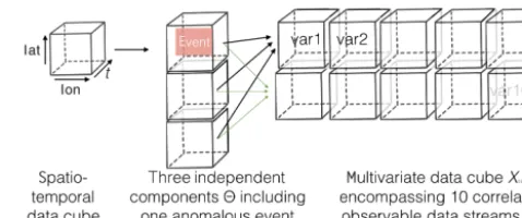
Ground truth for detecting anomalies in multivariate data is rare, in particular for detecting anomalies in real EOs. Thus, we generate artificial data that represent common properties of EOs, including anomalies. In particular, we focus on the existence of seasonality, correlations among variables, and non-Gaussian distributions. Data generation assumes that each subsystem of the Earth has uncorrelated intrinsic prop-erties, i.e., it is dominated by a few independent nents. Consequently, generating these independent compo-nents (which cannot directly be monitored) is the first step. We then derive variables that contain elements of all inde-pendent components and correspond to the observable mea-surements as a set of correlated variables (Fig. 1).
More precisely, as a basic version we create three inde-pendent components for the artificial data, each consisting of a signal (Gaussian, SD=1.0) that includes seasonality in
Figure 1.Combination of three independent component cubes to
derive 10 correlated variablesXas observable measurements. The
anomalous event is propagated into some variables ofX.
some cases (Sect. 2.2). Anomalous events are induced in one of the independent components for which we track the ex-act spatiotemporal location. These three independent com-ponents are then weighted with randomly generated linear (or nonlinear, Sect. 2.3) weights to create a set of 10 corre-lated variables, which represent the artificial data cube, i.e., try to mimic observable measurements. We add some addi-tional measurement noise (Gaussian, SD=0.3) to the data cube. For more technical details of this generation scheme we refer the reader to the Appendix A.
Our standard data cubeXti,j,lat,lon,var encompassesti,j=
1, . . ., T time steps (T =300) corresponding to a 6.5-year time series of satellite images in 8-day intervals, lat=
1, . . ., LAT latitudes (LAT=50), lon=1, . . .,LON longi-tudes (LON=50), and var=1, . . .VAR data streams, or vari-ables (VAR=10).
2.2 Generating anomalous events
Anomalous events are introduced in the independent compo-nents only and then propagated from the independent com-ponent to some of the variables in the data cube with ran-dom weights. The anomalies are contiguous in space and time. The center of the anomaly is assigned randomly. The challenge is to detect the propagated anomaly through the unsupervised algorithms, i.e., without using the information about the spatiotemporal location of the anomaly. With this data cube generation scheme, we can generate anomalies by controlling the type of the anomalous event (event type), the magnitude of the anomalous event, and the spatiotemporal location.
We create four data cubes using the following temporary event types:
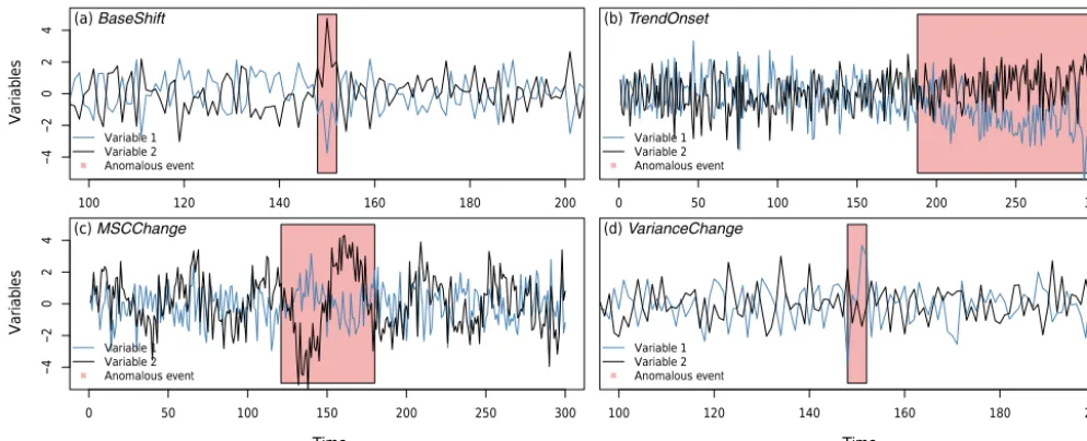
a. a shift in the baseline, i.e., shift of the running mean of a time series (BaseShift) (Fig. 2a). This event type is closely related to extremes in real world EOs.
b. an onset of a trend in the time series (TrendOnset) (Fig. 2b).
100 120 140 160 180 200
Var
iab
les
Variable 1 Variable 2 Anomalous event
(a) BaseShift
Va
ria
bl
es
−4
−2
0
2
4
0 50 100 150 200 250 300
Var
iab
les
Variable 1 Variable 2 Anomalous event
(b) TrendOnset
0 50 100 150 200 250 300
Var
iab
les
Variable 1 Variable 2 Anomalous event
Va
ria
bl
es
Time (c) MSCChange
−4
−2
0
2
4
100 120 140 160 180 200
Var
iab
les
Variable 1 Variable 2 Anomalous event
Time (d) VarianceChange
Figure 2.Visualization of the four different event types(a–d)with two variables along timeti,j=1, . . ., T (T =300). The two variables
contain an anomalous event (red shape) that is propagated through the underlying independent components with randomly drawn weights within the generation process of the variables. For illustration purposes two variables are shown for one specific magnitude of the anomaly. The artificial data farm encompasses 10 variables and anomalous events of 20 different magnitudes ranging from very subtle to exceptionally high changes.
happen in the real world carbon cycle as a response to combined drought–heat waves (Ciais et al., 2005).
d. a change in the variance of the time series (Vari-anceChange) (Fig. 2d), e.g., in temperature (Hunting-ford et al., 2013).
2.3 Additional data properties
Apart from the basic data cubes, we want to test the in-fluence of certain data properties on the anomaly detection algorithm. In order to do so, we create data cubes, each with one added data property, i.e., we increase the num-ber of independent components (MoreIndepComponents) or use a squared dependency among independent components (NonLinearDep) instead of a linear one. Furthermore, typi-cal EO variables are often driven by extrinsic forcings, i.e., the Earth’s solar system orbit, rotation, and axis tilt. Thus, we add a seasonal cycle modifying the signal (SeasonalCycle). In a global context, the mean is rarely constant; we therefore introduce a linear latitudinal trend into the baseline (Latitu-dinalGradient). In the basic case, the signal of our indepen-dent components follows a Gaussian distribution. In the more complicated versions, we also implement alternative scenar-ios with Laplacian (doubly exponentially) distributed signals (LaplacianNoise) and signals that exhibit spatiotemporal cor-relation with red noise (CorrelatedNoise). Signal-to-noise ra-tio is 0.3 in the basic version, one addira-tional data property in-creases the signal-to-noise ratio to 1.0 (NoiseIncrease). Also, the shape and duration of anomalous events differ. We dou-ble (LongExtremes) or reduce the temporal duration of the
anomalous events (ShortExtremes) and change the spatial shape from rectangular to randomly affecting neighboring grid cells (RandomWalkExtreme).
2.4 Experiment design
Each data cube with a specific type of the event is generated 20 times, each time with a different magnitude of the anoma-lous event (Appendix A). We introduce 10 spatially contigu-ous anomalcontigu-ous events into the independent components, with a spatial extent of 20 latitude and longitude steps each. Each event has a temporal extent of five time steps (which would be equivalent to 40 consecutive anomalous days in a 6.5-year record). Our total number of anomalies equals about 3 % of the total data cube, which we consider to be a realistic sce-nario (comparable to Zscheischler et al., 2014a), for example. Some latitudes and longitudes do not exhibit any anomaly by design. The algorithms (Sect. 3.2) are expected to be able to deal with parts of the data cube that do not exhibit anomalies at all, as this is also very likely to happen for applications in real EOs.
Our experiment comprises 36 different event-type combi-nations of data properties, each repeated 20 times with vary-ing event magnitudes (Appendix A). The entire set of artifi-cial data cubes consists of 720 data cubes, corresponding to
≈87 GB of data1.
1Code to reproduce the data farm is provided in the Data
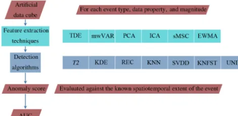
Figure 3.Data processing for detecting multivariate anomalies. We extract relevant features from each artificial data cube before apply-ing the detection algorithms. The detection algorithms output some anomaly score, which we evaluate against the known extent of the event using the area under the curve (AUC). Feature extraction ele-ments on the right-hand side are understood as options and can be combined with each other.
3 Workflows to detect anomalies
The idea of this study is to elaborate workflows that contain both data preprocessing via feature extraction and algorithms for the detection of anomalous events (Fig. 3). In the follow-ing we introduce these two elements separately and explain the performance evaluation strategy afterwards.
3.1 Feature extraction
Feature extraction is a process to derive information from the data and condense it into nonredundant characteristic pat-terns. This may facilitate data interpretation (van der Maaten, 2009). In our study the aim is to maximize the detection of anomalous events by providing relevant features. Feature ex-traction is often an element of data preprocessing. A very simple form of feature extraction could be to subtract the mean seasonal cycle. We consider the anomaly time series to be the extracted feature in this case. Here, we concentrated mainly on feature extraction methods that are used in the con-text of classical multivariate SPC (Lowry and Montgomery, 1995), data-based process monitoring in industry (Ge et al., 2013), and univariate extreme event detection. The following feature extraction methods are used in this study:
Subtracting the median seasonal cycle (sMSC) is one way to deseasonalize time series. Deseasonalization may be in-strumental in detecting anomalous events across different seasons. The remaining part of the time series is often re-ferred to as anomalies in the climatological sense. These anomalies are used here as an input feature. Please note, that the climatological anomalies are only the difference be-tween the mean behavior and thus are not to be mixed up with anomalies (strange or rare regions in the data, closely related to extreme events) as detected through the (multivari-ate) anomaly detection algorithms (Sect. 3.2).
Computing the moving window variance (mwVAR) is a popular technique for detecting trends in the variance in uni-variate time series (e.g., Huntingford et al., 2013). We choose a window size of 10 and compute the variance in the running window along the time series of each variable. We use the estimates of the mwVAR time series as a feature to detect multivariate anomalies in the variance.
Time delay embedding (TDE) increases the feature vector Ytwith time-delayed vectors (Yt=(Xt−0τ,Xt−1τ,Xt− (m−1)τ)) to include temporal context information. In the univariate case, this approach ideally creates an image of the attractor of a dynamical system (Takens, 1980). In high-dimensional multivariate data applications it is used to in-clude information of the dynamics in the feature vector (e.g., Koçak et al., 2004; Ge et al., 2013; Smets et al., 2009). Crit-ical hyperparameters are the time delayτ and the number of dimensionsm. We fixmto 3 (corresponding to the number of independent components within the data farm creation) and
τ to 6, which is a compromise between the typical choice of the first zero crossing of the temporal autocorrelation func-tion or the first local minimum of the mutual informafunc-tion (Webber Jr. and Marwan, 2015) (here: 11.5 corresponding to one-quarter of the annual cycle with 46 time steps) and an accurate temporal detection (requires smallτ).
Principal component analysis (PCA) is a data rotation, used to find an orthogonal (uncorrelated) subspace of the data ofnPC≤VAR variables (Von Storch and Zwiers, 2001). We
choosenPCsuch that at least 95 % of the variance in the
orig-inal data cube is explained. By assuming a homogeneous co-variance structure within the entire data cube, we perform the PCA globally, i.e., with the same rotation matrix for all grid cells. The combination of TDE and PCA is sometimes re-ferred to as dynamic PCA when considering subsequent lags in the time series (Lee et al., 2004).
Independent component analysis (ICA) can be regarded as a nonlinear alternative to PCA; it has become a standard technique of data-based process monitoring. We use one ICA variant that tries to separate different sources of data by max-imizing the negentropy, a measure of non-Gaussianity of the data (Hyväringen and Oja, 2000)2. We apply ICA globally to each data cube. The hyperparameter is the number of in-dependent components (sources). We choose the number of independent components to be equal tonPC (see PCA) for
consistency reasons (Majeed and Avison, 2014).
Exponentially weighted moving average (EWMA) is one way of reducing the noise of the time series and taking tem-poral information into account. It is common in the context of classical multivariate SPC to detect only “significant” out-liers (Lowry and Woodall, 1992). The multivariate feature time seriesYis computed recursively as
Yti=λXti+(1−λ)Yti−1. (1)
2We use the fastICA algorithm implemented in the
ju-lia package MultivariateStats.jl (https://github.com/JuliaStats/
The hyperparameter λ determines the degree of exponen-tial weighting between 1 (no weighting) and zero (common choice 0.1≤λ≤0.3; Santos-Fernández, 2013). We stay in this range withλ=0.15.
There is of course a multitude of alternative approaches available in the literature, but we focus on the previously summarized ones as they are widely used and efficiently im-plemented. Furthermore, different feature extraction meth-ods can also be combined (Fig. 3). As the number of pos-sible combinations is considerably large, we focus here on dimensionality reduction techniques (ICA, PCA) combined with some EWMA to reduce the noise level afterwards. De-pending on the event type and data properties, additionally removing seasonality (sMSC) or including the variance mw-VAR seems to be straightforward. Information about the dynamics (TDE) can be included before applying dimen-sionality reduction techniques to keep the dimendimen-sionality of the system as low as possible. In the following, combi-nations are noted in the order in which they were applied (e.g., PCA_EWMA means first applying PCA, then applying EWMA to the PCA features). In some cases this might lead to non-commutative combinations, especially for nonlinear feature extraction techniques (ICA, TDE).
3.2 Anomaly detection algorithms
We use several detection algorithms that we implemented in the Julia package MultivariateAnomalies (https://github. com/milanflach/MultivariateAnomalies.jl). Some anomaly detection algorithms require the estimation of parameters (details are given below for each algorithm separately). In that case we fix the model parameters for the entire data cube. We estimate model parameters (σ,ε,Q,µ; see below) and train the models themselves (support vector data description, kernel Null Foley–Sammon Transform, KNFST; see below) based on a random subsample of 5000 data points obtained from the entire data cube. To account for variability in the model parameter estimation, we resample three times. More resampling is not affordable due to high computational costs of processing the large number of data cubes. However, very little random variability is observed with this sample size for the best algorithms. Thus, we consider a resampling of three times to be sufficient for a first attempt to account for vari-ability in the parameterization. The following algorithms are investigated for anomaly detection.
Univariate approach (UNIV) is a simple approach to de-fine extremes in univariate data by identifying all points above (or below) a certain quantile. This so-called “peak-over-threshold” approach can be transferred to deal with mul-tiple univariate data streams. In this case, one would con-sider a data point to be extreme if one or several of the univariate variables are above (or below) a certain quantile threshold of the marginal distributions of each single vari-able. (here: globally) (e.g., Ledford and Tawn, 1996; Bae et al., 2003; Donges et al., 2016). Applications of the
so-called co-occurrence or coincidence analysis can be found in Donges et al. (2011b), Rammig et al. (2015), Zscheischler et al. (2015), Guanche et al. (2016), and Siegmund et al. (2016). For comparing the algorithms, we are interested in the information that at least one variable is above a certain threshold. We compute this information for different thresh-olds (in terms of quantiles of the marginal distributions be-tween 0.0 and 1.0, accuracy 0.01) to get a score, i.e., a rank-ing of the extremeness of the data points.
Hotelling’s T2 (T2) computes the squared Mahalanobis distance of each data point Xt to its temporal mean µ weighted with the covariance matrixQ(Hotelling, 1947):
(Xt−µ)0Q−1(Xt−µ). (2)
A crucial prerequisite is the estimation of the covariance matrix Q, which is estimated from the random subsam-ple of 5000 data points. Combining the feature extraction EWMA withT2 equals the traditional multivariate exponen-tial weighted moving average (Lowry and Woodall, 1992; Lowry and Montgomery, 1995).
Apart from computing weighted distances to the mean (likeT2), it is also possible to compute pairwise Euclidean distances in variable spaced(Xti,Xtj) between vectorsXti
andXtj of time stepsti andtj for all possible time steps
ti, tj=1. . .T. The resulting matrixDwithDij=d(Xti,Xtj)
is often referred to as distance matrix or dissimilarity matrix. For real world data, variables have to be standardized with care before computing the distance matrix (Sect. 5). How-ever, in the artificial data used the variables are already com-parable by construction; thus, standardization is not needed. The following algorithms are based on pairwise distances.
K-nearest neighbors (KNNs) can be used for anomaly de-tection by considering the mean distance to the k-nearest neighbors (k-nearest neighbors Gamma, KNN-Gamma) and the length of the mean of the vectors pointing fromXti to its
k-nearest neighbors (k-nearest neighbors Delta, KNN-Delta) (Harmeling et al., 2006; Ramaswamy et al., 2000). With the latter approach KNN-Delta also considers the direction of the neighbors, i.e., has higher values in case its nearest neigh-bors are pointing in one direction, which is in contrast to the directionless distance of KNN-Gamma. We fix the hyperpa-rameterk at 10 after carefully trying different choices for
k without seeing major effects on preliminary results. Fur-thermore, we exclude trivial temporal autocorrelations by ex-cluding five neighboring time steps (abs(ti−tj)≥5) to also be nearest neighbors.
rare or unusual. Faranda and Vaienti (2013) used the concept of recurrences and combined it with extreme value theory. We want to use a more general approach without binning the time series. We count the number of observations ζ falling into a certainεball in a system of multiple variables, con-densed by their distanced(Xti,Xtj):
ζ(Xti)=
T X
j=1
8(ε−d(Xti,Xtj)). (3)
8(z) is the Heaviside function, coding the distances to binary values (8(z)=0 ifz <0,8(z)=1 otherwise). Anε hyper-ball containing only few recurrent observations is considered to be rare in comparison to the majority ofζ values. We com-pute 1−ζ·T−1to get anomaly scores, which are more likely to be an anomaly for high score values.ζ·T−1is known as local recurrence rate or degree density in recurrence analy-sis (Marwan et al., 2007; Donner et al., 2010) (Donges et al., 2012).εis the crucial hyperparameter, defining the radius of the ball. Typical choices ofεin recurrence analysis are quan-tiles of the distribution of elements of the distance matrix, e.g., 5 or 10 % (Donges et al., 2011a; Flach et al., 2016). As we are not interested in small-scale variations in REC, but more in major anomalies we estimateεas median of the dis-tance matrices in the random subsample. This choice turned out to be the optimal choice (in terms of maximizing the area under the curve, AUC; Sect. 3.3) forεin a small simulation, varying the thresholds between the 5 and 95 % quantiles of the element of the distance matrix (Supplement Fig. S1). We exclude five neighboring time steps to be counted as recur-rences (similar to KNN). KNN has similarities to REC, as one could also choose a data-adaptiveksuch thatζ =k.
The distance matrix D can be transformed into a kernel matrixK=exp(−0.5·D·σ−2), i.e., by computing pairwise dissimilarities using Gaussian kernels centered on each data point.
Kernel density estimation (KDE) is a standard technique for estimating densities based on column means of the kernel matrixK (Parzen, 1962). The bandwidthσ of the kernel is a hyperparameter. We estimateσby using the median of the temporal distance matrix on the random subsample, which is a common choice (Schölkopf and Smola, 2001; Schölkopf et al., 2015).
Support vector data description (SVDD) models the distri-bution of the training data with an enclosing hypersphere in a high-dimensional kernel feature space (Tax and Duin, 2004). As usual a kernel matrix of the random subsample is used for training. Although being a rather simple data description, a hypersphere in the kernel feature space can result in com-plex nonlinear decision boundaries in the original space of predictor variables if a nonlinear kernel function is used. In addition to theσ hyperparameter of the kernel function (see KDE), the SVDD approach has a parameter called outlier ra-tioν (fixed to 0.2). The outlier ratioν controls the number of training samples that can be located outside of the
hyper-sphere to prevent overfitting. As anomaly score for testing, its distance to the center of the hypersphere in the kernel fea-ture space is computed. Testing requires pairwise similarities between test and training samples. For performance reasons in terms of computation time, we used the implementation by (Chang and Lin, 2013) of the one-class support vector machine (Schölkopf et al., 2001), which is an alternative for-mulation that leads to identical data descriptions as SVDD in our setup.
kernel Null Foley–Sammon Transform (KNFST) maps the training data into a so-called null space, in which the train-ing samples have zero variance, i.e., all traintrain-ing samples are mapped to the same point called the target value (Bodesheim et al., 2013). Nonlinearity is incorporated by using a kernel matrix containing pairwise similarities of the training sam-ples (training on the random subsample as for SVDD). Since all training samples are represented by a single target value in the one-dimensional null space, the anomaly score of a test sample is the absolute difference between its projection in the null space and this target value. The projection of the test sample requires pairwise similarities to the training samples. Compared to SVDD no parameters need to be tuned except forσ of the kernel function that is fixed to the same values for all kernel methods.
3.3 Ranking of the workflows
Given the large number of potential combinations of fea-ture extraction and anomaly detection algorithms, we need an objective criterion to compare the performances of the numerous possible workflows. We use the area under the re-ceiver operator characteristics curve (AUC) as our measure of detection skill for a specific event type (Fawcett, 2006). The AUC is based on the fraction of events that are cor-rectly detected (true positives) and the fraction of detections among all non-events (false positives), for all possible de-cision thresholds that could be applied to scores produced by the algorithms. AUC values of 0.5 would be achieved by random detection, and values below 0.5 indicate that a lower score is more likely assigned to (true) anomalies than to non-anomalies.
the Arctic due to abrupt sea ice losses (Bintanja and van der Linden, 2013; Bathiany et al., 2016), for example) or an in-crease in the signal variance of 25 % (e.g., in temperature; Huntingford et al., 2013).
One way of summarizing the results of such a large num-ber of combinations is treating the AUC values as the out-comes of an experiment in which the different design deci-sions (e.g., feature extraction techniques, anomaly detection algorithms) are the experimental factors. As a control treat-ment we introduce the simplest possible approach to detect-ing the anomaly: UNIV approach on the selected event type, without any further data properties (e.g., short extremes or increased measurement noise) on the event type and without prior feature extraction. In order to assess the (averaged) ef-fect of each experimental factor, we fit a linear mixed-efef-fect model (Pinheiro et al., 2016) to the AUC data (fixed effects: data properties, feature extraction, anomaly detection algo-rithms; random effect: magnitude of the event). This model’s coefficients express the overall effect of a factor level with respect to the control while averaging over all other exper-imental factors. They are considered to be significant for
p <0.01.
Additionally, we compute the resampling variation in parameter estimation of the anomaly detection algorithms (RVP) as mean difference of the maximum AUC and min-imum AUC for each resamplingi=1. . .3 (Sect. 3.2).
RVPalgorithm=mean(max(AUCcomp,feat,magn,event,i)
−min(AUCcomp,feat,magn,event,i)) (4)
3.4 Ensembles of anomaly detection algorithms
Summarizing the output of several anomaly detection algo-rithms is one way to create more robust results (Thompson, 1977). For better comparability of the algorithms’ outputs, we rank them by computing the percentiles of the algorithm scores. These are then aggregated into ensemble scores by computing the minimum (consensus voting), the mean (bal-anced voting), or the maximum (risky voting) of the scores of selected well-performing algorithms (e.g., Aggarwal, 2012; Zimek et al., 2013).
4 Results and discussion
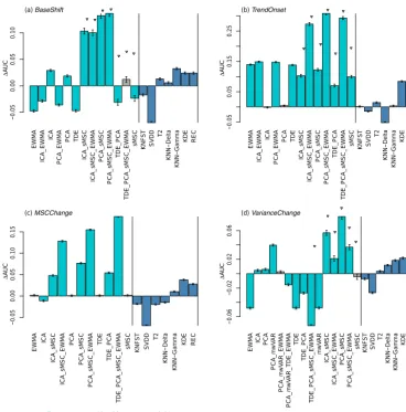
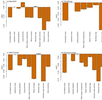
In the following, we present the performance of the work-flows in subsections corresponding to feature extraction tech-niques (Sect. 4.1), anomaly detection algorithms (Sect. 4.2), and ensembles of detection algorithms (Sect. 4.3). Specifi-cally, we present the AUC difference to the UNIV control, i.e., the output of the linear mixed-effect model on the ex-perimental factors feature extraction and detection algorithm (Fig. 4). The corresponding tables present the estimates as well as the RVP (Tables 1, 2). Apart from the model the full range of AUC values with respect to different event
magni-tudes, data properties, and event types is presented in Ap-pendix B, Fig. B1.
4.1 Feature extraction techniques
Feature extraction techniques are often more important than the detection algorithm itself (Fig. 4). However, we find that choosing a suitable feature extraction technique largely de-pends on the event type of interest. Therefore, the feature extraction techniques are presented for different event types separately.
BaseShift Shifts in the baseline are simulated to mimic ex-treme events. Increasing the magnitude (in terms of standard deviations) of a BaseShift makes it easier to de-tect the event (Fig. B1). Dimensionality reduction (via PCA or ICA) is a crucial feature extraction technique step as it derives meaningful uncorrelated subsets of the data (Fig. 4a). The combination of dimensionality re-duction with some temporal smoothing (EWMA) does not exhibit better overall performance (Fig. 4a) as it fails for ShortExtremes due to oversmoothing. Never-theless, EWMA can improve the detection rate for spe-cial cases, i.e., long events (LongExtremes) and high signal-to-noise ratios (NoiseIncrease) (Fig. B1).
TrendOnset Results look very similar to those of Base-Shift, except that temporal smoothing with EWMA has a stronger positive effect than for BaseShift. This may be related to the fact that events for TrendOnset are longer than those for BaseShift. Since the algorithms used in this work are not specifically designed to detect the onset of linear trends, we speculate that their capa-bility to detect such anomalies may be related to their ability to detect base shifts. While algorithms specifi-cally designed to detect changes in trends (e.g., Forkel et al., 2013)) were not included in our work due to our focus on more generic types of anomalies, such special-ized algorithms may perform better for this particular class of anomaly.
EWMA
ICA_EWMA
ICA
PCA_EWMA
PCA TDE
ICA_sMSC
ICA_sMSC_EWMA
PCA_sMSC
PCA_sMSC_EWMA
TDE_PCA
TDE_PCA_sMSC_EWMA
sMSC KNFST SVDD
T2
KNN−Delta
KNN−Gamma
KDE REC
−0.05
0.00
0.05
0.10
∆
A
UC
(a) BaseShift
EWMA
ICA_EWMA
ICA
PCA_EWMA
PCA TDE
ICA_sMSC
ICA_sMSC_EWMA
PCA_sMSC
PCA_sMSC_EWMA
TDE_PCA
TDE_PCA_sMSC_EWMA
sMSC KNFST SVDD
T2
KNN−Delta
KNN−Gamma
KDE REC
−0.05
0.05
0.15
0.25
∆
A
UC
(b) TrendOnset
EWMA
ICA
ICA_sMSC
ICA_sMSC_EWMA
PCA
PCA_sMSC
PCA_sMSC_EWMA
TDE
TDE_PCA
TDE_PCA_sMSC_EWMA
sMSC KNFST SVDD
T2
KNN−Delta
KNN−Gamma
KDE REC
−0.05
0.00
0.05
0.10
0.15
∆
A
UC
(c) MSCChange
EWMA
ICA PCA
PCA_mwV
AR
PCA_mwV
AR_EWMA
PCA_mwV
AR_TDE_EWMA
TDE
TDE_PCA
TDE_PCA_sMSC_EWMA
mwV
AR
ICA_sMSC
ICA_sMSC_EWMA
PCA_sMSC
PCA_sMSC_EWMA
sMSC KNFST SVDD
T2
KNN−Delta
KNN−Gamma
KDE REC
−0.06
−0.02
0.02
0.06
∆
A
UC
(d) VarianceChange
Only applied for data with SeasonalCycle
Feature extr Algorithm p > 0.01
Figure 4.AUC difference with respect to the UNIV control in the experimental factors feature extraction and detection algorithm for the
event types(a–d).
VarianceChange The algorithms used are hardly able to de-tect any decrease in variance (Fig. B1). This may be due to an overwriting of the decrease in signal vari-ance with the independent noise since we are using a signal-to-noise ratio of 0.3. Thus, we exclude a decrease in the variance from the evaluation of the detection al-gorithms compared to the control. The detection of an increase in the variance can be improved by a combina-tion of dimensionality reduccombina-tion and variance in a mov-ing window (PCA_mwVAR) (Fig. 4d). Usmov-ing the vari-ance in a moving window is a popular approach (Hunt-ingford et al., 2013) although it has to be applied with care when used in conjunction with normalization pro-cedures (Sippel et al., 2015).
SeasonalCycle Seasonality occurs in most EOs. Not ac-counting for the seasonal cycle has a negative impact on the AUC (Appendix B, Fig. B2a, b, d). However, if we subtract the median cycle within the feature
ex-traction step (PCA_sMSC_EWMA; Fig. 4a, b, d), we can almost account for the negative AUC impact of the seasonal cycle, as in our experimental setting anoma-lous events do occur independently of seasonality. How-ever, depending on the research question, independence of seasonality might not always be the case: some EOs may depend on vegetation activity, for example, which results in a strong dependence on seasonality.
4.2 Performance of multivariate anomaly detection algorithms
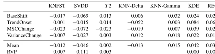
Table 1.Average AUC difference of the anomaly detection algorithms from the UNIV control for each event type.
KNFST SVDD T2 KNN-Delta KNN-Gamma KDE REC
BaseShift −0.017 −0.069 0.013 0.006 0.032 0.024 0.024
TrendOnset 0.001 −0.015 0.014 −0.052 0.003 0.084 0.068
MSCChange −0.023 −0.072 −0.023 −0.019 0.007 0.039 0.029
VarianceChange −0.007 −0.027 0.003 0.012 0.018 0.022 0.019
Mean −0.012 −0.046 0.002 −0.013 0.015 0.042 0.035
RVP 0.007 0.111 0.003 0.000 0.001
KDE and REC These techniques exhibit overall the high-est AUC and lowhigh-est RVP (Table 1). Their high-estimated mean differences are rather small since REC can be con-sidered as a binary form of the KDE. As REC uses a threshold ε for defining the hyperball of recurrences, the results can exhibit slightly higher AUC than KDE (Fig. S1). However, with REC the caveat is that the pa-rameterεis not necessarily optimally chosen.
KNN In most of the cases, KNN-Gamma performance is better than the UNIV control, but only as good as the UNIV control for detecting TrendOnset. This may be due to the fact that for TrendOnset, the mean distance to the KNN does not change, unless considering a very large number of KNN values or excluding a large frac-tion of temporally near data points to be within the KNN. When excluding TrendOnset, the mean perfor-mance increases to 0.019, which is comparable to KDE and REC. In addition, we observe even superior perfor-mance of KNN-Gamma compared to KDE and REC for difficult data properties (e.g., MoreIndepComponents, CorrelatedNoise; Fig. S2). In contrast, KNN-Delta does not yield high AUC, probably because we do not con-struct anomalies in the data cube explicitly with a direc-tion that is accounted for by KNN-Delta (mean length of the vectors to its KNN). The finding that simple algo-rithms like KNN-Gamma (or KDE,T2) are very com-petitive, if not favorable algorithms, is in line with re-sults of Harmeling et al. (2006), Killourhy and Maxion (2009), and Ding et al. (2014) for various data sets.
KNFST and SVDD These techniques perform on average worse than or equally as well as UNIV. Also, the RVP is highest among the algorithms (Table 1). It has al-ready been reported that SVDD can exhibit remarkable fluctuations in the results for sample sizes smaller than 1000 data points (Ding et al., 2014). However, we use 5000 points for training. Thus, we suggest that the fluc-tuations are due to the fact that SVDD and KNFST use a training set that is chosen at random and may it-self contain anomalies. In the current setting the size of the training sample (5000) is rather small compared to the spatiotemporal size of the data cube (750 000), and it does not seem to be sufficient to train these
algo-rithms on the data cube. Increased sample sizes, how-ever, would heavily increase memory demand and com-puting time, rendering kernel algorithms computation-ally inapplicable. Furthermore, Ding et al. (2014) shows that the sample size has a remarkable effect for SVDD (better performance for lager sample sizes). However, even with very large sample sizes SVDD still performs worse than KNN in the setting of Ding et al. Train-ing and testTrain-ing SVDD on each pixel does also not im-prove the results as the number of anomalies differs be-tween different pixels in our setting. Training and test-ing SVDD on each pixel assumes the same number of anomalies in each pixel (constant outlier ratio assumed by the fixedνparameter), which is contrary to the gen-eration of the artificial data farm.
We explicitly do not want to state that KNFST and SVDD are generally worse algorithms, i.e., they are just not built for these massive numbers of data. KNFST and SVDD outperform other algorithms in very differ-ent settings (novelty detection in images) (Bodesheim et al., 2013).
−0.10
0.05
Time [yr]
sMSC (Fpar)
2001 2004 2007 2010
(a)
−0.5
1.0
Time [yr]
sMSC (GPP)
2001 2004 2007 2010
(b)
Figure 5. The residual time series obtained by subtracting the median seasonal cycle from(a)the fraction of absorbed photosynthetic
radiation (fPAR) and(b)gross primary productivity (GPP) at northern latitudes exhibit heteroscedastic patterns.
4.3 Ensembles
The selection of algorithms for computing the ensemble is a compromise between accurate detection of and diversity amongst the selected algorithms (Zimek et al., 2013). We se-lect the four best algorithms (KDE, REC, KNN-Gamma,T2; referred to together as 4b) and the three best distance-based algorithms (KDE, REC, KNN-Gamma; referred to together as 3d) for computing their ensembles. We assume that this choice accounts for accuracy (best algorithms selected) as well as for diversity (different algorithms selected).
Overall, ensemble building improves the anomaly detec-tion rate. The mean AUC of each of the ensemble members (3d:+0.030, 4b:+0.023) is lower than the AUC of the en-semble, regardless of whether the maximum or the mean is used for ensemble aggregation. Minimum aggregation of en-semble members, however, performs worse than the individ-ual ensemble members REC and KDE. Using the maximum or mean yields consistently higher AUC than using the min-imum (Table 2). The superior performance of the maxmin-imum choice compared to the minimum indicates that single al-gorithms overlook more often anomalous events than rais-ing false alarm. Nevertheless, the maximum has the caveat that even a single algorithm may cause a false alarm (Zimek et al., 2013), e.g., due to a poor parameterization or inade-quate assumptions about properties of the data. Thus, a more balanced voting procedure like the mean is the preferable choice and more stable with respect to possible error sources. Among the mean ensembles, the 3d or 4b ensembles perform equally well (0.041 vs. 0.039±0.001 overall) (Table 2).
4.4 Limitations
High dimensionality The utility of distance-based outlier detection algorithms as used in this paper is often ques-tioned in the context of high-dimensional data (Zimek et al., 2012). The “curse of dimensionality” states that the difference between near and far distances diminishes with increasing dimensionality. However, Zimek et al. (2012) showed in the case of KNN that the contrary is true for outliers with fixed magnitude in otherwise un-correlated data. Dimensionality reduction as crucial fea-ture extraction transforms the data into a few (ideally)
meaningful and uncorrelated variables. Thus, the find-ings of Zimek et al. (2012) provide strong arguments for applying dimensionality reduction on correlated data. We anticipate that their findings are the reason of the superior performance of dimensionality reduction here.
Heuristic choices Within the parameterization process, sev-eral heuristic choices are made. We exclude five time steps to be counted as recurrences ork-nearest neigh-bors. We fix several parameters, e.g., the number of nearest neighbors is fixed to 10. Also, other parame-ter choices are rather heuristic (e.g.,σ), although com-monly used. The artificial data farm’s intrinsic dimen-sion is 3 as it was created from three independent com-ponents. Therefore, the embedding dimensionmis fixed accordingly, although it can be inferred based on the data by determining the number of false nearest neigh-bors (Kennel et al., 1992; Hegger et al., 1999). The signal-to-noise ratio of our artificial data farm is 0.3. Furthermore, the choice of the data properties might influence the results for each event type, as the stan-dard deviation of AUC values over all data properties (0.05) is rather large, compared to the average AUC gain of the three best algorithms with respect to the control (+0.03). However, the ordering of the algorithms is also important to derive rankings of algorithms (Hornik and Meyer, 2007). By choosing different subsets of the data properties, we observe that the three best algorithms (KDE, REC, KNN-Gamma) are on top, independently of the chosen data property. Therefore, the data proper-ties might have an influence on the AUC values them-selves, but not on the choice of the top three candidates.
5 Remarks on applications for real Earth observations
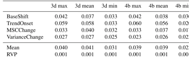
Table 2.AUC difference of the ensembles of anomaly detection algorithms to the UNIV control. Ensembles are computed out of the four
best algorithms (4b, KDE, REC, KNN-Gamma,T2) and the three best distance-based algorithms (3d, KDE, REC, KNN-Gamma).
3d max 3d mean 3d min 4b max 4b mean 4b min
BaseShift 0.042 0.037 0.033 0.042 0.038 0.030
TrendOnset 0.059 0.058 0.033 0.060 0.056 0.020
MSCChange 0.033 0.040 0.032 0.033 0.037 0.017
VarianceChange 0.027 0.027 0.025 0.023 0.026 0.022
Mean 0.040 0.041 0.031 0.039 0.039 0.022
RVP 0.001 0.001 0.001 0.001 0.001 0.001
A typical preprocessing of EOs is to center variables to zero mean and standardize to unit variance (also known as
z transformation). A standardization of this kind is of key importance in global EOs. Real multivariate observations of-ten have different physical units or ranges, which have to be made comparable before analyzing. However, standard-ization has to be applied with care. Differences between the mean and variance between geographically distinct or even adjacent grid cells as well as seasonal cycles might corrupt any further analysis. We recommend subtracting the median seasonal cycle before standardization. The median is pre-ferred over the mean as mean seasonal cycles are affected by changes in the amplitude of the cycle. Standardization can be applied globally (i.e., with global spatiotemporal mean and variance), regionally (i.e., with spatiotemporal mean and variance in subregions of the globe), or locally (i.e., with temporal mean and variance in each grid cell). Global stan-dardization might be more robust than local but detects only anomalies in high-variance regions. Local standardization as-sumes that the number of extreme anomalies is equal in each grid cell, which is a rather strong assumption. Thus, a re-gional standardization is favorable in regions with similar mean and variance.
Especially variables presenting a signal from the biosphere are known to exhibit heteroscedasticity, e.g., the variance during growing season is substantially larger than during the rest of the year (Fig. 5). Atmospheric variables in high latitudes also show higher variability during the cold sea-son, e.g., temperature variability might be higher over ice (cold season) than over open water (warm season) (Hansen et al., 2012). Specifically for global applications, using es-timates of variance or standard deviation locally (in each grid cell) leads to an underestimation of the variance during growing season and thus to an overestimation of anomalies due to standardization, especially in the northern latitudes (Guanche et al., 2016). Thus, we recommend accounting for the heteroscedastic pattern by adjusting the variance during the growing season within similar regions. We also recom-mend this kind of adjustment for the covariance matrix used, e.g., inT2 or PCA as well as for the parameterization of KDE or REC.
Furthermore, anomalies are also overestimated when us-ing a reference period for the estimation of the variance (Sip-pel et al., 2015). However, with 300 observations in 8-day intervals, as used in this study, this issue is expected to be less pronounced than for fewer observations as it scales with the length of the time series. Nevertheless, we rather recom-mend using estimates of the variance of the entire time series or correcting for the overestimation in the out-of-reference period as shown in Sippel et al. (2015).
Regarding the parameterization process of the algorithms, we use fixed parameters forσ,ε,k,ν, mean vector, and co-variance matrix globally on the entire artificial data cube. Local parameterization assumes the same number of anoma-lies in each region, which is neither suitable for the artificial data by construction nor for real global data. Thus, we rec-ommend parameterizing globally or within similar regions. Classification of the Earth into similar regions and applying multivariate extreme detection in each region will be the sub-ject of future research.
6 Conclusions
Our aim is to identify suitable methods for detecting anoma-lies in highly multivariate, correlated, and seasonally varying data streams as they are common in Earth system science. In particular, we are interested in detecting shifts in mean (extremes), changes in the amplitude of the seasonal cycle, temporal changes in the variance, and onsets of trends. We test a wide range of workflows (i.e., combining feature ex-traction techniques and anomaly detection algorithms). All experiments are based on artificial data, designed to mimic real world Earth observations.
We can show that, on average over different anomaly types and data properties, three multivariate anomaly detec-tion algorithms (KDE, REC, KNN-Gamma) outperform uni-variate extreme event detection as well as other multivari-ate approaches (mean AUC compared to univarimultivari-ate control:
However, we also find for the considered type of events that including a suitable feature extraction technique in the detection workflow is often more important than the choice of the event detection algorithm itself. However, we find that the feature extraction has to be explicitly designed for the event type of interest, i.e., time delay embedding (for detecting changes in the cycle amplitude) and exponential weighted moving average (for detecting trends and long ex-tremes and removing uncorrelated noise in the signal) in-creases the detection rate of the anomalous events. Includ-ing features of the variance within a movInclud-ing window works partly for detecting increases in the variance but fails to de-tect a decrease in the variance due to the relatively high ob-servational noise level. In general, if the data comprise sea-sonality, subtracting them and using the remaining time se-ries as the input feature is essential. Furthermore, we im-prove the detection rate of multivariate anomalies in highly correlated data streams by adding a dimensionality reduction method to the workflow (in line with results of Zimek et al., 2012).
The proposed workflows are capable of dealing with com-mon properties of Earth observations like seasonality, non-linear dependencies, and (to a certain degree) non-Gaussian distributions and noise. Nevertheless, they have to be applied with care to Earth observations, i.e., standardization issues along with strong heteroscedastic patterns (e.g., in biosphere variables of northern latitudes) may lead to an overestima-tion of anomalies. Future work will explore the potential of the identified workflows in rediscovering known and poten-tially unknown extremes as well as other anomalies in a set of real Earth system science data streams. We anticipate that an automated application of our workflows might enable the establishment of automated Earth system process control in a very generic manner.
Appendix A: Technical details on generating the artificial data
Within the generation process, we assume that the signalS
is additive to the baseline B. The baseline might represent reoccurring patterns like seasonality or a constant mean. In addition, binary event parameters evt,lat,lon are introduced,
which allow for switching the anomaly on (evt,lat,lon6=0)
and off (evt,lat,lon=0) (normality). The event type and
mag-nitude of the event is controlled separately by a parameter for the baseline (kb), the signal (ks), and a mean-shift parameter
(km) scaled with the standard deviation of the data (SD).
2t,lat,lon=Bt,lat,lon·2(kb·evt,lat,lon)+St,lat,lon·2(ks·evt,lat,lon)
+km·evt,lat,lon·SD (A1)
For a basic version, three independent components
2t,lat,lon,varare created with the signal consisting of Gaussian
noise (SD=1). Each component represents intrinsic proper-ties of the Earth system. Furthermore, we assume that prop-erties of the Earth system2t,lat,lonare not measured directly
but indirectly via a set of correlated variables, i.e., represent-ing patterns of these intrinsic properties. Hence, these vari-ables propagate anomalous events that occur in one indepen-dent component. This set of correlated variablesXvaris
cre-ated by weighting the intrinsic properties2varwith randomly
drawn linear (or nonlinear) weightswj plus additional mea-surement noise (Gaussian, SD=0.3) added to each vari-able.
Xvar=
j=3
X
j=1
wj·2j+ (A2)
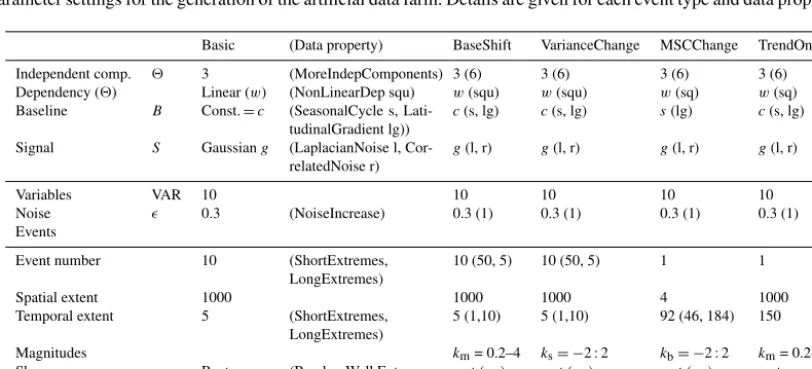
Table A1.Parameter settings for the generation of the artificial data farm. Details are given for each event type and data property (in brackets).
Basic (Data property) BaseShift VarianceChange MSCChange TrendOnset
Independent comp. 2 3 (MoreIndepComponents) 3 (6) 3 (6) 3 (6) 3 (6)
Dependency (2) Linear (w) (NonLinearDep squ) w(squ) w(squ) w(sq) w(sq)
Baseline B Const.=c (SeasonalCycle s,
Lati-tudinalGradient lg))
c(s, lg) c(s, lg) s(lg) c(s, lg)
Signal S Gaussiang (LaplacianNoise l,
Cor-relatedNoise r)
g(l, r) g(l, r) g(l, r) g(l, r)
Variables VAR 10 10 10 10 10
Noise 0.3 (NoiseIncrease) 0.3 (1) 0.3 (1) 0.3 (1) 0.3 (1)
Events
Event number 10 (ShortExtremes,
LongExtremes)
10 (50, 5) 10 (50, 5) 1 1
Spatial extent 1000 1000 1000 4 1000
Temporal extent 5 (ShortExtremes,
LongExtremes)
5 (1,10) 5 (1,10) 92 (46, 184) 150
Magnitudes km= 0.2–4 ks= −2 : 2 kb= −2 : 2 km= 0.2-4
Shape Rect. (RandomWalkExtreme
rw)
rect (rw) rect (rw) rect (rw) rect
Using this data generation scheme, a standard data cube Xti,j,lat,lon,var is created, encompassing 300 time steps (T),
10 temporally correlated variables (VAR), and the total num-ber of latitudes (LAT) and longitudes (LON) fixed to 50 each. We induce anomalous events with a spatial extent of 40 % of the latitude and longitude and 10 events, each with a tempo-ral extent of five time steps. Our total number of anomalies equals about 3 % of the total data cube.
In the basic version we create four data cubes, each with a different temporary event type, including
– shift in the baseline, i.e., shift of the running mean of a time series (BaseShift) (Fig. 2a);
– change in the variance of the time series (Vari-anceChange) (Fig. 2b);
– change in the amplitude of the mean seasonal cycle of a time series (MSCChange) (Fig. 2c);
– onset of a trend in the time series (TrendOnset) (Fig. 2d).
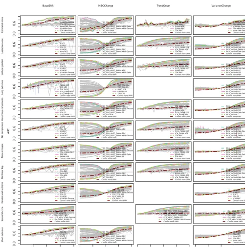
Appendix B: Detailed results ICA KNN−Gamma PCA KNN−Gamma None KNN−Gamma ICA KNN−Delta PCA KNN−Delta Control: none UNIV
0.0 0.6 Correlated noise BaseShift TDE_PCA KDE TDE_PCA REC TDE_PCA_sMSC_EWMA KNN−Delta TDE_PCA_sMSC_EWMA KNN−Gamma TDE_PCA UNIV
Control: none UNIV MSCChange ICA_EWMA KDE TDE KDE EWMA KDE EWMA REC TDE REC Control: none UNIV TrendOnset ICA KNN−Delta PCA KNN−Delta ICA KNN−Gamma PCA KNN−Gamma None KNN−Delta Control: none UNIV VarianceChange ICA T2 ICA REC PCA T2 ICA KDE None REC Control: none UNIV
0.0 0.6 Laplacian noise TDE_PCA KDE TDE_PCA_sMSC_EWMA KDE TDE_PCA REC TDE_PCA_sMSC_EWMA REC TDE_PCA_sMSC_EWMA KNN−Gamma Control: none UNIV
TDE KDE EWMA KDE PCA_EWMA KDE ICA_EWMA KDE TDE REC Control: none UNIV
PCA_mwVAR KDE PCA_mwVAR REC PCA_mwVAR KNN−Gamma PCA_mwVAR_EWMA KDE PCA_mwVAR KNN−Delta Control: none UNIV
ICA T2 PCA T2 ICA REC ICA KDE ICA KNN−Gamma Control: none UNIV
0.0 0.6 La tit ud e gr ad ie nt TDE_PCA_sMSC_EWMA REC TDE_PCA_sMSC_EWMA KNN−Gamma TDE_PCA KDE TDE_PCA_sMSC_EWMA KDE TDE_PCA_sMSC_EWMA KNN−Delta Control: none UNIV
ICA_EWMA KDE ICA_EWMA REC PCA_EWMA REC EWMA REC TDE REC Control: none UNIV
PCA_mwVAR KNN−Gamma PCA_mwVAR T2 PCA_mwVAR KNN−Delta PCA_mwVAR REC PCA_mwVAR KDE Control: none UNIV
EWMA KDE TDE KDE TDE SVDD PCA_EWMA KDE ICA_EWMA KDE Control: none UNIV
0.0 0.6 Lo ng e xt re m es TDE_PCA KDE TDE_PCA REC sMSC KDE EWMA KDE TDE KDE Control: none UNIV
PCA_mwVAR T2 PCA_mwVAR KDE PCA_mwVAR KNN−Gamma PCA_mwVAR REC PCA_mwVAR KNN−Delta Control: none UNIV
ICA_EWMA KDE ICA_EWMA REC ICA T2 PCA T2 ICA_EWMA T2 Control: none UNIV
0.0 0.6 M or e in de p co m po ne nt s TDE_PCA_sMSC_EWMA KDE TDE_PCA_sMSC_EWMA KNN−Gamma TDE_PCA_sMSC_EWMA REC TDE_PCA_sMSC_EWMA T2 TDE_PCA KDE Control: none UNIV
ICA_EWMA KDE TDE KDE EWMA KDE PCA_EWMA KDE ICA_EWMA REC Control: none UNIV
PCA_mwVAR KNN−Gamma PCA_mwVAR REC PCA_mwVAR KDE PCA_mwVAR KNN−Delta PCA_mwVAR T2 Control: none UNIV
ICA T2 PCA T2 ICA REC ICA KDE None REC Control: none UNIV
0.0 0.6 N o co m pl ic at io n TDE_PCA KDE TDE_PCA_sMSC_EWMA KDE TDE_PCA REC TDE_PCA_sMSC_EWMA REC TDE_PCA_sMSC_EWMA KNN−Gamma Control: none UNIV
TDE KDE EWMA KDE PCA_EWMA KDE ICA_EWMA KDE TDE REC Control: none UNIV
PCA_mwVAR KDE PCA_mwVAR REC PCA_mwVAR KNN−Gamma PCA_mwVAR SVDD PCA_mwVAR_EWMA KDE Control: none UNIV
TDE REC EWMA REC PCA_EWMA REC TDE KDE EWMA KDE Control: none UNIV
0.0 0.6 Noise increase TDE_PCA_sMSC_EWMA KDE TDE_PCA_sMSC_EWMA KNN−Gamma TDE_PCA_sMSC_EWMA REC TDE_PCA_sMSC_EWMA KNN−Delta TDE_PCA_sMSC_EWMA T2 Control: none UNIV
EWMA KDE TDE KDE PCA_EWMA KDE EWMA REC TDE REC Control: none UNIV
PCA_mwVAR KNN−Gamma PCA_mwVAR REC PCA_mwVAR KDE PCA_mwVAR KNN−Delta PCA_mwVAR SVDD Control: none UNIV
None REC PCA REC None KDE PCA KDE ICA T2 Control: none UNIV
0.0 0.6 Nonlinear dep TDE_PCA_sMSC_EWMA KDE TDE_PCA KDE TDE_PCA_sMSC_EWMA REC TDE_PCA_sMSC_EWMA KNN−Gamma TDE_PCA REC
Control: none UNIV
ICA_EWMA KDE TDE KDE EWMA KDE PCA_EWMA KDE ICA_EWMA REC Control: none UNIV
PCA_mwVAR REC PCA_mwVAR KDE PCA_mwVAR KNN−Gamma PCA_mwVAR T2 PCA_mwVAR KNN−Delta Control: none UNIV
ICA REC ICA T2 PCA T2 ICA KDE ICA KNN−Gamma Control: none UNIV
0.0 0.6 R an do m wa lk ex tr em e TDE_PCA KDE PCA_sMSC KNN−Gamma TDE_PCA REC PCA_sMSC T2 ICA_sMSC T2 Control: none UNIV
ICA KDE ICA REC ICA T2 PCA T2 ICA UNIV Control: none UNIV
ICA_sMSC T2 PCA_sMSC T2 ICA_sMSC UNIV PCA_sMSC KNN−Gamma ICA_sMSC_EWMA T2 Control: none UNIV
0.0 0.6 Seasonal cycle TDE_PCA_sMSC_EWMA KDE PCA_sMSC_EWMA KDE TDE_PCA_sMSC_EWMA REC PCA_sMSC_EWMA REC PCA_sMSC_EWMA KNN−Gamma Control: none UNIV
ICA_sMSC T2 PCA_sMSC T2 ICA_sMSC UNIV ICA_sMSC KNFST PCA_sMSC KNN−Gamma Control: none UNIV
PCA T2 ICA REC ICA T2 ICA KDE ICA KNN−Gamma Control: none UNIV
0.0 0.6 S ho rt ex tr em es
1 2 3 4
TDE_PCA KDE TDE_PCA REC TDE_PCA_sMSC_EWMA REC TDE_PCA_sMSC_EWMA KDE TDE_PCA_sMSC_EWMA KNN−Gamma Control: none UNIV
−2 −1 0 1 2 0 1 2 3 4
None KDE PCA KDE None REC PCA REC None UNIV Control: none UNIV
−2 −1 0 1 2
Magnitude
A
UC
Figure B1. AUC versus event magnitude for all combinations (grey) and the univariate control (red). Columns of the matrix represent different event types; rows represent data properties. Additional colored workflows represent the workflows with the five highest mean
Correlated noise Laplacian noise Latit
ud
e gr
ad
ie
nt
Long extremes
More indep components
Noise increase Nonlinear dep
R
an
do
m
wa
lk
ex
tr
em
e
Seasonal cycle Sho
rt
ex
tr
em
es
−0.20
−0.10
0.00
0.05
∆
A
UC
(a) BaseShift
Correlated noise Laplacian noise Latit
ud
e gr
ad
ie
nt
More indep components
Noise increase Nonlinear dep Seasonal cycle
−0.20
−0.15
−0.10
−0.05
0.00
∆
A
UC
(b) TrendOnset
Correlated noise Laplacian noise Latit
ud
e gr
ad
ie
nt
Long extremes
More indep components
Noise increase Nonlinear dep
R
an
do
m
wa
lk
ex
tr
em
e
S
ho
rt
ex
tr
em
es
−0.08
−0.06
−0.04
−0.02
0.00
∆
A
UC
(c) MSCChange
Correlated noise Laplacian noise Latit
ud
e gr
ad
ie
nt
Long extremes
More indep components
Noise increase Nonlinear dep
R
an
do
m
wa
lk
ex
tr
em
e
Seasonal cycle Sho
rt
ex
tr
em
es
−0.14
−0.10
−0.06
−0.02
∆
A
UC
(d) VarianceChange
Data properties p > 0.01
Figure B2.Effect of the data properties on the three best detection algorithms (KDE, REC, KNN-Gamma) presented as AUC difference of
The Supplement related to this article is available online at https://doi.org/10.5194/esd-8-677-2017-supplement.
Author contributions. MF and MDM designed the study in
col-laboration with FG, AB, JD, MR, and ER; MF implemented the al-gorithms, including contributions from FG, PB, and ER; MF wrote the paper with contributions from all co-authors.
Competing interests. The authors declare that they have no con-flict of interest.
Acknowledgements. This research has received funding from
the International Max Planck Research School for Global Bio-geochemical Cycles (IMPRS), the European Space Agency via the STSE project CAB-LAB, and the BACI project, a European Union’s Horizon 2020 research and innovation programme under grant agreement no. 64176. We thank Simone Girst for her kind language check. Reik Donner and one anonymous referee provided valuable suggestions for improvement.
The article processing charges for this open-access publication were covered by the Max Planck Society.
Edited by: Sagnik Dey
Reviewed by: Reik Donner and one anonymous referee
References
Aggarwal, C. C.: Outlier Ensembles, ACM SIGKDD Explorations Newsletter, 14, 49–58, 2012.
Alexander, L. V., Zhang, X., Peterson, T. C., Caesar, J., Gleason, B., Klein Tank, A. M. G., Haylock, M., Collins, D., Trewin, B., Rahimzadeh, F., Tagipour, A., Rupa Kumar, K., Revadekar, J., Griffiths, G., Vincent, L., Stephenson, D. B., Burn, J., Aguilar, E., Brunet, M., Taylor, M., New, M., Zhai, P., Rusticucci, M., and Vazquez-Aguirre, J. L.: Global observed changes in daily climate extremes of temperature and precipitation, J. Geophys. Res, 111, D05109, https://doi.org/10.1029/2005JD006290, 2006. Bae, K.-H., Karolyi, G. A., and Stulz, R. M.: A New Approach
to Measuring Financial Contagion, Rev. Financ. Stud., 16, 717– 763, 2003.
Baldocchi, D., Falge, E., and Wilson, K.: A spectral analysis of biosphere–atmosphere trace gas flux densities and meteorolog-ical variables across hour to multi-year time scales, Agr. Forest Meteorol., 107, 1–27, 2001.
Bathiany, S., Notz, D., Mauritsen, T., Raedel, G., and Brovkin, V.: On the Potential for Abrupt Arctic Winter Sea Ice Loss , J. Cli-mate, 29, 2703–2719, 2016.
Beer, C., Reichstein, M., Tomelleri, E., Ciais, P., Jung, M., Car-valhais, N., Rödenbeck, C., Altaf Arain, M., Baldocchi, D., Bo-nan, G. B., Bondeau, A., Cescatti, A., Lasslop, G., Lindroth, A., Lomas, M., Luyssaert, S., Margolis, H., Oleson, K. W., Roup-sard, O., Veenendaal, E., Viovy, N., Williams, C., Woodward,
F. I., and Papale, D.: Terrestrial Gross Carbon Dioxide Uptake: Global Distribution and Covariation with Climate, Science, 329, 843–838, 2010.
Bintanja, R. and van der Linden, E. C.: The
chang-ing seasonal climate in the Arctic, Sci. Rep., 3, 1556, https://doi.org/10.1038/srep01556, 2013.
Bodesheim, P., Freytag, A., Rodner, E., Kemmler, M., and Denzler, J.: Kernel Null Space Methods for Novelty Detection, CVPR, Portland, Oregon, 3374–3381, 2013.
Chang, C.-C. and Lin, C.-J.: LIBSVM: A Library for Support Vec-tor Machines, ACM Transactions on Intelligent Systems and Technology, 2, 27:1–27:27, 2013.
Ciais, P., Reichstein, M., Viovy, N., Granier, A., Ogée, J., Allard, V., Aubinet, M., Buchmann, N., Bernhofer, C., Carrara, A., Cheval-lier, F., De Noblet, N., Friend, A. D., Friedlingstein, P., Grün-wald, T., Heinesch, B., Keronen, P., Knohl, A., Krinner, G., Lous-tau, D., Manca, G., Matteucci, G., Miglietta, F., Ourcival, J. M., Papale, D., Pilegaard, K., Rambal, S., Seufert, G., Soussana, J. F., Sanz, M. J., Schulze, E. D., Vesala, T., and Valentini, R.: Europe-wide reduction in primary productivity caused by the heat and drought in 2003, Nature, 437, 529–533, 2005.
Ciais, P., Dolman, A. J., Bombelli, A., Duren, R., Peregon, A., Rayner, P. J., Miller, C., Gobron, N., Kinderman, G., Mar-land, G., Gruber, N., Chevallier, F., Andres, R. J., Balsamo, G., Bopp, L., Bréon, F.-M., Broquet, G., Dargaville, R., Bat-tin, T. J., Borges, A., Bovensmann, H., Buchwitz, M., Butler, J., Canadell, J. G., Cook, R. B., DeFries, R., Engelen, R., Gur-ney, K. R., Heinze, C., Heimann, M., Held, A., Henry, M., Law, B., Luyssaert, S., Miller, J., Moriyama, T., Moulin, C., My-neni, R. B., Nussli, C., Obersteiner, M., Ojima, D., Pan, Y., Paris, J.-D., Piao, S. L., Poulter, B., Plummer, S., Quegan, S., Raymond, P., Reichstein, M., Rivier, L., Sabine, C., Schimel, D., Tarasova, O., Valentini, R., Wang, R., van der Werf, G., Wickland, D., Williams, M., and Zehner, C.: Current system-atic carbon-cycle observations and the need for implementing a policy-relevant carbon observing system, Biogeosciences, 11, 3547–3602, https://doi.org/10.5194/bg-11-3547-2014, 2014. Ding, X., Li, Y., Belatreche, A., and Maguire, L. P.: An
experi-mental evaluation of novelty detection methods, Neurocomput-ing, 135, 313–327, 2014.
Donat, M. G., Alexander, L. V., Yang, H., Durre, I., Vose, R., Dunn, R. J. H., Willett, K. M., Aguilar, E., Brunet, M., Caesar, J., Hewit-son, B., Jack, C., Klein Tank, A. M. G., Kruger, A. C., Marengo, J., Peterson, T. C., Renom, M., Oria Rojas, C., Rusticucci, M., Salinger, J., Elrayah, A. S., Sekele, S. S., Srivastava, A. K., Trewin, B., Villarroel, C., Vincent, L. A., Zhai, P., Zhang, X., and Kitching, S.: Updated analyses of temperature and precipita-tion extreme indices since the beginning of the twentieth century: The HadEX2 dataset, J. Geophys. Res.-Atmos., 118, 2098–2118, 2013.
Donges, J. F., Donner, R. V., Rehfeld, K., Marwan, N., Trauth, M. H., and Kurths, J.: Identification of dynamical transi-tions in marine palaeoclimate records by recurrence net-work analysis, Nonlin. Processes Geophys., 18, 545–562, https://doi.org/10.5194/npg-18-545-2011, 2011a.