IMPACT: A Novel Clustering Algorithm based on Attraction

IMPACT: A Novel Clustering Algorithm based

on Attraction

Vu Anh Tran

School of Natural Science and Technology, Kanazawa University, Kanazawa, Japan Email: [email protected]

José C. Clemente

Department of Chemistry and Biochemistry, University of Colorado, Boulder, Colorado, USA Email: [email protected]

Duc Thuan Nguyen

Information Systems Department, Nha Trang University, Nha Trang, Vietnam Email: [email protected]

Jiuyong Li

School of Computer and Information Science, University of South Australia, Mawson Lakes, South Australia, Australia Email: [email protected]

Xuan Tho Dang, Thi Tu Kien Le, Thi Lan Anh Nguyen, Thammakorn Saethang

Mamoru Kubo, Yoichi Yamada, Kenji Satou

Institute of Science and Engineering, Kanazawa University, Kanazawa, Japan Email: {mkubo, youichi, ken}@t.kanazawa-u.ac.jp

Abstract—Clustering is a discovery process that groups data objects into clusters such that the intracluster similarity is maximized and the intercluster similarity is minimized. This paper proposes a novel-clustering algorithm, IMPACT (Iteratively Moving Points based on Attraction to ClusTer data), that partitions data objects by moving them closer according to their attractive forces. These movements increase separation among clusters while retaining the global structure of the data. Our algorithm does not require a priori specification of the number of clusters or other parameters to identify the underlying clustering structure. Experimental results show improvements over other clustering algorithms for datasets containing different cluster shapes, densities, sizes, and noise.

Keywords—Clustering, attraction, force, attractive vector, moving data objects, self-partitioning.

I. INTRODUCTION

Clustering in data mining is a discovery process that groups data objects into clusters such that the intracluster similarity is maximized and the intercluster similarity is minimized. Clustering is useful in several exploratory pattern-analysis, grouping, decision-making, and machine-learning situations, including data mining, document retrieval, image segmentation, and pattern classification. The discovered clusters can be used to explain the characteristics of the underlying data

distribution, and thus serve as the foundation for other data mining and analysis techniques [1].

Several clustering algorithms have been proposed, but there is no unique method that provides satisfactory results when applied to different kinds of datasets. Although this is in part a problem of defining what properties a good clustering algorithm should have [2], there are two particular disadvantages shared by many clustering algorithms:

 Determination of the number of clusters, k. Some algorithms such as K-means require a priori specification of k.

 Parameter sensitivity. Clustering results can be particularly sensitive to changes in parameter values.

Most algorithms perform well only for certain types of data. In this work, we present a clustering algorithm, IMPACT, and demonstrate that it overcomes the issues described above. IMPACT clusters datasets according to the attraction among data points, which results in the data objects being moved to identify the clusters more accurately.

A. Clustering algorithms

briefly introduce here some commonly used clustering algorithms. Partitioning clustering algorithms attempt to break a dataset into k clusters by optimizing a given criterion. K-means [4], K-medoids [4], and PAM [5] are simple examples of partitioning clustering algorithms. These algorithms cluster a dataset by finding the centroid of each cluster and assigning points to the centroids. Another well-studied partitioning algorithm is X-means [6], an extension of K-means that finds k clusters by optimizing a criterion such as the Akaike information criterion or Bayesian information criterion. All partitioning clustering algorithms usually fail for datasets where points in a given cluster are closer to the centroid of another cluster than to the centroid of their own cluster (see Fig. 1).

a) Clusters of widely different size b) Clusters with convex shape

Figure 1. Datasets for which partitioning clustering algorithms fail to cluster

Hierarchical clustering algorithms start with each data point belonging to one of the disjoint clusters. Each step of the algorithm involves merging the two most similar clusters. With each merger, the total number of clusters decreases, and the merging process continues until terminal conditions are satisfied.

The classic HAC (Hierarchical

Agglomerative Clustering) algorithm [5] merges the clusters that have the minimum single/complete linkage pairs. CURE [7] starts by using a constant number of representative points and merges two clusters on the basis of the similarity of the closest pair among their representative points, and then updates the representative points of the new cluster. Chameleon [8], a two-phase agglomerative algorithm, tries first to use the graph-partitioning algorithm hMetis to cluster the data items into a large number of relatively small sub-clusters, and then combines these sub-clusters according to their relative interconnectivity and relative closeness.

Density-based clustering algorithms attempt to find dense regions separated from other regions that satisfy certain criteria. DBSCAN [9] scans and finds all possible regions such that the size of the region is larger than minPts within the Esp radian. OPTICS [10] represents the hierarchical structure of the data by a one-dimensional ordering of the points. The resulting graph (called a reachability plot) visualizes clusters of different densities as well as hierarchical clusters. DENCLUE [11] uses influence and density functions to improve the clustering result. Even density clustering algorithms can find arbitrary clusters with high accuracy, but they are highly sensitive to the value of parameters and their accuracy

falls rapidly when the number of attributes increases, especially for high-dimension datasets [10][12] .

Grid-based clustering algorithms limit the search space into segments (e.g., cubes, cells, and regions) according to attribute space. STING [13] divides the data into sub-space regions (rectangles). These divisions are decided by statistical calculation for each cell. CLIQUE [14], which can be considered both density-based and grid-based, divides each dimension into the same number of interval lengths, and then calculates the density of the cells. These cells are finally connected to generate clusters. D-Stream [15] is a density, grid, and attraction based data clustering algorithm. The input data (stream) are mapped to grids and then clustered by the density-based clustering algorithm and the attraction between grids. Grid-based clustering algorithms accelerate the clustering process, but decrease accuracy due to the division of attribute spaces. In addition, they are very sensitive to the initial value of parameters.

Recently, algorithms inspired by natural phenomena have been proposed. AntTree [16], inspired by the behavior of ants, groups objects (ants) by organizing the data as a tree structure, where the order of the nodes is based on similarities between objects and two parameters Tsim and Tdissim. AntSA [17], a hierarchical AntTree-based

algorithm, incorporates information related to the silhouette coefficient [18] and the concept of attraction of a cluster in different stages of the clustering process. This algorithm performed best in experiments with different short-text collections of small size. Based on the AntSA algorithm, PAntSA* [19] has been developed to improve clustering ability. PAntSA*, the partitional version of the hierarchical AntSA clustering algorithm, takes the clustering result from arbitrary clustering algorithms and improves it employing techniques based on the silhouette coefficient and the concept of attraction. ITSA* [20], the iterative version of PAntSA*, also takes as input the results obtained by arbitrary clustering algorithms and refines them by iteratively using PAntSA*. These algorithms produce high-quality results for their respective domains.

B. A novel clustering approach

Most clustering algorithms attempt to adjust the centroid position of clusters or optimize the static distance matrix to cluster a dataset. However, these methods sometime do not work well for some specific types of dataset.

Figure 2. Examples in which K-means and HAC fail to cluster a) Original dataset and correct clusters b) Clustering by K-means

c) d) Clustering by HAC

a) b)

c) d)

e)

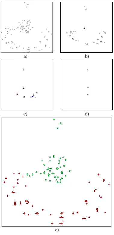
Figure 3. Illustration of the IMPACT algorithm a)-d) Moving data objects and identifying clusters e) Final result

To address this problem, we propose a clustering algorithm based on a new concept: instead of changing the centroid, we change the value of the data objects used

for clustering. By iteratively moving data objects closer together, the clusters gradually form (Fig. 3). When these movements are complete, data objects have gathered into dense regions that can be easily identified as clusters.

The main problem of clustering is the misidentification of data points at the border regions due to the effect of noise, density of the centroid and shape of the cluster. However, if we move these points closer to their centroids, which are around the crossing points of these movement vectors, the movements can increase the dissimilarities between clusters and the intracluster similarities, while the global structure of the dataset is maintained (Fig. 4).

Figure 4. Effectiveness of moving data objects

In the following sections, we introduce our clustering algorithm, which carries out clustering without specifying the number of clusters or being particularly sensitive to parameter values.

II. PROBLEM DEFINITION AND FRAMEWORK A. Problem and basic definition

Given a dataset

D



{

x

|

x



R

}

Here we introduce fundamental definitions used in this paper.

Attraction Attraction is a quantity that represents the attractive force between two data objects xi and xj:

p j i j

i ij

x

x

x

x

A

)

,

(

distance

1

)

,

(

attraction





where p (p > 0) is a user specified parameter used to adjust the effect of attraction between two data objects.

Attractive vector Attractive vector is an n-dimensional vector representing the attractive force between a data object and another data object caused by the attraction between them. Attractive vector avij = (av ij1, avij2… avijn)

of xi for xj is computed as

) .. 1 ( | |

1

n k A x x

x x

av n ij

r

ir jr

ik jk

ijk  

  





Inertia Inertia is a quantity representing the effect of a cluster on its membership. The inertia of each cluster is computed as

sterSize largestClu

C

Ij j

| |

 ,

where Cj is the j

th

cluster. |Cj| is the size of Cj and

largestClusterSize is the size of the largest cluster.

B. Framework

1) Moving data objects

Moving data objects can improve the quality of identified clusters by increasing the similarities between similar data objects and the dissimilarities between clusters. In this section, we describe how to compute the movement of a data object (movement vector).

There are three steps to compute the movement vector of a data object:

 computing the attraction,  computing the movement vector,

 computing the inertia of each cluster and the Scale value.

As in physics, objects attract each other and move closer under the effect of an attractive force among them (attraction). The effect of attraction is directly correlated to the parameter p, the quantity used to adjust the local and global distribution of datasets. If p takes a small value (e.g., 1 or 2), not only neighbors but also objects further away can affect an object. In this case, the dataset tends to reach a global balance. In contrast, if p takes a larger value (e.g., 3, 4, ...), the attraction is only toward neighbors1, and the cluster tends to maximize the intracluster similarity (see Fig. 5).

a) Moving data objects and identifying clusters using small p

b) Moving data objects and identifying clusters using large p Figure 5. Effect of parameter p on IMPACT clustering

The attractive forces shift objects, as represented by movement vector. The direction of the movement vector vi of xi is the summation of all attractive vectors of all

other data objects to xi:





 m

j ij

i av

v 1

.

The length of the movement vector should be calculated carefully. For the sake of higher clustering accuracy, the distance of movement (magnitude of the movement vector) should not be too long. However, if the distance of the movement is too short, the clustering process will be slow. In addition, after data objects form a cluster, they do not need to move so much. Based on these considerations, the movement is adjusted by two values:

 Inertia: If xi belongs to a cluster Cj, its movement

vector vi is adjusted as

) 1

( j

i

i v I

v    ,

where Ij is the inertia of cluster Cj. The inertia

avoids clusters from moving too quickly and incorrectly merging.

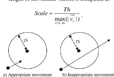
 Scale: Because the threshold value Th is used during the clustering step, the appropriate magnitude of each movement vector should be no greater than Th. Scale, a value used to adjust the length of movement vector, is computed as

| ) (| max

..

1m i

i v

Th Scale



 _.

a) Appropriate movement b) Inappropriate movement Figure 6. Appropriate and inappropriate movements of object

After adjustment, all movement vectors are guaranteed not to cross the scanning field of the nearest objects (Fig. 6). It is therefore clear that the movement of data objects retains the global and local structure of the cluster: the inertia ensures clusters do not merge easily, while computation of all the attractions affecting one data object retains the global balance.

In this step, data objects are modified (moved) as

i i

i

x

Scale

v

x







The modification increases the similarity between close objects and the dissimilarity between groups by increasing the distance of their borders. Fig. 7 summarizes the steps to move data objects.

Figure 7. Pseudocode of the moving procedure

2) Cluster identification

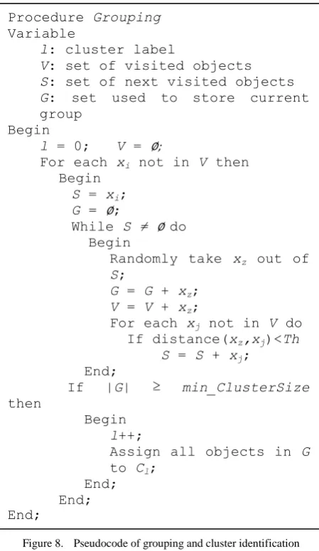
Cluster identification is the process by which indistinguishable data objects are grouped together. The pseudocode in Fig. 8 presents the steps in this process.

If the distance between two objects is less than Th, they are linked and form a group (Fig. 9). The threshold Th used in the grouping step is computed as

e maxDistanc q

Th  ,

j i j

i,x x,x

x e

maxDistanc max(distance( )) , where q is a parameter specified by the user to compute Th, the threshold value to determine whether two data objects are indistinguishable. For example, if q = 0.05, we can say that two data objects are indistinguishable if their difference is 5% less than the distance between the most different pair.

Although all data objects are assigned to groups, not all groups can be considered as clusters. A group G is a cluster if it satisfies the condition

rSize min_Cluste

G  ,

where min_ClusterSize is a threshold used to eliminate small groups.

Figure 8. Pseudocode of grouping and cluster identification

Figure 9. Illustration of grouping and cluster identification

III. IMPACT ALGORITHM

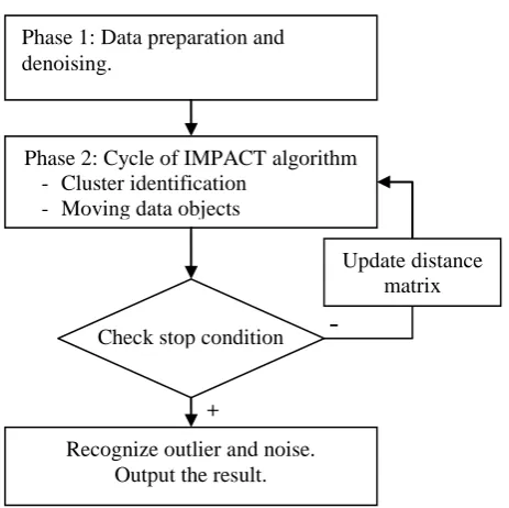
The IMPACT algorithm is based on the idea of gradually moving all objects closer to similar objects according to the attraction between them until the dataset becomes self-partitioned. The algorithm has two phases.

 Phase 1: Normalizing and denoising the input dataset.

 Phase 2: Repeating the cycle of identifying clusters and moving data objects until the stop condition is satisfied.

In this section, we describe in detail both phases as schematized in Fig. 10.

Procedure Grouping

Variable

l: cluster label

V: set of visited objects

S: set of next visited objects

G: set used to store current

group Begin

l = 0; V = ∅;

For each xi not in V then

Begin

S = xi;

G = ∅;

While S ≠ ∅ do

Begin

Randomly take xz out of

S;

G = G + xz;

V = V + xz;

For each xj not in V do

If distance(xz,xj)<Th

S = S + xj; End;

If |G| ≥ min_ClusterSize

then

Begin

l++;

Assign all objects in G

to Cl; End;

End; End;

Procedure Moving

Begin

Compute attraction matrix:

p j i j i ij

x

x

x

x

A

)

,

(

distance

1

)

,

(

attraction





Compute attractive vectors:

) .. 1 ( | | 1 n k A x x x x

av n ij

r

ir jr

ik jk

ijk  

  





avij = (av ij1, avij2… avijn)

Compute movement vector of xi:



Compute inertia for each cluster

Cj:

sterSize largestClu

C

Ij j

| | 

For each movement vector xi

If xi Cj then

Adjust xi’s movement vector

as: ) 1 ( j i i j

i C v v I

x     

Compute the Scale value:

| ) (| max

..

1m i

i v

Th Scale





Move all objects:

i i

i x Scale v

x   

End;

Figure 10. Flowchart of the IMPACT algorithm

A. Phase 1: Data preparation

The first step in this phase is to read the input data and normalize the numerical attribute values into the range [0,1]. The objective of this process is to avoid attributes with a wide range of values dominating the clustering

results. Each value in the dataset is modified as

x

x

x

x

x

rj ..m r rj ..m r

rj ..m r ij ij

)

(

min

)

(

max

)

(

min

1 1

1

 









The distance matrix is computed from this normalized dataset. The threshold Th is then computed from the maximum value of the distance matrix (i.e., longest distance).

The second step of this phase is denoising. Since we identify clusters only by grouping data objects according to the threshold Th, in noisy datasets, clusters linking at the border region can affect the recognition of clusters. However, if we simply move the data objects, noise might be reduced and the border regions become clearer, as the points move closer to their centroids and the gaps between clusters widen. The denoising step is controlled by a denoise-level parameter, which is the number of steps of moving data objects. The noisier a dataset is, the bigger this value should be. Fig.11 shows the effect of denoising.

Figure 11. Effect of denoising

B. Phase 2: Cycle of the IMPACT algorithm: cluster identification and moving data objects

The IMPACT algorithm works by iterating the grouping and moving of data objects until the dataset is self-partitioned. This section details the workings of the cycle.

Cluster identification This task has been described in the above sections. Although we choose a method based on a simple linking method in this paper, it is possible to use other clustering methods to identify the clusters (e.g., X-means and Chameleon).

Moving data objects The difference between the IMPACT algorithm and other algorithms is the movement of data objects. Most algorithms attempt clustering based on a static similarity matrix and a method to optimize a certain criterion. Our algorithm has several advantages as described below:

 Centroid determination: Owing to attraction, data objects in a border region tend to move closer to their centroid, making clusters denser and easier to detect.

 Stable results: Clustering algorithms usually produce different results for different parameters. However, because the movement of data objects in IMPACT maintains the underlying cluster structure, our method is less sensitive to parameter values.

Stop condition The iterative process stops when it meets the stop condition. The stop condition of the IMPACT algorithm can be satisfied in many ways, and not just when all data objects are clustered. Below are common stop conditions that are used for different objectives.

 A given percentage of data objects have been clustered: When all or most data objects are clustered, we can stop the cycle and deal with unclustered objects later.

 The magnitude of the longest movement vector is sufficiently small (e.g., less than Th or a user specified parameter). Data objects in dense regions are usually clustered quickly, while noisy objects and outliers are not attracted greatly by clusters.

This concept is employed by IMPACT to detect outliers and noise effectively. After detecting all clusters, outliers, and noise, the final clustering result is output. C. Example

We present a simple example to show how the IMPACT algorithm runs.

1) Dataset

The dataset has five objects as shown in Table I. In this example, the parameter set is q = 1% = 0.01 and p = 2.

2) Phase 1: Data preparation

Table II gives the dataset after normalization. The distance matrix (Table III) and threshold Th are then computed:

0.01067 067

1

1  

 

q maxDistance % .

Th .

Phase 1: Data preparation and denoising.

Phase 2: Cycle of IMPACT algorithm - Cluster identification

- Moving data objects

Check stop condition

Recognize outlier and noise. Output the result.

-

+

TABLE I. EXAMPLE DATASET

Object Attribute 1 Attribute 2

x1 3 4

x2 4 2

x3 5 7

x4 4 8

x5 2 7

TABLE II. NORMALIZED DATASET

Object Attribute 1 Attribute 2

x1 0.333 0.333

x2 0.666 0

x3 1 0.833

x4 0.666 1

x5 0 0.833

TABLE III. DISTANCE MATRIX

x1 x2 x3 x4 x5

x1 0 0.471 0.833 0.745 0.600

x2 0 0.897 1 1.067

x3 0 0.372 1

x4 0 0.687

x5 0

3) Phase2: Cycle of IMPACT

Cluster identification Using the distance matrix shown in Table III, we cluster the dataset applying the method described above. Since all distances are greater than Th, no data object is labeled.

Computing the attraction matrix As an example, we compute the attraction between x1 and x2 (A12). A12 is calculated as 5 . 4 471 . 0 1 ) , ( distance 1 ) , ( attraction ₂ 21

12   p  

j i j i x x x x A A .

Table IV presents the complete attraction matrix. TABLE IV. ATTRACTION MATRIX

x1 x2 x3 x4 x5

x1 0 4.5 1.44 1.8 2.769

x2 0 1.241 1 0.878

x3 0 7.2 1

x4 0 2.117

x5 0

Computing the attractive vector The attractive vector av12 = (av121, av122) of x1 for x2 is calculated as

ij ir jr n r ik jk ijk A x x x x av      (| | ) max 1.. , 2.25 4.5 0.666 0.333 0.666 | ) (|

max₁ 2 1 12

11 21

121  

       A x x x x av r r ..n r , 25 2 4.5 0.666 0.333 0 |) (|

max 2 1 12

1

12 22

122 A .

x x x x av r r ..n r           .

Finally, we obtain the attractive vector av12 of x1 for x2 as ) 25 2 25 2 ( = ) ( 121 122

12 = av , av . , - .

av .

TABLE V. ATTRACTIVE VECTORS AFFECTING X1

Name Aij Attractive vector (avi)

av12 4.5 (2.25, -2.25) av13 1.44 (0.822, 0.617) av14 1.8 (0.6, 1.2) av15 2.769 (-1.107, 1.661)

Table V presents the attractive forces affecting x1. After computing all attractive vectors, we compute the movement vector. The movement vector v1 of x1 is the summation of all attractive vectors, and is calculated as

1.228)

(2.565,

1







 j

j

av

v

Table VI presents the movement vectors for all data objects.

TABLE VI. MOVEMENT VECTORS

Name Movement vector v1 (2.565, 1.228) v2 (-2.285, 4.624) v3 (-6.977, 0.896) v4 (2.505, -5.023) v5 (4.192, -1.725)

We need to adjust these vectors before modifying the values of all data objects. The largest magnitude of all movement vectors is 7.034 (v3 = (-6.977, 0.896)). Scale for adjusting movement vectors is given by

001517

0

max

.

v

Scale  



.

Since there is no cluster, we can modify the movement vector without computing the inertia of each cluster:

Scale

v

v





Table VII presents the adjusted movement vector for each data object.

TABLE VII. ADJUSTED MOVEMENT VECTORS

Name Adjusted movement vector v1 (0.00389, 0.00186)

v2 (-0.00346, 0.00701)

v3 (-0.01058, 0.00135)

v4 (0.00380, -0.00762)

v5 (0.00635, -0.00261)

TABLE VIII. MODIFIED OBJECT

Object Modified object

x1 = (0.333, 0.333) (0.337, 0.335) x2 = (0.666, 0) (0.663, 0.07) x3 = (1, 0.833) (0.989, 0.835) x4 = (0.666, 1) (0.670, 0.992) x5 = (0, 0.833) (0.006, 0.830)

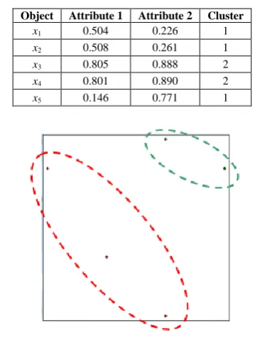
The distance matrix is updated, and the cycle described above is repeated until the stop condition is satisfied. In this example, the stop condition is satisfied when 90% of all data objects are clustered. The result is presented in Table IX and Fig. 12.

TABLE IX. FINAL MODIFIED OBJECTS AND CLUSTER LABELS

Object Attribute 1 Attribute 2 Cluster

x1 0.504 0.226 1

x2 0.508 0.261 1

x3 0.805 0.888 2

x4 0.801 0.890 2

x5 0.146 0.771 1

Figure 12. Clustering result of the IMPACT algorithm

IV. COMPLEXITY OF THE IMPACT ALGORITHM The way the IMPACT algorithm clusters the dataset is similar to the workings of affinity systems in physics, and the computational cost of this method is thus relatively high.

Some steps of our algorithm are highly complex: computing the distance matrix, attraction matrix, attractive vectors, and movement vectors. To compute the complexity of the IMPACT algorithm, we assume that the dataset has m data objects and n attributes. The computational complexity of computing the distance and attraction matrix is O(m2n). Computing an attractive vector costs n operations, so the overall complexity to compute all attractive vectors is O(m2n). Each movement vector of a data object is a summation of all attractive vectors affecting it. For each data object, there are m - 1 attractive forces affecting it, and the complexity of each operation for one additional vector is O(n). Therefore, the complexity to compute all m movement vectors is O(m2n). Hence, the overall complexity to compute these matrices is O(m2n).

Since IMPACT is an iterative algorithm, we should estimate the number of iterations. The number of iterations depends on how quickly the objects move close together (the speed of the self-partitioning process). We know that for each iteration, objects move a distance smaller than Th. Therefore, the speed of self-partitioning is directly correlated to the value of the threshold Th. The average distance between two objects is _n n_{min an}

dataset, so it will cost approximately _{n Th}n_m iterations to move an object close to another object. Since the threshold Th is usually computed as q n , the approximate number of iterations is n

m q

1 .

From the above computations, we find that the overall computational complexity of IMPACT is O( n

m q n

m2 ).

Fig. 13 shows the processing time of the IMPACT algorithm when clustering random datasets. The machine configuration used in this experiment is a T6400 Core 2 Duo central processing unit running at 2.00 GHz with 4 GB random access memory.

Figure 13. Chart of processing time

In the case of high-density datasets, the algorithm detects clusters more easily and quickly since they are well connected. In Fig. 13, the processing time for the last dataset is less. The reason is that the last dataset is denser than others, and IMPACT therefore does not need to perform many iterations to cluster it.

V. EXPERIMENTAL RESULTS

In this section, we evaluate the performance of IMPACT and demonstrate its effectiveness for different types of data distributions. We use six synthetic datasets, two datasets used in the paper presenting the Chameleon algorithm, two real datasets from the UCI Machine Learning Repository [21], and one text dataset available at [22]. We firstly introduce these eleven datasets used in this paper.

The six synthetic datasets are denoted DS1 to DS5, and DS8. DS1 and DS2 are hierarchical datasets. DS3 and DS4 contain clusters with different densities and sizes. DS5 includes many disjointed clusters (142 clusters) to demonstrate that IMPACT works well with a large number of clusters. DS6 and DS7 are datasets used to evaluate the Chameleon algorithm. DS8 is a simple hard

0 5000 10000 15000 20000 25000 30000

200 400 600 800 1000 1200 1400

Tim

e

(m

s)

Size of dataset

clustering dataset that includes 100 points generated randomly, and three 10 point clusters placed in three corners of the dataset. Wine and Iris are commonly used datasets taken from the UCI Machine Learning Repository. R8- is a sub collection of the Reuters-21578 dataset. These datasets characterize different problems in clustering. Table X gives the sizes of all datasets and the numbers of desired clusters (the correct clustering results) for them.

TABLE X. EXPERIMENT DATASETS

Dataset Size of datasets Desired number of clusters

DS1 250 2

DS2 800 3

DS3 1934 4

DS4 4343 6

DS5 8026 142

DS6 8000 6

DS7 8000 8

DS8 130 3

Iris 150 (four features) 3 Wine 178 (13 features) 3 R8- 445 documents 8

We compare clustering results obtained with IMPACT with those obtained using X-means and the Cluto toolkit. An implementation of X-means from [23], like the IMPACT algorithm, does not require a priori specification of the number of clusters. Cluto [24] is a commonly used clustering toolkit, which provides three different classes of clustering algorithms based on the partition, agglomerative, and graph partitioning paradigms. In this paper, all datasets were analyzed using the graph method implemented in Cluto (–clmethod = graph and –sim = dist). This clustering method is the motivation for Chameleon, an effective clustering algorithm.

A. Cluster identifying ability

To demonstrate the ability of the IMPACT algorithm to identify clusters, we performed clustering on DS1, DS2, DS3, DS4, and DS5, which are datasets with different cluster types.

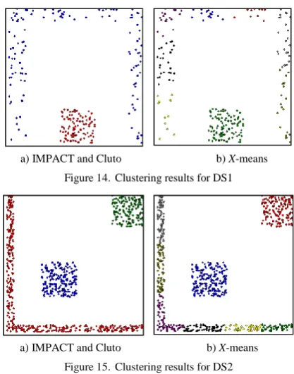
The experimental results show that partitioning clustering algorithms have difficulty handling hierarchical datasets. DS1 and DS2 contain clusters for which the centroids are not within the clusters or are located within another cluster. Figs. 14 and 15 show clustering results obtained with IMPACT, Cluto and X-means. It is clearly seen that IMPACT and Cluto outperform X-means. These results also demonstrate that IMPACT can cluster hierarchical datasets effectively.

Next, we compared our clustering results for DS3, DS4, and DS5 obtained with IMPACT with those obtained with Cluto. DS3 and DS4 (Fig. 16) are simple datasets with clusters that have different densities and sizes: the darker the cluster is, the denser it is. The clusters in these datasets have densities differing approximately five-fold and sizes differing approximately two-fold. Fig. 17 shows results obtained using IMPACT

and Cluto with default parameters. The clustering results are the same for the two clustering programs.

a) IMPACT and Cluto b) X-means Figure 14. Clustering results for DS1

a) IMPACT and Cluto b) X-means Figure 15. Clustering results for DS2

The number of clusters can affect an algorithm’s clustering result. To verify that the number of clusters does not affect IMPACT, we compared the clustering results for DS5 (Fig. 18) and found that IMPACT identified correctly all 142 clusters of DS5, while Cluto could identify 142 clusters correctly only with the parameter NNbrs set at 7 or 8. For other values of the parameter NNbrs, Cluto produced similar results1.

Figure 16. DS3 (left) and DS4 (right)

Figure 17. Clustering results for DS3 and DS4 using IMPACT and Cluto

Figure 18. DS5

Figure 19. Clustering result for DS6 and DS7 using IMPACT

Figure 20. Original dataset of DS6 and DS7

The last two datasets DS6 and DS7 were obtained from the website of the author of the Chameleon clustering algorithm [25]. These datasets are extremely difficult to cluster: they contain clusters with different shapes, noise and outliers. DS6 has a chain connecting all clusters (i.e., the single-link effect), while DS7 contains clusters with different arbitrary shapes. The gaps between clusters are small and filled with noise. The clustering results, shown in Fig. 19, are similar to the results reported in the literature [8]: most clusters are the same but in the case of DS7, IMPACT breaks the marked cluster into two smaller clusters owing to the presence of some low-density regions within (see Fig. 20).

The results demonstrate that IMPACT is quite effective in finding clusters of arbitrary shape, density, and orientation.

B. Parameter sensitivity of the IMPACT algorithm

One of the most critical clustering problems is sensitivity to input parameters. To obtain accurate clustering results, we usually need to estimate the best value of the parameters for the given dataset. The IMPACT algorithm is designed to overcome this problem.

First, we introduce a dataset used to validate the parameter sensitivity of IMPACT. DS8 has 100 points generated randomly, and three small clusters of 10 points each. DS8 does not have any “natural” clusters, so the clustering results could differ depending on the cluster validity [12]. DS8 is suitable for testing the validity of the clustering algorithm. For comparison, we ran IMPACT and X-means with default parameters (p = 2, q = 0.05, min_ClusterSize = 20%), and ran Cluto with parameter NNbrs = 3,4,5,6. Results are shown in Fig. 21.

Clustering results for DS8 obtained by running IMPACT with different parameter values of p and q are shown in Fig. 21 and Table XI. It is seen how with different values of p and q, IMPACT produces the same results with a hard clustering dataset. This result suggests that the IMPACT algorithm is not parameter sensitive.

a) IMPACT and Cluto b) X-means Figure 21. Clustering results for DS8

TABLE XI. NUMBER OF CLUSTERS IN CLUSTERING RESULTS FOR DS8

p = 1 p = 2 p = 3 q = 0.5% 3 3 3 q = 1% 3 3 3 q = 2% 3 3 3

Figure 22. Clustering results with different q and p parameter sets when set min_clusterSize = 10%

a) Three clusters b) Four clusters

c) Five clusters d) Six clusters

Figure 23. Clustering results for DS8 with min_ClusterSize = 0.1 (10%) and different sets of two parameters p and q

The experiments above suggest that the IMPACT algorithm is insensitive to changes in parameter values, and can detect clusters with different levels of specificity, which is a desirable feature for a clustering algorithm. C. Real datasets

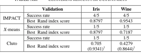
The IMPACT algorithm not only works effectively with two-dimensional datasets but also produces accurate results when dealing with real datasets. We used two common datasets from the UCI Machine Learning Repository (Wine and Iris) and one text dataset (R8-) for validation. In the case of the Wine and Iris datasets, the IMPACT algorithm found the correct number of clusters in most tests. To evaluate the accuracy of these clustering results, we used the Rand index [26] to compare results among IMPACT, Cluto and X-means. IMPACT outperformed X-means and Cluto for these datasets as seen in Table XII.

TABLE XII. CLUSTERING RESULTS FOR UCI DATASETS

Validation Iris Wine

IMPACT Success rate 4/5 4/5

Best Rand index score 0.8797 0.9543 X-means Success rate 1/5 1/5

Best Rand index score 0.8797 0.7187

Cluto

Success rate 1/5 1/5

Best Rand index score 0.705

(0.9341)1 _(0.8644)0.4279 1

The success rate in Table XII is the rate at which each algorithm identifies the number of clusters correctly in five experiments. In each experiment, the most important parameters of each algorithm are changed (p and q in the case of IMPACT, num_splits in the case of X-means, and NNbrs in the case of Cluto).

The text dataset R8- needs to be preprocessed before clustering. We used a Perl program to stem nouns and verbs to generate the dictionary and feature vector from R8-. However, because of the high dimension of feature vectors, both IMPACT and Cluto failed to identify the clusters in the dataset. To avoid this problem, we applied principal component analysis [27] to reduce the number of features. The dataset was then clustered employing IMPACT, Cluto, K-means, and an agglomerative method implemented in the Cluto toolkit (-method = agglo –crfun = i2). The results were evaluated using the Rand index and Fmeasure [28]. The results are presented in Table XIII.

TABLE XIII. CLUSTERING RESULTS FOR TEXT DATASET R8-

Algorithm Number of clusters identified

Rand

index score Fmeasure score

IMPACT 7 0.67 0.87

Cluto 1 (Fail) N/A N/A

K-means (k = 8) 8 0.72 0.92 Agglomerative

method (k = 8) 8 0.73 0.95

Even IMPACT could not detect all eight clusters, and it did not achieve the best Rand index score, but its result is remarkable because (1) IMPACT did not require the correct number of clusters and (2) the difference between the score for IMPACT and other methods is not so large. Additionally, the Fmeasure score for IMPACT is higher than other results in the literature [19] and [20].

In all the experiments described above, our algorithm was able to identify clusters accurately for most of the datasets and was insensitive to the choice of parameters.

VI. CONCLUDING REMARKS

This paper presented the IMPACT (Iteratively Moving Points based on Attraction to ClusTer data) algorithm, a novel clustering method. Employing IMPACT, each data object attracts other data objects, and the attractive forces thus draw data objects closer together. By iteratively moving objects, the dataset eventually becomes self-partitioning.

Experimental results for several datasets with a wide variety of characteristics showed that IMPACT can

determine natural clusters effectively and that it is insensitive to the choice of parameters.

In the future, we will address the verification of IMPACT for different application domains and study the effectiveness of different techniques for optimizing clustering results.

ACKNOWLEDGEMENT

This work was supported by a Grant-in-Aid for Scientific Research (c) (10215783) from Japan Society for the Promotion of Science (JSPS).

REFERENCES

[1] M. N. Murty, A. K. Jain, P. J. Flynn. “Data clustering: A

Review”, ACM Computing Surveys, Vol. 31, No. 3,

pp.264-323, 1999.

[2] J. Kleinberg. “An impossibility theorem for clustering”, in

Advances in Neural Information Processing Systems, pp.446-453, 2002.

[3] S. Mayer zu Eissen, “On Information Need and

Categorizing Search”, PhD. Dissertation, University of

Paderborn, 2007.

[4] A. K. Jain and R. C. Dubes. Algorithms for Clustering

Data, Prentice Hall, 1988.

[5] L. Kaufman, P.J. Rousseeuw. Finding Groups in Data: an

Introduction to Cluster Analysis, John Wiley & Sons, 1990.

[6] D. Pelleg, A. Moore. “X-means: Extending K-means with

Efficient Estimation of the Number of Clusters”, in

Proceedings of the Seventeenth International Conference on Machine Learning, Morgan Kaufmann, pp.727–734, 2000.

[7] S. Guha, R. Rastogi, K. Shim. “CURE: An Efficient

Clustering Algorithm for Large Databases”, in

Proceedings of the 1998 ACM SIGMOD International Conference on Management of Data, pp.73-84, 1998.

[8] G. Karypis, E. H. Han, V. Kumar. “CHAMELEON: A

Hierarchical Clustering Algorithm Using Dynamic

Modeling”, Computer, 32(8), pp.68-75, 1999.

[9] M. Ester, H. P. Kriegel, J. Sander, X. Xu. “A

Density-Based Algorithm for Discovering Clusters in Large Spatial

Databases with Noise”, in Proceedings of the 2nd

International Conference on Knowledge Discovery and Data mining, pp.226–231, 1996.

[10]M. Ankerst, M. M. Breunig, H. P. Kriegel, J. Sander.

“OPTICS: Ordering points to identify clustering structure”, in Proceedings of the ACM SIGMOD Conference, pp.49-60, 1999.

[11]A. Hinneburg, D. Keim. “An Efficient Approach to

Clustering in Large Multimedia Databases with Noise”, in

Proceeding 4th Int. Conf. on Knowledge Discovery & Data Mining, pp.58-65, 1998.

[12]A. K. Jain. “Data Clustering: 50 Years Beyond K-Means”,

Pattern Recognition Letters, 31(8), pp.651-666, 2001.

[13]W. Wang, J. Yang, R. Muntz. “STING: A Statistical

Information Grid Approach to Spatial Data Mining”, in

Proceedings of the 23rd Conference on VLDB, pp.186-195, 1997.

[14]R. Agrawal, J. Gehrke, D. Gunopulos, P. Raghavan.

“Automatic Subspace Clustering of High Dimensional

Data for Data Mining Applications”, in Proceedings of the

ACM SIGMOD Conference, pp.94-105, 1998.

[15]Y. Chen, L. Tu. “Stream Data Clustering Based on Grid

Density and Attraction”, ACM Trans. Knowl. Discov., Vol.

3, No. 3, pp.1-27, 2009.

[16]H. Azzag, N. Monmarché, M. Slimane, G. Venturini, C.

Guinot. “AntTree: a New Model for Clustering with

Artificial Ants”, in Proceeding of the CEC 2003, pp.2642–

2647. IEEE Press, 2003.

[17]M. Errecalde, D. Ingaramo, P. Rosso. “A new

AntTree-based algorithm for clustering short-text corpora”, Journal

of Computer Science and Technology, 10(1), pp.1-7, 2010.

[18]P. J. Rousseeuw. “Silhouettes: a graphical aid to the

interpretation and validation of cluster analysis”, Journal

of Computational and Applied Mathematics, Vol. 20, No. 1, pp.53-65, 1987.

[19]D. Ingaramo, M. Errecalde, P. Rosso. “A general

bio-inspired method to improve the short-text clustering task”, in Proceeding of CICLing 2010. Computational Linguistics and Intelligent Text Processing, pp.661-672, Springer, 2010.

[20]M. Errecalde, D. Ingaramo, P. Rosso. “ITSA*: An

Effective Iterative Method for Short-Text Clustering

Tasks”, in Proceedings of IEA/AIE, pp.550-559, 2010.

[21]The UCI Machine Learning Repository.

http://archive.ics.uci.edu/ml/datasets.

[22]Data Sets for Short-text Experimental Works.

https://sites.google.com/site/merrecalde/resources.

[23]K-means and KD-trees resources.

www.cs.cmu.edu/~dpelleg/kmeans.html.

[24]G. Karypis. “Cluto - A Clustering Toolkit”,

http://glaros.dtc.umn.edu/gkhome/cluto/cluto/download, 2003.

[25]Karypis Lab. Datasets.

http://glaros.dtc.umn.edu/gkhome/fetch/sw/cluto/chameleo n-data.tar.gz.

[26]L. Hubert, P. Arabie. “Comparing Partitions”. Journal of

Classification, Vol. 2, No. 1, pp.193–218, Springer, 1985.

[27]I. T. Jolliffe. Principal Component Analysis,

Springer-Verlag, 2002.

[28]J. Makhoul, F. Kubala, R. Schwartz, R. Weischedel.

“Performance measures for information extraction”, in

Proceeding of DARPA Broadcast News Workshop,

pp.249–252, 1999.

Vu Anh Tran was born in 1987, in Nha Trang, Viet Nam. He received the B.E. in Information System from Nha Trang University in 2010. He currently is a Master student of Kanazawa University. His research interests include data mining and algorithm.

Associate at the University of Colorado. He has published articles in Bioinformatics (Clemente et al. "Phylogenetic

Reconstruction from Non-Genomic Data".

Bioinformatics 23(2):e110-e115; 2007), BMC Bioinformatics (Clemente et al. "Flexible Taxonomic Assignment of Ambiguous Sequencing Reads". BMC Bioinformatics 12:8; 2011), or Science (Muegge, Kuczynski, Knights, Clemente et al "Diet Drives Convergence in Gut Microbiome Functions Across Mammalian Phylogeny and Within Humans". Science 332(6032):970-974; 2011) among others. His current research interests include analysis of metagenomic data, high-throughput genome assembly, and temporal data series analysis.

Duc Thuan Nguyen was born in Hue, Vietnam, 1962. He received his B.S. degree in Mathematics Lecturer from Hue University in 1985, M.E. degree in Information Technology from Nha Trang University in 1998, and his PhD degree from Vietnamese Academy of Science and Technology in 2011. His research interests include Rough Set, Data mining, and Distributed Database.

Jiuyong Li received his BSc degree in physics and MPhil degree in information processing from Yunnan University in China in 1987 and 1998 respectively, and received his PhD degree in computer science from Griffith University in Australia in 2002. He is currently an associate professor at University of South Australia. His main research interests are in data mining, privacy preservation and bioinformatics. His research has been supported by Australian Research Council Discovery grants multiple times. He has more than fifty journal and conference publications. He has chaired Australasian Data Mining Conference and Australasian Joint Conference on Artificial Intelligence.

Xuan ThoDang was born in 1985, in Vietnam. He received the B.S., M.S. degrees in computer science from Hanoi National University of Education, in 2007, 2009 respectively.

He was a lecturer of Hanoi National

University of Education, Hanoi,

Vietnam (2007-2010). From 2010 to

2011, he was a PhD student of Kanazawa University, Ishikawa, Japan. He is currently a PhD student of Kanazawa University, Ishikawa, Japan. His research interests include bioinformatics.

Thi Tu Kien Le received the B.S. degrees in computer science from Hanoi University of Education, Vietnam in 1999. She received the M.S. degrees in computer science from Hanoi University of Science and Technology, Vietnam in 2003.

She is a lecturer in Faculty of

Information Technology of Hanoi

University of Education, Vietnam. He is currently a PhD student of Kanazawa University, Ishikawa, Japan. Her research interests include the topics in bioinformatics.

Thi Lan Anh Nguyen was born in 1984, in Hue, Vietnam. She received the B.S. and M.E. degrees in computer science from Hue University- Vietnam, in 2006 and 2008, respectively.

She is currently a Doctoral student of Kanazawa University, Ishikawa, Japan. Her research topics interests include the topics in bioinformatics.

Thammakorn Saethang was born in 1985, in Chiang Mai, Thailand. He

received the B.E. degrees in

Biotechnology from Chiang Mai

University and M.E. degrees in

Bioinformatics from King Mongkut's University of Technology Thonburi, in 2007 and 2009, respectively.

He is currently a PhD student of Kanazawa University, Ishikawa, Japan. His research topics interests include immunoinformatics and bioinformatics.

Mamoru Kubo received B.E. and M.E. degrees from Nagoya Institute of

Technology in 1990 and 1992,

respectively. He is an assistant professor in Faculty of Electrical and Computer Engineering at Kanazawa University, Japan. His research interests include

pattern recognition and image

processing. He is a member of IEEE.

Yoichi Yamada received B.S. degree from Tsukuba University in 1996. He received M.S. and D.M. degrees in biological science and medical science from Tokyo University in 1998 and 2002, respectively. He is a Lecturer in the Faculty of Electrical and Computer Engineering, Institute of Science and Engineering at Kanazawa University, Japan. His research

interests include molecular biology and bioinformatics.

Kenji Satou was born in 1963, in Fukuoka, Japan. He received the B.E., M.E., and D.E. degrees in computer science and communication engineering from Kyushu University, in 1987, 1989, and 1996, respectively.