Proceedings of the 2019 Conference on Empirical Methods in Natural Language Processing 5185
TuckER: Tensor Factorization for Knowledge Graph Completion
Ivana Balaˇzevi´c1 Carl Allen1 Timothy M. Hospedales1,2
1School of Informatics, University of Edinburgh, UK
2 Samsung AI Centre, Cambridge, UK
{ivana.balazevic, carl.allen, t.hospedales}@ed.ac.uk
Abstract
Knowledge graphs are structured representa-tions of real world facts. However, they typ-ically contain only a small subset of all pos-sible facts. Link prediction is a task of infer-ring missing facts based on existing ones. We propose TuckER, a relatively straightforward but powerful linear model based on Tucker decomposition of the binary tensor represen-tation of knowledge graph triples. TuckER outperforms previous state-of-the-art models across standard link prediction datasets, act-ing as a strong baseline for more elaborate models. We show that TuckER is a fully ex-pressive model, derive sufficient bounds on its embedding dimensionalities and demonstrate that several previously introduced linear mod-els can be viewed as special cases of TuckER.
1 Introduction
Vast amounts of information available in the world can be represented succinctly asentitiesand rela-tionsbetween them. Knowledge graphsare large, graph-structured databases which store facts in triple form(es, r, eo), withesandeo representing subject and object entities andra relation. How-ever, far from all available information is currently stored in existing knowledge graphs and manually adding new information is costly, which creates the need for algorithms that are able to automat-ically infer missing facts.
Knowledge graphs can be represented as a third-order binary tensor, where each element cor-responds to a triple, 1 indicating a true fact and 0 indicating the unknown (either a false or a miss-ing fact). The task oflink predictionis to predict whether two entities are related, based on known facts already present in a knowledge graph, i.e. to infer which of the 0 entries in the tensor are indeed false, and which are missing but actually true.
A large number of approaches to link prediction so far have been linear, based on various meth-ods of factorizing the third-order binary tensor
(Nickel et al., 2011; Yang et al., 2015;Trouillon
et al.,2016;Kazemi and Poole, 2018). Recently,
state-of-the-art results have been achieved using non-linear convolutional models (Dettmers et al.,
2018;Balaˇzevi´c et al., 2019). Despite achieving
very good performance, the fundamental problem with deep, linear models is that they are non-transparent and poorly understood, as opposed to more mathematically principled and widely stud-ied tensor decomposition models.
In this paper, we introduce TuckER (E stands for entities, R for relations), a straightforward linear model for link prediction on knowledge graphs, based on Tucker decomposition (Tucker, 1966) of the binary tensor of triples, acting as a strong baseline for more elaborate models. Tucker decomposition, used widely in machine learning
(Schein et al.,2016;Ben-Younes et al.,2017;Yang
and Hospedales, 2017), factorizes a tensor into
a core tensor multiplied by a matrix along each mode. It can be thought of as a form of higher-order SVD in the special case where matrices are orthogonal and the core tensor is “all-orthogonal”
(Kroonenberg and De Leeuw,1980). In our case,
rows of the matrices contain entity and relation embeddings, while entries of the core tensor deter-mine the level of interaction between them. Sub-ject and obSub-ject entity embedding matrices are as-sumed equivalent, i.e. we make no distinction be-tween the embeddings of an entity depending on whether it appears as a subject or as an object in a particular triple. Due to the low rank of the core tensor, TuckER benefits frommulti-task learning by parameter sharing across relations.
that TuckER is fully expressive, i.e. given any ground truth over the triples, there exists an as-signment of values to the entity and relation em-beddings that accurately separates the true triples from false ones. We also derive a dimensionality bound which guarantees full expressiveness.
Finally, we show that several previous state-of-the-art linear models, RESCAL (Nickel et al., 2011), DistMult (Yang et al., 2015), ComplEx
(Trouillon et al., 2016) and SimplE (Kazemi and
Poole,2018), are special cases of TuckER.
In summary, key contributions of this paper are:
• proposing TuckER, a new linear model for link prediction on knowledge graphs, that is simple, expressive and achieves state-of-the-art resultsacross all standard datasets; • proving that TuckER is fully expressive and
deriving a bound on the embedding dimen-sionality for full expressiveness; and
• showing how TuckER subsumes several pre-viously proposed tensor factorization ap-proaches to link prediction.
2 Related Work
Severallinearmodels for link prediction have pre-viously been proposed:
RESCAL (Nickel et al.,2011) optimizes a scor-ing function containscor-ing a bilinear product between subject and object entity vectors and a full rank relation matrix. Although a very expressive and powerful model, RESCAL is prone to overfitting due to its large number of parameters, which in-creases quadratically in the embedding dimension with the number of relations in a knowledge graph. DistMult (Yang et al., 2015) is a special case of RESCAL with a diagonal matrix per relation, which reduces overfitting. However, the linear transformation performed on entity embedding vectors in DistMult is limited to a stretch. The binary tensor learned by DistMult is symmetric in the subject and object entity mode and thus Dist-Mult cannot model asymmetric relations.
ComplEx (Trouillon et al., 2016) extends Dist-Mult to the complex domain. Subject and object entity embeddings for the same entity are complex conjugates, which introduces asymmetry into the tensor decomposition and thus enables ComplEx to model asymmetric relations.
SimplE (Kazemi and Poole, 2018) is based on Canonical Polyadic (CP) decomposition ( Hitch-cock, 1927), in which subject and object entity
embeddings for the same entity are independent (note that DistMult is a special case of CP). Sim-plE’s scoring function alters CP to make subject and object entity embedding vectors dependent on each other by computing the average of two terms, first of which is a bilinear product of the subject entity head embedding, relation embedding and object entity tail embedding and the second is a bilinear product of the object entity head embed-ding, inverse relation embedding and subject en-tity tail embedding.
Recently, state-of-the-art results have been achieved withnon-linearmodels:
ConvE(Dettmers et al.,2018) performs a global 2D convolution operation on the subject entity and relation embedding vectors, after they are re-shaped to matrices and concatenated. The ob-tained feature maps are flattened, transformed through a linear layer, and the inner product is taken with all object entity vectors to generate a score for each triple. Whilst results achieved by ConvE are impressive, its reshaping and concate-nating of vectors as well as using 2D convolution on word embeddings is unintuitive.
HypER (Balaˇzevi´c et al., 2019) is a simplified convolutional model, that uses a hypernetwork to generate 1D convolutional filters for each relation, extracting relation-specific features from subject entity embeddings. The authors show that convo-lution is a way of introducing sparsity and param-eter tying and that HypER can be understood in terms of tensor factorization up to a non-linearity, thus placing HypER closer to the well established family of factorization models. The drawback of HypER is that it sets most elements of the core weight tensor to 0, which amounts to hard regular-ization, rather than letting the model learn which parameters to use via soft regularization.
Scoring functions of all models described above and TuckER are summarized in Table1.
3 Background
LetEdenote the set of all entities andRthe set of all relations present in a knowledge graph. A triple is represented as (es, r, eo), with es, eo ∈ E de-noting subject and object entities respectively and
r∈ Rthe relation between them.
3.1 Link Prediction
Model Scoring Function Relation Parameters Space Complexity
RESCAL (Nickel et al.,2011) e>sWreo Wr∈Rde
2
O(nede+nrd2r) DistMult (Yang et al.,2015) hes,wr,eoi wr∈Rde O(n
ede+nrde) ComplEx (Trouillon et al.,2016) Re(hes,wr,eoi) wr∈Cde O(n
ede+nrde) ConvE (Dettmers et al.,2018) f(vec(f([es;wr]∗w))W)eo wr∈Rdr O(nede+nrdr) SimplE (Kazemi and Poole,2018) 12(hhes,wr,teoi+hheo,wr−1,tesi) wr∈R
de O(n
ede+nrde) HypER (Balaˇzevi´c et al.,2019) f(vec(es∗vec−1(wrH))W)eo wr∈Rdr O(n
ede+nrdr)
TuckER (ours) W ×1es×2wr×3eo wr∈Rdr O(n
ede+nrdr)
Table 1: Scoring functions of state-of-the-art link prediction models, the dimensionality of their relation param-eters, and significant terms of their space complexity. de anddr are the dimensionalities of entity and relation
embeddings, whileneandnrdenote the number of entities and relations respectively. eo ∈Cde is the complex
conjugate ofeo,es,wr ∈R
dw×dh denote a 2D reshaping ofe
sandwrrespectively,hes,tes ∈R
de are the head
and tail entity embedding of entityes, andwr−1 ∈Rdr is the embedding of relationr−1(which is the inverse of
relationr).∗is the convolution operator,h·idenotes the dot product and×ndenotes the tensor product along the n-th mode,f is a non-linear function, andW ∈Rde×de×dr is the core tensor of a Tucker decomposition.
that assigns a scores = φ(es, r, eo) ∈ Rwhich indicates whether a triple is true, with the ultimate goal of being able to correctly score all missing triples. The scoring function is either a specific form of tensor factorization in the case of linear models or a more complex (deep) neural network architecture for non-linear models. Typically, a positive score for a particular triple indicates a true fact predicted by the model, while a negative score indicates a false one. With most recent models, a non-linearity such as the logistic sigmoid function is typically applied to the score to give a corre-sponding probability predictionp=σ(s) ∈[0,1] as to whether a certain fact is true.
3.2 Tucker Decomposition
Tucker decomposition, named after Ledyard R. Tucker (Tucker,1964), decomposes a tensor into a set of matrices and a smaller core tensor. In a three-mode case, given the original tensor X ∈ RI×J×K, Tucker decomposition outputs a tensor Z ∈ RP×Q×R and three matrices A ∈
RI×P, B∈RJ×Q,C∈
RK×R:
X ≈ Z ×1A×2B×3C, (1)
with×nindicating the tensor product along the n-th mode. Factor matricesA, BandC, when or-thogonal, can be thought of as the principal com-ponents in each mode. Elements of thecore tensor Zshow the level of interaction between the differ-ent compondiffer-ents. Typically, P, Q, R are smaller thanI,J,K respectively, soZ can be thought of as a compressed version ofX. Tucker decomposi-tion is not unique, i.e. we can transformZwithout affecting the fit if we apply the inverse transforma-tion toA,BandC(Kolda and Bader,2009).
4 Tucker Decomposition for Link
Prediction
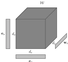
We propose a model that uses Tucker decomposi-tion for link predicdecomposi-tion on the binary tensor rep-resentation of a knowledge graph, with entity em-bedding matrixEthat is equivalent for subject and object entities, i.e. E = A = C ∈ Rne×de and relation embedding matrix R = B ∈ Rnr×dr, whereneandnr represent the number of entities and relations anddeanddr the dimensionality of entity and relation embedding vectors.
W
de de
dr es
eo
[image:3.595.346.481.431.554.2]wr
Figure 1: Visualization of the TuckER architecture.
We define the scoring function for TuckER as:
φ(es, r, eo) =W ×1es×2wr×3eo, (2)
wherees,eo∈Rdeare the rows ofErepresenting the subject and object entity embedding vectors,
wr∈Rdr the rows ofRrepresenting the relation embedding vector andW ∈Rde×dr×deis the core tensor. We apply logistic sigmoid to each score
respect to entity and relation embedding dimen-sionalitydeanddr, as the number of entities and relations increases, since the number of parame-ters ofW depends only on the entity and relation embedding dimensionality and not on the number of entities or relations. By having the core tensor W, unlike simpler models such as DistMult, Com-plEx and SimplE, TuckER does not encode all the learned knowledge into the embeddings; some is stored in the core tensor and shared between all entities and relations throughmulti-task learning. Rather than learning distinct relation-specific ma-trices, the core tensor of TuckER can be viewed as containing a shared pool of “prototype” relation matrices, which are linearly combined according to the parameters in each relation embedding.
4.1 Training
Since the logistic sigmoid is applied to the scor-ing function to approximate the true binary ten-sor, the implicit underlying tensor is comprised of −∞and∞. Given this prevents an explicit ana-lytical factorization, we use numerical methods to train TuckER. We use the standard data augmenta-tion technique, first used byDettmers et al.(2018) and formally described by Lacroix et al. (2018), of adding reciprocal relations for every triple in the dataset, i.e. we add (eo, r−1, es) for every (es, r, eo). Following the training procedure intro-duced byDettmers et al.(2018) to speed up train-ing, we use 1-N scoring, i.e. we simultaneously score entity-relation pairs (es, r) and (eo, r−1) with all entities eo ∈ E and es ∈ E respec-tively, in contrast to1-1 scoring, where individual triples(es, r, eo) and(eo, r−1, es)are trained one at a time. The model is trained to minimize the Bernoulli negative log-likelihood loss function. A component of the loss for one entity-relation pair with all others entities is defined as:
L=− 1
ne
ne
P
i=1
(y(i)log(p(i)) + (1−y(i))log(1−p(i))),
(3) wherep ∈ Rne is the vector of predicted proba-bilities andy∈Rne is the binary label vector.
5 Theoretical Analysis
5.1 Full Expressiveness and Embedding Dimensionality
A tensor factorization model is fully expressive if for any ground truth over all entities and rela-tions, there exist entity and relation embeddings
that accurately separate true triples from the false. As shown in (Trouillon et al.,2017), ComplEx is fully expressive with the embedding dimensional-ity boundde = dr = ne·nr. Similarly to Com-plEx,Kazemi and Poole(2018) show that SimplE is fully expressive with entity and relation embed-dings of sizede=dr=min(ne·nr, γ+ 1), where
γ represents the number of true facts. They fur-ther prove ofur-ther models are not fully expressive: DistMult, because it cannot model asymmetric re-lations; and transitive models such as TransE (
Bor-des et al., 2013) and its variants FTransE (Feng
et al., 2016) and STransE (Nguyen et al., 2016),
because of certain contradictions that they impose between different relation types. By Theorem1, we establish the bound on entity and relation em-bedding dimensionality (i.e. decomposition rank) that guarantees full expressiveness of TuckER.
Theorem 1. Given any ground truth over a set of entitiesE and relationsR, there exists a TuckER model with entity embeddings of dimensionality
de = ne and relation embeddings of
dimension-ality dr = nr, where ne = |E| is the number of
entities andnr =|R|the number of relations, that
accurately represents that ground truth.
Proof. Letes andeo be thene-dimensional one-hot binary vector representations of subject and object entities es and eo respectively andwr the
nr-dimensional one-hot binary vector representa-tion of relarepresenta-tionr. For each subject entitye(si), rela-tionr(j)and object entitye(ok), we let thei-th,j-th andk-th element respectively of the corresponding vectorses,wr andeo be 1 and all other elements 0. Further, we set the ijk element of the tensor W ∈ Rne×nr×ne to 1 if the fact (e
s, r, eo) holds and -1 otherwise. Thus the product of the entity embeddings and the relation embedding with the core tensor, after applying the logistic sigmoid, ac-curately represents the original tensor.
bilin-11 11
11 11
11 11
(a) DistMult
11 11
111 11
11 1
11 11
11
−1−1 −1−1
−1−1
(b) ComplEx
1 2 1 2 1 2 1 2 1 2 1 2
1 2 1 2 1 2 1 2 1 2 1 2
[image:5.595.161.437.61.161.2](c) SimplE
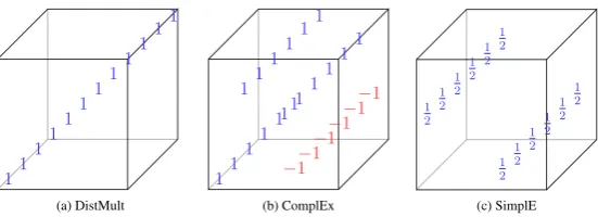
Figure 2: Constraints imposed on the values of core tensorZ ∈Rde×de×defor DistMult andZ ∈
R2de×2de×2de
for ComplEx and SimplE. Elements that are set to 0 are represented in white.
ear link prediction model, forcing it to learn that structure and generalize to new data, rather than simply memorizing the input. In general, we ex-pect TuckER to perform better than ComplEx and SimplE with embeddings of lower dimensionality due to parameter sharing in the core tensor (shown empirically in Section6.4), which could be of im-portance for efficiency in downstream tasks.
5.2 Relation to Previous Linear Models
Several previous tensor factorization models can be viewed as a special case of TuckER:
RESCAL (Nickel et al., 2011) Following the notation introduced in Section3.2, the RESCAL scoring function (see Table1) has the form:
X ≈ Z ×1A×3C. (4)
This corresponds to Equation1withI =K =ne,
P =R=de,Q=J =nrandB=IJ theJ×J identity matrix. This is also known as Tucker2 de-composition (Kolda and Bader, 2009). As is the case with TuckER, the entity embedding matrix of RESCAL is shared between subject and object en-tities, i.e. E = A = C ∈ Rne×de and the rela-tion matricesWr∈Rde×de are thede×deslices of the core tensorZ. As mentioned in Section2, the drawback of RESCAL compared to TuckER is that its number of parameters growsquadratically in the entity embedding dimensiondeas the num-ber of relations increases.
DistMult (Yang et al.,2015) The scoring func-tion of DistMult (see Table 1) can be viewed as equivalent to that of TuckER (see Equation1) with a core tensorZ ∈ RP×Q×R,P = Q =R =d
e, which issuperdiagonalwith 1s on the superdiag-onal, i.e. all elementszpqr with p = q = r are 1 and all the other elements are 0 (as shown in Figure 2a). Rows of E = A = C ∈ Rne×de contain subject and object entity embedding vec-torses,eo ∈ Rde and rows ofR =B ∈Rnr×de contain relation embedding vectorswr ∈ Rde. It
is interesting to note that the TuckER interpreta-tion of the DistMult scoring funcinterpreta-tion, given that matricesA andCare identical, can alternatively be interpreted as a special case of CP decomposi-tion (Hitchcock, 1927), since Tucker decomposi-tion with a superdiagonal core tensor is equivalent to CP decomposition. Due to enforced symmetry in subject and object entity mode, DistMult cannot learn to represent asymmetric relations.
ComplEx (Trouillon et al., 2016) Bilinear modelsrepresent subject and object entity embed-dings as vectorses,eo ∈Rde, relation as a matrix Wr ∈ Rde×de and the scoring function as a bi-linear productφ(es, r, eo) = esWreo. It is trivial to show that both RESCAL and DistMult belong to the family of bilinear models. As explained by
Kazemi and Poole(2018), ComplEx can be
con-sidered a bilinear model with the real and imagi-nary part of an embedding for each entity concate-nated in a single vector,[Re(es);Im(es)] ∈ R2de for subject, [Re(eo);Im(eo)] ∈ R2de for object, and a relation matrixWr∈R2de×2de, constrained so that its leading diagonal contains duplicated elements of Re(wr), its de-diagonal elements of Im(wr)and its -de-diagonal elements of -Im(wr), with all other elements set to 0, wheredeand -de represent offsets from the leading diagonal.
Similarly to DistMult, we can regard the scoring function of ComplEx (see Table1) as equivalent to the scoring function of TuckER (see Equation 1), with core tensor Z ∈ RP×Q×R, P = Q =
SimplE (Kazemi and Poole,2018) The authors show that SimplE belongs to the family of bilinear models by concatenating embeddings for head and tail entities for both subject and object into vec-tors[hes;tes] ∈ R
2de and[h
eo;teo] ∈ R
2de and
constraining the relation matrix Wr ∈ R2de×2de so that it contains the relation embedding vector
1
2wr on its de-diagonal and the inverse relation
embedding vector 12wr−1 on its -de-diagonal and 0s elsewhere. The SimplE scoring function (see Table1) is therefore equivalent to that of TuckER (see Equation1), with core tensorZ ∈ RP×Q×R,
P = Q =R = 2de, where2de elements on two tensor diagonals are set to12 and all other elements are set to 0 (see Figure2c).
5.3 Representing Asymmetric Relations
Each relation in a knowledge graph can be charac-terized by a certain set of properties, such as sym-metry, reflexivity, transitivity. So far, there have been two possible ways in which linear link pre-diction models introduce asymmetry into factor-ization of the binary tensor of triples:
• distinct (although possibly related) embed-dings for subject and object entities and a di-agonal matrix (or equivalently a vector) for each relation, as is the case with models such as ComplEx and SimplE; or
• equivalent subject and object entity embed-dings and each relation represented by a full rank matrix, which is the case with RESCAL.
The latter approach appears more intuitive, since asymmetry is a property of the relation, rather than the entities. However, the drawback of the latter approach is quadratic growth of parameter number with the number of relations, which of-ten leads to overfitting, especially for relations with a small number of training triples. TuckER overcomes this by representing relations as vec-torswr, which makes the parameter number grow linearly with the number of relations, while still keeping the desirable property of allowing rela-tions to be asymmetric by having an asymmetric relation-agnostic core tensor W, rather than coding the relation-specific information in the en-tity embeddings. Multiplying W ∈ Rde×dr×de withwr ∈Rdr along the second mode, we obtain a full rank relation-specific matrixWr ∈Rde×de, which can perform all possible linear transforma-tions on the entity embeddings, i.e. rotation, re-flection or stretch, and is thus also capable of
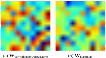
modeling asymmetry. Regardless of what kind of transformation is needed for modeling a particu-lar relation, TuckER can learn it from the data. To demonstrate this, we show sample heatmaps of learned relation matricesWrfor a WordNet sym-metric relation “derivationally related form” and an asymmetric relation “hypernym” in Figure 3, where one can see that TuckER learns to model the symmetric relation with the relation matrix that is approximately symmetric about the main diago-nal, whereas the matrix belonging to the asymmet-ric relation exhibits no obvious structure.
(a)Wderivationally related form (b)Whypernym
Figure 3: Learned relation matrices for a symmetric (derivationally related form) and an asymmetric (hy-pernym) WN18RR relation. Wderivationally related form is
approximately symmetric about the leading diagonal.
6 Experiments and Results
6.1 Datasets
We evaluate TuckER using four standard link pre-diction datasets (see Table2):
FB15k (Bordes et al., 2013) is a subset of Free-base, a large database of real world facts.
FB15k-237 (Toutanova et al., 2015) was created from FB15k by removing the inverse of many re-lations that are present in the training set from val-idation and test sets, making it more difficult for simple models to do well.
WN18(Bordes et al.,2013) is a subset of
Word-Net, a hierarchical database containing lexical re-lations between words.
WN18RR (Dettmers et al., 2018) is a subset of WN18, created by removing the inverse relations from validation and test sets.
6.2 Implementation and Experiments
We implement TuckER in PyTorch (Paszke et al., 2017) and make our code available on GitHub.1
We choose all hyper-parameters by random search based on validation set performance. For
[image:6.595.313.520.233.347.2]FB15k and FB15k-237, we set entity and relation embedding dimensionality tode=dr= 200. For WN18 and WN18RR, which both contain a sig-nificantly smaller number of relations relative to the number of entities as well as a small num-ber of relations compared to FB15k and FB15k-237, we set de = 200 and dr = 30. We use batch normalization (Ioffe and Szegedy,2015) and dropout (Srivastava et al.,2014) to speed up train-ing. We find that lower dropout values (0.1,0.2) are required for datasets with a higher number of training triples per relation and thus less risk of overfitting (WN18 and WN18RR), whereas higher dropout values(0.3,0.4,0.5)are required for FB15k and FB15k-237. We choose the learn-ing rate from {0.01,0.005,0.003,0.001,0.0005} and learning rate decay from{1,0.995,0.99}. We find the following combinations of learning rate and learning rate decay to give the best results: (0.003,0.99)for FB15k,(0.0005,1.0)for FB15k-237,(0.005,0.995)for WN18 and(0.01,1.0)for WN18RR (see Table 5 in the Appendix A for a complete list of hyper-parameter values on each dataset). We train the model using Adam (Kingma
and Ba,2015) with the batch size 128.
At evaluation time, for each test triple we gen-erate ne candidate triples by combining the test entity-relation pair with all possible entities E, ranking the scores obtained. We use the filtered setting (Bordes et al., 2013), i.e. all known true triples are removed from the candidate set ex-cept for the current test triple. We use evaluation metrics standard across the link prediction liter-ature: mean reciprocal rank (MRR) and hits@k,
k ∈ {1,3,10}. Mean reciprocal rank is the aver-age of the inverse of the mean rank assigned to the true triple over all candidate triples. Hits@k mea-sures the percentage of times a true triple is ranked within the topkcandidate triples.
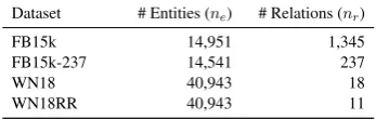
Dataset # Entities (ne) # Relations (nr)
FB15k 14,951 1,345
FB15k-237 14,541 237
WN18 40,943 18
[image:7.595.94.268.603.658.2]WN18RR 40,943 11
Table 2: Dataset statistics.
6.3 Link Prediction Results
Link prediction results on all datasets are shown in Tables3and4. Overall, TuckER outperforms pre-vious state-of-the-art models on all metrics across all datasets (apart from hits@10 on WN18 where
a non-linear model, R-GCN, does better). Re-sults achieved by TuckER are not only better than those of other linear models, such as DistMult, ComplEx and SimplE, but also better than the re-sults of many more complex deep neural network and reinforcement learning architectures, e.g. R-GCN, MINERVA, ConvE and HypER, demon-strating the expressive power of linear models and supporting our claim that simple linear models should serve as a baseline before moving onto more elaborate models.
Even with fewer parameters than ComplEx and SimplE at de = 200 and dr = 30 on WN18RR (∼9.4 vs∼16.4 million), TuckER consistently ob-tains better results than any of those models. We believe this is because TuckER exploits knowl-edge sharing between relations through the core tensor, i.e. multi-task learning. This is supported by the fact that the margin by which TuckER out-performs other linear models is notably increased on datasets with a large number of relations. For example, improvement on FB15k is +14% over ComplEx and +8% over SimplE on the tough-est hits@1 metric. To our knowledge,
ComplEx-N3 (Lacroix et al., 2018) is the only other
lin-ear link prediction model that benefits from multi-task learning. There, rank regularization of the embedding matrices is used to encourage a low-rank factorization, thus forcing parameter sharing between relations. We do not include their pub-lished results in Tables3and4, since they use the highly non-standard de = dr = 2000 and thus a far larger parameter number (18x more parameters than TuckER on WN18RR; 5.5x on FB15k-237), making their results incomparable to those typi-cally reported, including our own. However, run-ning their model with equivalent parameter num-ber to TuckER shows comparable performance, supporting our belief that the two models both at-tain the benefits of multi-task learning, although by different means.
6.4 Influence of Parameter Sharing
WN18RR FB15k-237
Linear MRR Hits@10 Hits@3 Hits@1 MRR Hits@10 Hits@3 Hits@1
DistMult (Yang et al.,2015) yes .430 .490 .440 .390 .241 .419 .263 .155
ComplEx (Trouillon et al.,2016) yes .440 .510 .460 .410 .247 .428 .275 .158
Neural LP (Yang et al.,2017) no − − − − .250 .408 − −
R-GCN (Schlichtkrull et al.,2018) no − − − − .248 .417 .264 .151
MINERVA (Das et al.,2018) no − − − − − .456 − −
ConvE (Dettmers et al.,2018) no .430 .520 .440 .400 .325 .501 .356 .237
HypER (Balaˇzevi´c et al.,2019) no .465 .522 .477 .436 .341 .520 .376 .252
M-Walk (Shen et al.,2018) no .437 − .445 .414 − − − −
RotatE (Sun et al.,2019) no − − − − .297 .480 .328 .205
[image:8.595.116.485.60.181.2]TuckER (ours) yes .470 .526 .482 .443 .358 .544 .394 .266
Table 3: Link prediction results on WN18RR and FB15k-237. The RotatE (Sun et al.,2019) results are reported without their self-adversarial negative sampling (see Appendix H in the original paper) for fair comparison.
WN18 FB15k
Linear MRR Hits@10 Hits@3 Hits@1 MRR Hits@10 Hits@3 Hits@1
TransE (Bordes et al.,2013) no − .892 − − − .471 − −
DistMult (Yang et al.,2015) yes .822 .936 .914 .728 .654 .824 .733 .546
ComplEx (Trouillon et al.,2016) yes .941 .947 .936 .936 .692 .840 .759 .599
ANALOGY (Liu et al.,2017) yes .942 .947 .944 .939 .725 .854 .785 .646
Neural LP (Yang et al.,2017) no .940 .945 − − .760 .837 − −
R-GCN (Schlichtkrull et al.,2018) no .819 .964 .929 .697 .696 .842 .760 .601
TorusE (Ebisu and Ichise,2018) no .947 .954 .950 .943 .733 .832 .771 .674
ConvE (Dettmers et al.,2018) no .943 .956 .946 .935 .657 .831 .723 .558
HypER (Balaˇzevi´c et al.,2019) no .951 958 .955 .947 .790 .885 .829 .734
SimplE (Kazemi and Poole,2018) yes .942 .947 .944 .939 .727 .838 .773 .660
[image:8.595.116.483.226.354.2]TuckER (ours) yes .953 .958 .955 .949 .795 .892 .833 .741
Table 4: Link prediction results on WN18 and FB15k.
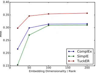
(see Table 6 in the Appendix Afor exact hyper-parameter values used) and train all three models on FB15k-237 with embedding sizes de = dr ∈ {20,50,100,200}. Figure 4 shows the obtained MRR on the test set for each model. It is important to note that at embedding dimensionalities 20, 50 and 100, TuckER has fewer parameters than Com-plEx and SimplE (e.g. ComCom-plEx and SimplE have ∼3 million and TuckER has∼2.5 million param-eters for embedding dimensionality 100).
0 50 100 150 200
Embedding Dimensionality / Rank 0.15
0.20 0.25 0.30 0.35 0.40
MRR
ComplEx SimplE TuckER
Figure 4: MRR for ComplEx, SimplE and TuckER for different embeddings sizes on FB15k-237.
We can see that the difference between the MRRs of ComplEx, SimplE and TuckER is ap-proximately constant for embedding sizes 100 and 200. However, for lower embedding sizes, the
dif-ference between MRRs increases by0.7%for em-bedding size 50 and by4.2%for embedding size 20 for ComplEx and by 3% for embedding size 50 and by 9.9% for embedding size 20 for Sim-plE. At embedding size 20 (∼300k parameters), the performance of TuckER is almost as good as the performance of ComplEx and SimplE at em-bedding size 200 (∼6 million parameters), which supports our initial assumption.
7 Conclusion
[image:8.595.101.259.544.665.2]Acknowledgements
Ivana Balaˇzevi´c and Carl Allen were supported by the Centre for Doctoral Training in Data Science, funded by EPSRC (grant EP/L016427/1) and the University of Edinburgh.
References
Ivana Balaˇzevi´c, Carl Allen, and Timothy M Hospedales. 2019. Hypernetwork Knowledge Graph Embeddings. InInternational Conference on Artificial Neural Networks.
Hedi Ben-Younes, R´emi Cadene, Matthieu Cord, and Nicolas Thome. 2017. MUTAN: Multimodal Tucker Fusion for Visual Question Answering. In
International Conference on Computer Vision.
Antoine Bordes, Nicolas Usunier, Alberto Garcia-Duran, Jason Weston, and Oksana Yakhnenko. 2013. Translating Embeddings for Modeling Multi-relational Data. InAdvances in Neural Information Processing Systems.
Rajarshi Das, Shehzaad Dhuliawala, Manzil Zaheer, Luke Vilnis, Ishan Durugkar, Akshay Krishna-murthy, Alex Smola, and Andrew McCallum. 2018. Go for a Walk and Arrive at the Answer: Reason-ing over Paths in Knowledge Bases UsReason-ing Rein-forcement Learning. InInternational Conference on Learning Representations.
Tim Dettmers, Pasquale Minervini, Pontus Stenetorp, and Sebastian Riedel. 2018. Convolutional 2D Knowledge Graph Embeddings. InAssociation for the Advancement of Artificial Intelligence.
Takuma Ebisu and Ryutaro Ichise. 2018. TorusE: Knowledge Graph Embedding on a Lie Group. In
Association for the Advancement of Artificial Intel-ligence.
Jun Feng, Minlie Huang, Mingdong Wang, Mantong Zhou, Yu Hao, and Xiaoyan Zhu. 2016. Knowledge Graph Embedding by Flexible Translation. In Prin-ciples of Knowledge Representation and Reasoning.
Frank L Hitchcock. 1927. The Expression of a Ten-sor or a Polyadic as a Sum of Products. Journal of Mathematics and Physics, 6(1-4):164–189.
Sergey Ioffe and Christian Szegedy. 2015. Batch Nor-malization: Accelerating Deep Network Training by Reducing Internal Covariate Shift. InInternational Conference on Machine Learning.
Seyed Mehran Kazemi and David Poole. 2018. Sim-plE Embedding for Link Prediction in Knowledge Graphs. In Advances in Neural Information Pro-cessing Systems.
Diederik P Kingma and Jimmy Ba. 2015. Adam: A Method for Stochastic Optimization. In Interna-tional Conference on Learning Representations.
Tamara G Kolda and Brett W Bader. 2009. Tensor Decompositions and Applications. SIAM review, 51(3):455–500.
Pieter M Kroonenberg and Jan De Leeuw. 1980. Prin-cipal Component Analysis of Three-Mode Data by Means of Alternating Least Squares Algorithms.
Psychometrika, 45(1):69–97.
Timoth´ee Lacroix, Nicolas Usunier, and Guillaume Obozinski. 2018. Canonical Tensor Decomposition for Knowledge Base Completion. InInternational Conference on Machine Learning.
Hanxiao Liu, Yuexin Wu, and Yiming Yang. 2017. Analogical Inference for Multi-relational Embed-dings. In International Conference on Machine Learning.
Dat Quoc Nguyen, Kairit Sirts, Lizhen Qu, and Mark Johnson. 2016. STransE: a Novel Embedding Model of Entities and Relationships in Knowledge Bases. In North American Chapter of the Associ-ation for ComputAssoci-ational Linguistics: Human Lan-guage Technologies.
Maximilian Nickel, Volker Tresp, and Hans-Peter Kriegel. 2011. A Three-Way Model for Collective Learning on Multi-Relational Data. InInternational Conference on Machine Learning.
Adam Paszke, Sam Gross, Soumith Chintala, Gre-gory Chanan, Edward Yang, Zachary DeVito, Zem-ing Lin, Alban Desmaison, Luca Antiga, and Adam Lerer. 2017. Automatic Differentiation in PyTorch. InNIPS-W.
Aaron Schein, Mingyuan Zhou, David Blei, and Hanna Wallach. 2016. Bayesian Poisson Tucker Decom-position for Learning the Structure of International Relations. InInternational Conference on Machine Learning.
Michael Schlichtkrull, Thomas N Kipf, Peter Bloem, Rianne van den Berg, Ivan Titov, and Max Welling. 2018. Modeling Relational Data with Graph Convo-lutional Networks. InEuropean Semantic Web Con-ference.
Yelong Shen, Jianshu Chen, Po-Sen Huang, Yuqing Guo, and Jianfeng Gao. 2018. M-Walk: Learning to Walk over Graphs using Monte Carlo Tree Search. InAdvances in Neural Information Processing Sys-tems.
Nitish Srivastava, Geoffrey Hinton, Alex Krizhevsky, Ilya Sutskever, and Ruslan Salakhutdinov. 2014. Dropout: A Simple Way to Prevent Neural Networks from Overfitting. Journal of Machine Learning Re-search, 15(1):1929–1958.
Kristina Toutanova, Danqi Chen, Patrick Pantel, Hoi-fung Poon, Pallavi Choudhury, and Michael Gamon. 2015. Representing Text for Joint Embedding of Text and Knowledge Bases. InEmpirical Methods in Natural Language Processing.
Th´eo Trouillon, Christopher R Dance, ´Eric Gaussier, Johannes Welbl, Sebastian Riedel, and Guillaume Bouchard. 2017. Knowledge Graph Completion via Complex Tensor Factorization. Journal of Machine Learning Research, 18(1):4735–4772.
Th´eo Trouillon, Johannes Welbl, Sebastian Riedel, ´Eric Gaussier, and Guillaume Bouchard. 2016. Complex Embeddings for Simple Link Prediction. In Interna-tional Conference on Machine Learning.
Ledyard R Tucker. 1964. The Extension of Factor Analysis to Three-Dimensional Matrices. Contribu-tions to Mathematical Psychology, 110119.
Ledyard R Tucker. 1966. Some Mathematical Notes on Three-Mode Factor Analysis. Psychometrika, 31(3):279–311.
Bishan Yang, Wen-tau Yih, Xiaodong He, Jianfeng Gao, and Li Deng. 2015. Embedding Entities and Relations for Learning and Inference in Knowledge Bases. In International Conference on Learning Representations.
Fan Yang, Zhilin Yang, and William W Cohen. 2017. Differentiable Learning of Logical Rules for Knowl-edge Base Reasoning. InAdvances in Neural Infor-mation Processing Systems.