Available online at http://www.ijabbr.com
International journal of Advanced Biological and Biomedical Research
Volume 2, Issue 6, 2014: 1922-1930
Thermal intro Row Weed control Optimized Machine With Image Processing
Farid Bejaie1, Adel Rezvanivande Fanayi*2, Ali Abbaszadeh3
1
Dept. of Bio system, Mohaggeg Ardabili University, Iran 2
Dept. of Bio system, Urmia University, Iran 3
Dept. of Bio system, Tabriz University, Iran
ABSTRACT
Farming organic vegetable and crops have grown as a market desiring commodity. Weed control in farms has been costly and laborous and it has always been hard to achieve a proper weeding. A few chemicals are commonly applied in organic farming. Thermal weeding with flame burners seems a good solution; however, it has its own drawbacks, such as; damaging the main crops, low performance, being influenced by enviromental changes, high fuel consumption, etc. A two-burner flamer, protected with steal shield was mounted on a self-propelled frame supported with a DC motor to control the speed. Heat was trapped by shield that allowed greater speed. A digital camera was utilized for turning of the flames and saving gas. Field experiments were conducted during May, 10 days after first crop buds were emerged. Various tractor speeds of, 8, 12 and 15 km h-1 were employed. Grasses are harder to control than broad leafed weeds, due to their protected buds, however, system design maximized flames exposure time which resulted in more efficient weed control, especially in grasses. Damage percentages were greater in the slower speed treatments. Compared with proper weeding and highest speed it was found that speeds of 8 to 12 km h-1 would yield an approval result.
Keywords: Flaming, Burner, Weeds, Gray value, Threshold
INTRODUCTION
pesticides in the environment, have resulted in a renewed interest in flaming for weed control (Wszelaki et al., 2007). Rahkonen et al. (1999) implies that the threat of flaming poses to micro-organisms is small because of low raise in soil temperature. Effectiveness of flaming has been proved for field corn (Ellwanger et al., 1973), strawberry (Lampkin, 1990), cotton (Seifert and Snipes, 1996), cabbage (Holmoy and Storeheier, 1993), carrots, sweet corn, and onions (Rifai, 1994), cabbage and tomato (Wszelaki et al., 2007). Ascard 1995& 1997 have studied on fuel pressure and sequence of flaming. Raising the fuel pressure allowed the ground speed to be increased but using tandem instead of single burners did not. Exposure times in the range of 65–130 ms are sufficient to kill many annuals (Ascard, 1997). Time of exposition to flame is very sensitive for a proper flaming and it is brief and only the exposed tissues may be disrupted initially or defoliation. A second flaming that reaches the underlying tissues and buds would be more effective than a single treatment. Ascard (1995) also compared the dose response of different weed species to flaming at various growth stages. Results have shown that different species have different responses and regrow powers. The monocots like corn which have their apical bud situated at the center of their leaf bases, often just below ground are hard to kill as the bud is well protected. In comparison dicots, such as beans, mostly have their apical meristem at the top of the plant and their lateral buds at the base of the leaves in the open air, so it is much easier to get heat into their buds (Merfield). In contrast to cultivation, flaming does not disrupt the soil surface, thus reducing the risk of soil erosion, and it does not bring buried weed seeds to the surface, where germination is likely to occur. Also, flaming can be used when fields are too wet or stony for cultivation (Rifai, 1994). Flaming may provide added benefits, like insect or disease control, in addition to weed control (Lague et al., 1997).This method also has some disadvantages. One of them is low speed due to need for lengthening exposure time. Installment of lots of burners as a solution is not economic, and also then the machine would need more fuel and tanks to contain such amount of fuel which means more traction power and this contradicts one of the main reasons of developing flaming that is low traction power requirement in soil with small friction degree like sand. Our all the purpose in conduction this research is to design, develop and test a flaming mechanism to control intra-row weeds with heightened traction speed and less fuel consumption to result in more efficient weed control.
MATERIALS AND METHODS
were placed in the position of 5 and 30 cm from the outset.
5 and 15 days after flaming verdict were beheld and data were collected from farm. Detection of plants injury were both assessed visually and with machine vision technics. Some given areas were selected and marked. Visualized inspection was adjudged by three referees. Numbers of weeds were counted and pictures were taken. Green area was measured before treating and after treating. The difference between two areas was considered as an indicator for system efficiencies evaluation. Weeds were counted in a 1m2 quadrat placed over the center of each treatment row 1 day before flaming, and 4 and 15 DAF. Pre-flaming counts were used to calculate field uniformity, density, and a modified relative abundance, as in Thomas (1985). Field uniformity was the number of sampling locations in which a species occurred, expressed as a percentage of the total number of samples. Density was the number of individuals of a species per square meter. Relative abundance was the sum of the relative field uniformity and the relative mean field density (Wszelaki et al., 2007).
RESULTS
This systems was evaluated by three main criteria including spent time for image conversion and processing, system ability for plant and background (soil, residues , stones and etc), discrimination and effectiveness ratio.
Table1.
Distance from outcome
(cm)
Average Temperature
(ºC)
Maximum Temperaure
(ºC)
variations of Temperature (ºC)
5 180 216 49
30 482 521 67
Color space selection
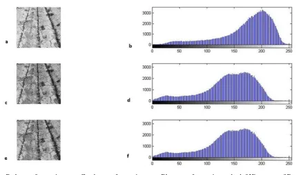
Figure 1. a. intensity part c. blue intesity e. red intesity information in YCbCr color space andb, d, and f were their histograms
Gray scale images
Conventional gray scale in most image programing algorithms is calculated by summing equal portion of red, green and blue colors ( 0.33×R+0.33×G+0.33×B). As it could been seen in the figure 2.
be seen from figure3. Plants' shad and soil track had a gray value to plant and certainly would be mixed with plant section of the images. Figure 1.b shows histogram of the figure 1.a., there are not clear and separate peaks in the histogram. As it was mentioned in methods, Otsu automatic thresholding method was used for thresholding. For the best thresholding process, clear peaks were necessary, so this gray scale images were not a suitable choice. it does not need any time for the color space conversion and it was this type's advantage.
RGB color space intensities
Then each RGB color space parts, means R, G and B were considered for the remainder of the image processing. Time cost for these color part separation was so little (0.0005-0.001 s) (figures 2.a, 2.c, 2. e). The G part related to green color (figure 2.c) was expected to show better results in comparison with other parts.
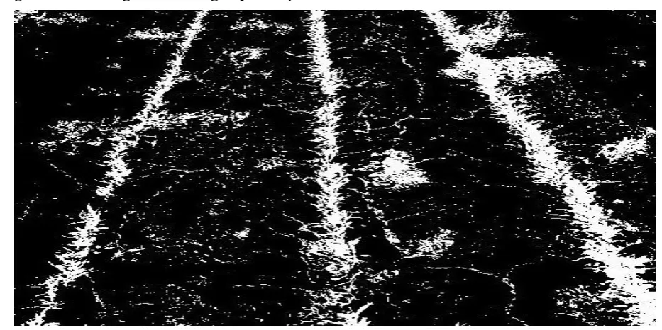
Figure 3. a. Red part of space image c. Greeb part of soace image e. Blue part of space image b, d, f Histogram of R, G and B parts
This color part showed better results in comparision with gray scale space, because plant sections were seen in better discrimination from soil and other background objects. But as it could be seen in the figure 2.c wet soil sections had a intensity value close to plant sections and was not vanished in soil.
RGB converted to greenness intensity
Figure 4. a. Converted image by greeness conversion b. Greeness image histogram
This better discrimination could be seen in figure 3.a. Figure 3.b showed that all gray value of pixels related to soil was converted to zero, so we had two separated peak that one of them had value of 0 and all remainder in the histogram was related to plant. So thresholding process could be performed so easily, because threshold value could be considered with values of a number close to 1 or so a little greater than 1. Figure 4 shows segmented image by this space.
Figure 5. Thresholded image
Figure 6. Filtered images and improved image
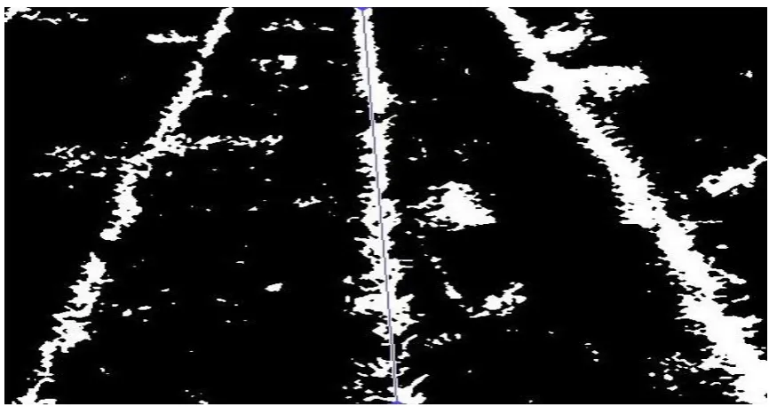
After filtering and deleting noise from images, Hough transform was used to find the row (Figure 7).
Figure 7 . Detected row by hough transform
Figure8 . Image after deleting plant section
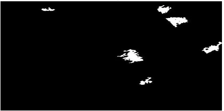
Then every spot of the image was numbered, and each spots' area were calculated, and small spots were omitted and center of the remainder were obtained (Figure 8).
Figure 9. image after omitting small spots
Center points coordinates then sent to developing board that it transferred information to determine what time the control system relay should be opened.
DISCUSSION
density that resulted in fuel valve being open for long time. The thermocouple closer to burner was more influenced by flames and temperature raise was more insignificant. The thermocouple near the outcome was under new air and wind impression and less in touch with flames. Counting of weeds in marked areas demonstrated that machine was available of destroying almost every small weed. The bigger weeds defoliation was considered as the factor of controlling unwanted plants. For broad leafed weeds number of leaves disappeared after 5 and 15 days were measured. After 5 days 78, 64, 56 and 37 percentages were disappeared or injured at 4, 8, 12, 16 kmh-1 respectively. The weeds injury after 15 days was 96, 87, 81 and 64 percentages at 4, 8, 12 and 16 kmh-1, respectively. Having fuel consumption under consideration and compromising with an approved weeding, an 8 to 12 km h-1 would give an acceptable result.
REFERENCES
Ascard J. 1994. Dose-response model for flame weeding in relation to plant size and density. Weed Research 34, 377-385.
Ascard J. 1995. Effects of flame weeding on weed species at different developmental stages, Weed Research 35, 397-411.
Ellwanger T C, Bingham J r ,Chappell W E. 1973. Physiological effects of ultra-high temperatures on corn. Weed Science 21, 266-269.
Lague C, GilJ l, Lehoux N, Pel oquin G. 1997. Engineering performances of propane flamers used for weed, insect pest, and plant disease control. Applied Engineering in Agriculture 13: 7-16.
Lampkin N. 1990. Organic Farming, Farming Press Books, Ipswich, UK.
Rahkonen J, Pietikanien J, Jokela H. 1999. The effects of flame weeding on soil microbal biomass. Biological Agriculture and Horticulture 16, 363-368.
Rifai M N. 1994. Flame and mechanical cultivation for weeds in Nova Scotia. In: The Technical Workshop of the Atlantic Committee in Agricultural Engineering, Fredericton, New Brunswick