© Universiti Tun Hussein Onn Malaysia Publisher’s Office
IJIE
Journal homepage: http://penerbit.uthm.edu.my/ojs/index.php/ijie
The International
Journal of
Integrated
Engineering
ISSN : 2229-838X e-ISSN : 2600-7916Solving for an Optimal Batch Size for a Single Machine Using
the Closed-form Equations to Minimize Inventory Cost
Athapol Ruangkanjanases
1*, Nithiphong Vikitset
2 1Chulalongkorn Business SchoolChulalongkorn University, Bangkok 10330, THAILAND
2TPI Polene Public Company Limited, Bangkok 10120, THAILAND
*Corresponding Author
DOI: https://doi.org/10.30880/ijie.2019.11.05.027
Received 25 April 2019; Accepted 08 September 2019; Available online 10 September 2019
1. Introduction
In the manufacturing system, batch sizing strategy has significant impacts on the production performance. The process with large batches usually has long lead time and large amount of finished goods inventory which incurs high inventory cost. Significant costs of inventory model are holding cost and setup cost [1].
Numbers of studies in the past offered the approaches to find the optimal batch size that improves manufacturing efficiency such as minimizing costs, minimizing production lead time, and maximizing service quality.
The approach to find the optimal batch size that minimized the total costs of raw materials ordering and finished goods inventory was developed by Parija and Sarker [2]. However, the cycle time interval between shipments or time intervals are fixed. Wang and Chen [3] proposed the new approach by modifying the cost function of Parija and Sarker to find the possible solutions. The simulation model in the supply chain system was applied to estimate the optimal batch size. Bertrand [4] published his development by extending the queuing model as well as the economic order quantity (EOQ) to find the optimal batch size in “made-to-stock” manufacturing system. However, the algorithm is an iterative procedure that the batch size is determined by adjusting the parameters for each iteration. The parameters were idle cost, wait time, production rates, in process inventory cost, and work orders. Wang and Sarker [5] published an article in which
Abstract: Batch sizing strategy in the manufacturing system has significant impacts on the manufacturing performance. In the previous research studies, researchers proposed complicated techniques such as optimization models, queuing theory, simulation, and complex algorithms to solve for the optimal batch size to increase the production efficiency. Using those techniques are difficult for plant managers to calculate for the optimal batch size. Therefore, the closed-form optimal batch size equations are proposed to minimize inventory cost of 2 models. The first model is illustrated when the inventory cost is associated with holding cost but without setup cost. The second model is illustrated when inventory cost is associated with both holding cost and setup cost. Besides the optimal batch size calculation, the value of λ, which is the shadow price of the available setup time, is also solved for sensitivity analysis purpose. Application of the closed-form equation is provided with various parameters applied to different products. The results show that the proposed closed-form equations approach performs well and verifies the effectiveness of the approach.
they applied mixed integer nonlinear programming in the Kanban System with the objective to determine the optimal batch size. The model to optimize batch size for an imperfect production system with quality assurance and rework was the developed by Ojha et al. [6]. A total cost equation was developed for the model, and the optimal ordering quantities were evaluated. In a study conducted by Rau and OuYang [7], it was found that the joint total costs incurred by the vendor and the buyer could be minimized by using an optimal batch size for integrated production–inventory policy in a supply chain system. Sohner and Schneeweiss [8] introduced the approach of hierarchically integrated lot size optimization. The approach was computational feasible and, based on some numerical results, was compared with a deterministic multi level capacitated lot sizing model.
Shin et al. [9] proposed a stochastic model to solve for the optimal batch size with process and product variability. Millar and Yang [10] applied queueing network model to investigate the potential of batch sizing as a control variable for lead time performance. They also used discrete optimization via marginal analysis to solve the nonlinear batch sizing problem. Koo et al. [11] introduced a linear search algorithm to find the optimal throughput rate and the batch size at a bottle neck machine. Lately, Wang et al. [12] proposed the chaotic-search-based self-organizing optimization approach to optimize the multistage batch scheduling problem. Yang et al. [13] applied iterative particle swarm optimization algorithm to solve for the batching optimization. Cheng et al. [14] improved ant colony optimization method to solve for the integrated scheduling of production and distribution with the objective to minimize cost.
Literature reviews show that the techniques explained above need a customization when production factors such as demands and capacity change. It is also difficult for a plant manager to customize the model when producing more than one type of products in a single machine. Therefore, this research article presents a simple version of batch sizing model for a single process system that is easy to use. The objective is to derive a closed-form batch size equation that minimizes the overall inventory cost.
2.
Assumptions and Notations
In the present study a mathematical model is constructed based on the assumptions and notations as follows;
2.1
Assumption
There are 9 assumptions of the model as follows; 1) Demands are deterministic.
2) Demands are constant over the evaluation period.
3) If the demands are not constant during a long evaluation period, the evaluation period can be divided into many smaller periods. Each period has individual constant demands but not necessary be the same rate among different intervals. Therefore, the optimal batch size equation could be independently applied to each small period.
4) Setup time is deterministic.
5) Setup time is an independent variable. In other words, set up time does not depend on what has been made before. 6) There are no maximum limits on batch size.
7) There are no minimum limits on batch size. 8) There are no integrality restrictions. 9) There are no non-negative restrictions.
2.2
Notations
Sets
𝒜𝒜 = Set of all items
ℛ = Set of items that require setup costs.
ℛ′= Set of items that do not require setup costs.
Note ℛ⋃ℛ′≡𝒜𝒜
Coefficients and parameters
C𝑖𝑖 = Setup cost of producing one batch of item i
h𝑖𝑖
=
Holding cost of the batch of item i in the evaluationperiod
𝐷𝐷𝑖𝑖 = Total demand for item i
𝒟𝒟 = Total demand of all items (𝒟𝒟=∑𝑖𝑖∈𝒜𝒜𝐷𝐷𝑖𝑖)
𝑝𝑝𝑖𝑖 = Processing time per unit of item i
𝑠𝑠𝑖𝑖 = Setup time per batch of item i
𝓢𝓢 = Available setup time
Decision variables
𝐵𝐵𝑖𝑖 = Batch size of item i
𝑛𝑛𝑖𝑖 = Total number of batches of item i required to produce Di units.
Note: 𝑛𝑛𝑖𝑖=𝐷𝐷𝐵𝐵𝑖𝑖𝑖𝑖 and 𝐵𝐵𝑖𝑖=𝐷𝐷𝑛𝑛𝑖𝑖𝑖𝑖
3.
Proposed Optimal Batch Size Equations
In this study, two types of objectives for batch sizing are proposed as follows;
1) The batch size equations that minimizes total inventory cost when associated with only holding cost (a model without setup cost).
2) The batch size equations that minimizes total inventory cost when associated with both holding cost and setup cost. The batch size equations for the first model are closed-form equations. In the second model, the problem is similar to the conventional Economic Order Quantity (EOQ) model where the total inventory cost consists of holding cost and setup cost. However, the optimal batch size is calculated based on the objective function and subjected to a capacity constraint. Although, there is no simple closed-form formula for this variation, a simple line search procedure is used to solve for the solution.
3.1 Optimal batch size equation to minimize total cost when associated with only holding cost
(a model without setup cost)
3.1.1 Explanation of the model
If the objective is to minimize the total holding cost or finished goods inventory value, the cost function that increases as the batch size increases must be included in the objective function. If 𝐵𝐵𝑖𝑖 is the feasible batch size, the term 𝐵𝐵𝐷𝐷𝑖𝑖𝑖𝑖 is cycle
time interval of item i as shown in (1)
𝐶𝐶𝐶𝐶𝐶𝐶𝑖𝑖=𝐷𝐷𝐵𝐵𝑖𝑖
𝑖𝑖 (1)
It implies the length of time that batch size Bi can supply the demand. The average finished goods inventory cost per batch is shown in (10) which is half of batch size times holding cost per CTI.
𝐴𝐴𝐴𝐴𝐴𝐴𝐴𝐴𝐴𝐴𝐴𝐴𝐴𝐴ℎ𝑜𝑜𝑜𝑜𝑜𝑜𝑜𝑜𝑛𝑛𝐴𝐴𝑐𝑐𝑜𝑜𝑠𝑠𝑐𝑐𝑝𝑝𝐴𝐴𝐴𝐴𝑏𝑏𝐴𝐴𝑐𝑐𝑐𝑐ℎ= 12·𝐵𝐵𝑖𝑖2·ℎ𝑖𝑖
𝐷𝐷𝑖𝑖 (2)
Therefore, total inventory cost per time T is number of cycles or number of batches per time T multiplies by the average holding cost per batch as shown in (3).
𝐶𝐶𝑜𝑜𝑐𝑐𝐴𝐴𝑜𝑜ℎ𝑜𝑜𝑜𝑜𝑜𝑜𝑜𝑜𝑛𝑛𝐴𝐴𝑐𝑐𝑜𝑜𝑠𝑠𝑐𝑐=12·𝐵𝐵𝑖𝑖2·ℎ𝑖𝑖
𝐷𝐷𝑖𝑖 ·𝑛𝑛𝑖𝑖=
1
2·
𝐵𝐵𝑖𝑖2·ℎ𝑖𝑖
𝐷𝐷𝑖𝑖 ·
𝐷𝐷𝑖𝑖
𝐵𝐵𝑖𝑖 =
1
2·𝐵𝐵𝑖𝑖·ℎ𝑖𝑖=
𝐷𝐷𝑖𝑖·ℎ𝑖𝑖
2·𝑛𝑛𝑖𝑖 (3)
Instead of using only holding cost, the penalty cost associated with the size of the batch may be used if the objective is to minimize finished goods inventory value. The items with high penalty cost will be produce in small batches that yield relatively short lead time and low inventory cost. For simplicity, only holding cost is used in this study.
The objective function and constraint are defined in (4) and (5), respectively.
𝑀𝑀𝑜𝑜𝑛𝑛 ∑ 𝐷𝐷𝑖𝑖·ℎ𝑖𝑖
2·𝑛𝑛𝑖𝑖
𝑖𝑖∈𝒜𝒜 (4)
𝑆𝑆𝑆𝑆𝑏𝑏𝑆𝑆𝐴𝐴𝑐𝑐𝑐𝑐𝑐𝑐𝑜𝑜 ∑𝑖𝑖∈𝒜𝒜𝑛𝑛𝑖𝑖·𝑠𝑠𝑖𝑖≤ 𝒮𝒮 (5)
Since there is only one constraint, this problem is solved by using Lagrangian relaxation technique [15]. The Lagrangian equation (L) is defined in (6) which yields λ, the total number of batches of item i (𝑛𝑛𝑖𝑖) and the optimal batch
size of item i as shown in (7), (8), and (9).
𝐿𝐿= ∑ 𝐷𝐷𝑖𝑖·ℎ𝑖𝑖
2·𝑛𝑛𝑖𝑖
𝑖𝑖∈𝒜𝒜 +𝜆𝜆· [(∑𝑖𝑖∈𝒜𝒜𝑛𝑛𝑖𝑖·𝑠𝑠𝑖𝑖)− 𝒮𝒮] (6)
𝜆𝜆=2·1𝒮𝒮2·�∑𝑖𝑖∈𝒜𝒜�𝐷𝐷𝑖𝑖·ℎ𝑖𝑖·𝑠𝑠𝑖𝑖�
2
𝑛𝑛𝑖𝑖=∑𝑖𝑖∈𝒜𝒜�𝐷𝐷𝒮𝒮𝑖𝑖·ℎ𝑖𝑖·𝑠𝑠𝑖𝑖·�𝐷𝐷𝑖𝑖𝑠𝑠·𝑖𝑖ℎ𝑖𝑖 (8)
𝐵𝐵𝑖𝑖= ∑𝑖𝑖∈𝒜𝒜�𝐷𝐷𝒮𝒮𝑖𝑖·ℎ𝑖𝑖·𝑠𝑠𝑖𝑖·�𝐷𝐷ℎ𝑖𝑖∙𝑠𝑠𝑖𝑖
𝑖𝑖 (9)
The derivation and FOC is illustrated in Appendix 1. The λ value from solving the Lagrangian equation implies the
impact of overall processing time reduction to total holding cost. The sensitivity analysis is widely used to measure the impacts of fluctuations in parameters of a mathematical model or system on the outputs or performance of the system [16, 17].
The λ in (7) is the dual variable. It can be interpreted as a “shadow price” of the available setup time. For example, if the value of λ is 25, it implies that the inventory cost will be reduced by 25 dollars when the available setup time is increased by 1 hour.
This λ is always positive since it is always cheaper to produce in smaller batches, unless there are costs associated
with number of batches.
3.1.2 Numerical Illustration
To illustrate how to apply equation (8) and (9), an example of scenario is setup. Assume that there are 5 products; A, B, C, D, and E, to be produced. Processing time for each unit of A, B, C, D, and E are 0.25, 1.25, 1.8, 0.5, and 2 hours respectively. The machine requires 20 hours for a setup before it can produce product A. Setup times for product B, C, D, and E are 30, 15, 25, and 20. The annual demands are 258, 1,105, 1,126, 1,130, and 500 units for product A, B, C, D, and E respectively. The holding cost per unit per year for each product is also shown in Table 1.
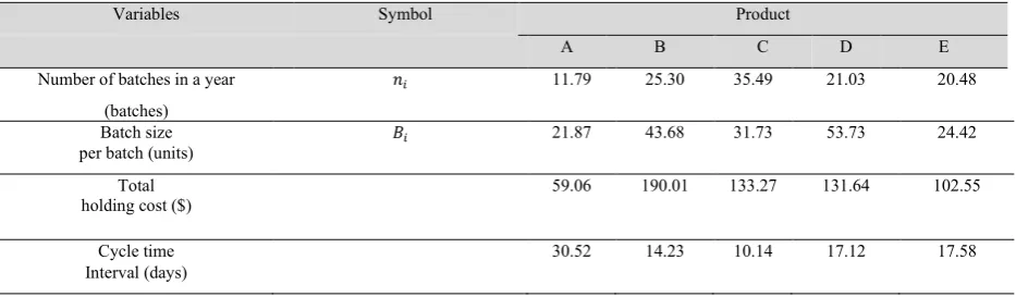
All data in Table 1 is then be used. Total processing time required to produce all products is calculated as shown. (0.25)(258) + (1.25)(1,105) + (1.8)(1,126) + (0.5)(1,130) + (2)(500) = 5,037.55 hours. If the available machine hours in a year are 7,500 hours and total processing hours (without setup time) are 5,037.55 hours, the available setup time is 7,500 – 5037.55 = 2,462.45 hours. Therefore, using 𝓢𝓢 =2,462.45 in equation (8) and (9), the number of batches (n) and batch sizes (B) can be calculated. The total holding cost and the cycle time interval for each product are also summarized in Table 2.
The λ value for this instance is 0.25. This implies that if total processing time has been reduced by 1 hour that is equivalent to adding 1 hour to the available setup time, total inventory cost will be reduced by $0.25.
Table 1 Production parameters
Variables Symbol Product
A B C D E
Processing time 𝑝𝑝𝑖𝑖 0.250 1.250 1.800 0.500 2.000
per unit (hours)
Setup time 𝑠𝑠𝑖𝑖 20.00 30.00 15.00 25.00 20.00
per batch (hours)
Annual demand 𝐷𝐷𝑖𝑖 258.0 1105 1126 1130 500
(units)
Holding Cost h𝑖𝑖 5.40 8.70 8.40 4.90 8.40
per unit/year ($)
Table 2 Results of optimal batch sizes that minimize inventory cost for a model with holding cost but without setup cost
Variables Symbol Product
A B C D E
Number of batches in a year 𝑛𝑛𝑖𝑖 11.79 25.30 35.49 21.03 20.48
(batches)
Batch size 𝐵𝐵𝑖𝑖 21.87 43.68 31.73 53.73 24.42
per batch (units)
Total
holding cost ($) 59.06 190.01 133.27 131.64 102.55
Cycle time 30.52 14.23 10.14 17.12 17.58
3.2 Optimal batch size equations to minimize total cost when associated with both holding cost
and setup cost
3.2.1 Explanation of the model
The optimal batch size with setup costs is similar to economic order quantity (EOQ) except for the capacity constraint is added to the problem. Setup cost is the cost of initializing each batch production such as cleaning chemical, electricity used to warm up the machine, or the replacement of non-reusable molds. In addition, setup cost can also be interpreted as the ordering cost of raw materials from the supplier if company wants to use “Just-In-Time” (JIT) inventory management on that batch production. Theoretically, using JIT will not incur the holding cost for raw material. Raw materials will be delivered just before that batch starts. If the company wants to use JIT for all batches, total number of orders from the supplier will be the same as total number of batches; therefore, the ordering cost can be considered as part of the setup cost. For simplicity in this study, the proposed model does not separate setup cost into ordering cost and initializing cost. It will be defined as fixed cost of producing one batch.
When producing multiple products, some products may require both holding cost and setup cost while some only require holding cost. Therefore, the production plan is divided into two sets; (i) the items that incur setup cost and holding cost for each batch produced and (ii) the items that incur holding cost but do not incur setup cost for each batch. The objective function is to minimize total setup cost and total holding cost subjected to the total setup time spent cannot exceed the available setup time. The objective function and capacity constraint are defined (10) and (11), respectively.
𝑀𝑀𝑜𝑜𝑛𝑛 ∑ �12·𝐷𝐷𝑖𝑖·ℎ𝑖𝑖
𝑛𝑛𝑖𝑖 +𝐶𝐶𝑖𝑖·𝑛𝑛𝑖𝑖�
𝑖𝑖∈ℛ +∑𝑖𝑖∈ℛ′�12·𝐷𝐷𝑛𝑛𝑖𝑖·𝑖𝑖ℎ𝑖𝑖� (10)
𝑆𝑆𝑆𝑆𝑏𝑏𝑆𝑆𝐴𝐴𝑐𝑐𝑐𝑐𝑐𝑐𝑜𝑜 ∑𝑖𝑖∈𝐴𝐴𝑛𝑛𝑖𝑖·𝑠𝑠𝑖𝑖≤ 𝒮𝒮 (11)
Like the previous model, Lagrangian relaxation technique is used to solve the problem. The Lagrangian equation of this problem is defined in (12).
𝐿𝐿= ∑ �12·𝐷𝐷𝑖𝑖·ℎ𝑖𝑖
𝑛𝑛𝑖𝑖 +𝐶𝐶𝑖𝑖·𝑛𝑛𝑖𝑖�
𝑖𝑖∈ℛ +∑𝑖𝑖∈ℛ′�12·𝐷𝐷𝑛𝑛𝑖𝑖·ℎ𝑖𝑖𝑖𝑖�+𝜆𝜆· (∑𝑖𝑖∈𝐴𝐴𝑛𝑛𝑖𝑖·𝑠𝑠𝑖𝑖− 𝒮𝒮) (12)
First order conditions for minimizing the Lagrangian equation are defined in (13), (14), and (15), respectively.
𝜕𝜕𝜕𝜕
𝜕𝜕𝑛𝑛𝑖𝑖=−
1
2·
𝐷𝐷𝑖𝑖·ℎ𝑖𝑖
𝑛𝑛𝑖𝑖2 +𝐶𝐶𝑖𝑖+𝜆𝜆·𝑠𝑠𝑖𝑖= 0 ∀𝑜𝑜 ∈ ℛ (13)
𝜕𝜕𝜕𝜕
𝜕𝜕𝑛𝑛𝑖𝑖=−
1
2·
𝐷𝐷𝑖𝑖·ℎ𝑖𝑖
𝑛𝑛𝑖𝑖2 +𝜆𝜆·𝑠𝑠𝑖𝑖= 0 ∀𝑜𝑜 ∈ ℛ′ (14)
𝜕𝜕𝜕𝜕
𝜕𝜕𝜕𝜕=∑𝑖𝑖∈𝐴𝐴𝑛𝑛𝑖𝑖·𝑠𝑠𝑖𝑖− 𝒮𝒮= 0 (15)
From (13) and (14),
𝑛𝑛𝑖𝑖=�2·(𝐶𝐶𝐷𝐷𝑖𝑖𝑖𝑖+𝜕𝜕·ℎ𝑖𝑖·𝑠𝑠𝑖𝑖) ∀𝑜𝑜 ∈ ℛ (16)
𝑛𝑛𝑖𝑖=�2𝐷𝐷·𝑖𝑖𝜕𝜕·ℎ·𝑠𝑠𝑖𝑖𝑖𝑖 ∀𝑜𝑜 ∈ ℛ′ (17)
Then, substitute 𝑛𝑛𝑖𝑖 from (16) and (17) to (15).
�∑ � 𝐷𝐷𝑖𝑖·ℎ𝑖𝑖
2·(𝐶𝐶𝑖𝑖+𝜕𝜕·𝑠𝑠𝑖𝑖)+∑ �
𝐷𝐷𝑖𝑖·ℎ𝑖𝑖
2·𝜕𝜕·𝑠𝑠𝑖𝑖
𝑖𝑖∈ℛ′
𝑖𝑖∈ℛ �·𝑠𝑠𝑖𝑖− 𝒮𝒮= 0 (18)
Solving for λ from the above equation when ℛ≢𝜙𝜙is quite difficult; therefore, line search procedure is used to evaluate
the value of λ. If batches of all items incur setup costs and there is no positive value of λ that satisfies the equation, the capacity constraint is a non-binding constraint. Therefore, the problem can be solved like an unconstrained problem. That is, the first order condition is 𝜕𝜕𝜕𝜕
𝜕𝜕𝑛𝑛𝑖𝑖=−
1
2·
𝐷𝐷𝑖𝑖·ℎ𝑖𝑖
𝑛𝑛𝑖𝑖2 +𝐶𝐶𝑖𝑖= 0;∀𝑜𝑜 ∈ 𝐴𝐴
;
which is equivalent to the classical EOQ. Solving the𝑛𝑛𝑖𝑖=�𝐷𝐷2𝑖𝑖·𝐶𝐶ℎ𝑖𝑖𝑖𝑖 (19)
𝐵𝐵𝑖𝑖=�2·𝐶𝐶ℎ𝑖𝑖𝑖𝑖·𝐷𝐷𝑖𝑖 (20)
Conversely, if batches of some items do not require setup costs and available setup time is positive, there is a positive
value of λ that satisfies the equation. The proof of this is shown in Appendix 2.
3.2.2 Numerical Illustration (
ℛ
≡
A)
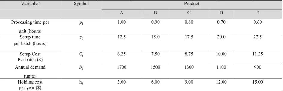
To illustrate how to apply equation (19) and (20), an example of scenario is setup. Assume that there are 5 products; A, B, C, D, and E, to be produced. All products incur both holding cost and setup cost. The annual demands and production requirements are given in Table 3.
Table 3 The annual demand and production requirements for the model with holding cost and setup cost.
Variables Symbol Product
A B C D E
Processing time per 𝑝𝑝𝑖𝑖 1.00 0.90 0.80 0.70 0.60
unit (hours)
Setup time 𝑠𝑠𝑖𝑖 12.5 15.0 17.5 20.0 22.5
per batch (hours)
Setup Cost C𝑖𝑖 6.25 7.50 8.75 10.00 11.25
Per batch ($)
Annual demand 𝐷𝐷𝑖𝑖 1700 1500 1300 1100 900
(units)
Holding cost h𝑖𝑖 3.00 6.00 9.00 12.00 15.00
per year ($)
Total processing time required to produce all items are 5,400 hours. If there are 7,500 hours available in a year, the factory will have 2,100 hours available for total setup time.
Since all products incur both holding cost and setup cost the initial value of λ is set to zero because it can be checked whether the constraint is binding or not. The line search procedure then be used to solve the problem. This line search procedure is based on the first order approximation. We estimate the first order derivative by perturbing the value of λ in
(18). Then we approximate the new value of λ that makes (18) zero from its first derivative. Equation (18) will converge
to zero in finite steps since its limit approaches zero when λ approaches infinity.
Case:ℛ ≡ 𝐴𝐴 (all products incur both holding cost and setup cost)
Let
𝑍𝑍[𝜆𝜆(𝑘𝑘)] =�∑ � 𝐷𝐷𝑖𝑖·ℎ𝑖𝑖
2·(𝐶𝐶𝑖𝑖+𝜕𝜕·𝑠𝑠𝑖𝑖)
𝑖𝑖∈ℛ �·𝑠𝑠𝑖𝑖− 𝒮𝒮 (21)
𝑌𝑌=𝑍𝑍[𝜕𝜕𝜕𝜕((𝑘𝑘+1𝑘𝑘+1)])−𝜕𝜕−𝑍𝑍([𝜕𝜕𝑘𝑘)(𝑘𝑘)] (22)
Where k = number of iterations
Y = rate of change of function Z respect to the change in λ value.
Initialization step:
1. Set λ(0) = 0 and 𝑍𝑍(0) =∑ �𝐷𝐷𝑖𝑖·ℎ𝑖𝑖
2·𝐶𝐶𝑖𝑖 ·𝑠𝑠𝑖𝑖
𝑚𝑚
𝑖𝑖=1 − 𝒮𝒮
2. If Z ≤ 0, the constraint is nonbinding. The optimal number of batches and batch size are 𝑛𝑛𝑖𝑖=�𝐷𝐷2𝑖𝑖·𝐶𝐶ℎ𝑖𝑖
𝑖𝑖and𝐵𝐵𝑖𝑖=
𝐷𝐷𝑖𝑖
𝑛𝑛𝑖𝑖, respectively.Otherwise, set k = 1 and λ(k) = small positive number. Go to main step.
1. Evaluate function Z(k) and Y.
2. If Z(k) < 0, set λ(1) to a smaller number and repeat the initialization steps.
3. If Z(k) ≤ ε; where, ε = small positive number close to zero, then stop. The optimal λ = λ(k).
4. k = k + 1
5. 𝜆𝜆(𝑘𝑘) = 𝜆𝜆(𝑘𝑘 −1)−𝑍𝑍𝑌𝑌((𝑘𝑘−1𝑘𝑘−1))
6. Repeat main steps.
The optimal number of batches is
𝑛𝑛𝑖𝑖=�2·(𝐶𝐶𝐷𝐷𝑖𝑖𝑖𝑖+𝜕𝜕·ℎ𝑖𝑖·𝑠𝑠𝑖𝑖); ∀𝑜𝑜 ∈ 𝐴𝐴 (23)
And the optimal batch size is
𝐵𝐵𝑖𝑖=𝐷𝐷𝑛𝑛𝑖𝑖
𝑖𝑖; ∀𝑜𝑜 ∈ 𝐴𝐴. (24)
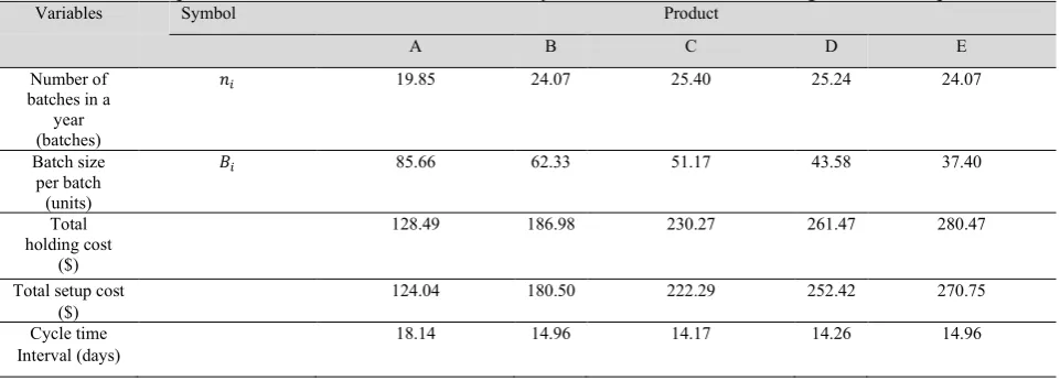
The line search procedure is summarized in Table 4. The value of function Z(λ = 0) > 0 indicates that the capacity
constraint of the original problem is binding constraint. In other words, all available setup time will be used and there exists a positive value of optimal λ; for this instant, the optimal λ = 0.017943. Using the optimal batch size equation in (24) and λ = 0.017943, the optimal batch sizes and other parameters then be calculated and shown in Table 5.
Table 4 Line search procedure
Iteration λ Z(λ) Y
Initialization 0 37.34867 -
1 0.01 16.29054 -2,105.81
2 0.017736 0.42028 -2,051.49
3 0.017941 0.00484 -2,027.86
4 0.017943 0
Table 5 Results of optimal batch sizes that minimize inventory cost for a model with holding cost and setup cost
Variables Symbol Product
A B C D E
Number of batches in a
year
𝑛𝑛𝑖𝑖 19.85 24.07 25.40 25.24 24.07
(batches)
Batch size 𝐵𝐵𝑖𝑖 85.66 62.33 51.17 43.58 37.40
per batch (units)
Total
holding cost 128.49 186.98 230.27 261.47 280.47
($)
Total setup cost 124.04 180.50 222.29 252.42 270.75
($)
Cycle time 18.14 14.96 14.17 14.26 14.96
Interval (days)
4.
Application and Results
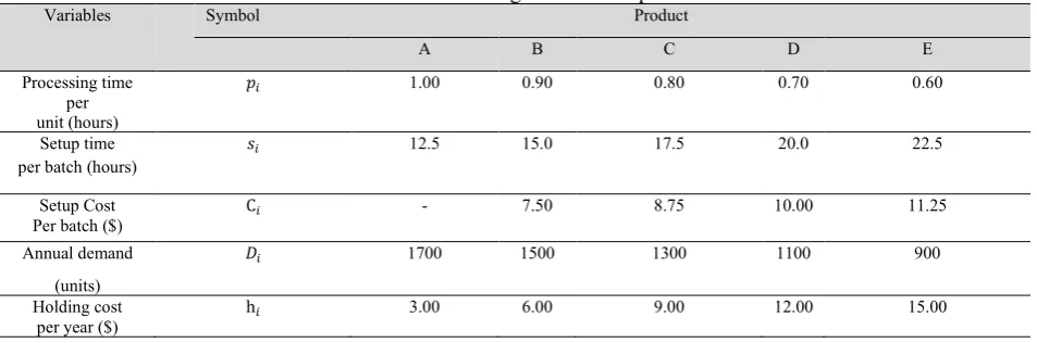
When applying the closed-form batch size equations in real situations, the problem occurs when producing multiple products and some products incur both holding cost and set up cost while some products incur only holding cost (ℛ´ ≢ 𝜙𝜙). This situation makes the problem more complicated. An example of the case is shown in Table 6. Product A only incurs holding cost but does not incur setup cost while other products incur both holding cost and setup cost.
The line search procedure is performed slightly different from the previous example. We cannot set λ to zero because
This line search procedure is based on the first order approximation. We estimate the first order derivative by
perturbing the value of λ in (18). Then we approximate the new value of λ that makes (18) zero from its first derivative. Equation (18) will converge to zero in finite steps since its limit approaches zero when λ approaches infinity.
Table 6 The annual demand and production requirements when some products incur only holding cost while some incurs both holding cost and setup cost
Variables Symbol Product
A B C D E
Processing time
per 𝑝𝑝𝑖𝑖 1.00 0.90 0.80 0.70 0.60
unit (hours)
Setup time 𝑠𝑠𝑖𝑖 12.5 15.0 17.5 20.0 22.5
per batch (hours)
Setup Cost C𝑖𝑖 - 7.50 8.75 10.00 11.25
Per batch ($)
Annual demand 𝐷𝐷𝑖𝑖 1700 1500 1300 1100 900
(units)
Holding cost h𝑖𝑖 3.00 6.00 9.00 12.00 15.00
per year ($)
Case:ℛ′≢ ∅
Let
𝑍𝑍[𝜆𝜆(𝑘𝑘)�∑ � 𝐷𝐷𝑖𝑖·ℎ𝑖𝑖
2·(𝐶𝐶𝑖𝑖+𝜕𝜕·𝑠𝑠𝑖𝑖)∑ �
𝐷𝐷𝑖𝑖·ℎ𝑖𝑖
2·𝜕𝜕·𝑠𝑠𝑖𝑖
𝑖𝑖∈ℛ′
𝑖𝑖∈ℛ �·𝑠𝑠𝑖𝑖− 𝒮𝒮 (25)
𝑌𝑌
=
𝑍𝑍[𝜕𝜕𝜕𝜕((𝑘𝑘+1𝑘𝑘+1)])−𝑍𝑍−𝜕𝜕([𝑘𝑘𝜕𝜕()𝑘𝑘)] (26)Where k = number of iterations
Y = rate of change of function Z with respect to the change in λ value.
Initialization step:
1. Set λ(0) = small positive number and λ(1) = small positive number slightly larger than λ(0)
2. Set k = 1 and go to the main step.
Main step:
1. Evaluate function Z(k) and Y.
2. If Z(k) < 0, repeat the initialization steps and set λ(0) to a smaller number.
3. If Z(k) ≤ ε; where, ε = small positive number close to zero, then stop. The optimal λ = λ(k).
4. k = k + 1
5. 𝜆𝜆(𝑘𝑘) = 𝜆𝜆(𝑘𝑘 −1)−𝑍𝑍𝑌𝑌((𝑘𝑘−1𝑘𝑘−1))
6. Repeat main step.
The optimal number of batches is
𝑛𝑛𝑖𝑖=�2·(𝐶𝐶𝐷𝐷𝑖𝑖·ℎ𝑖𝑖
𝑖𝑖+𝜕𝜕·𝑠𝑠𝑖𝑖);∀𝑜𝑜 ∈ ℛ (27)
And
𝑛𝑛𝑖𝑖=�2𝐷𝐷·𝑖𝑖𝜕𝜕··ℎ𝑠𝑠𝑖𝑖𝑖𝑖;∀𝑜𝑜 ∈ ℛ′. (28)
𝐵𝐵𝑖𝑖=𝐷𝐷𝑛𝑛𝑖𝑖
𝑖𝑖; ∀𝑜𝑜 ∈ 𝐴𝐴 (29)
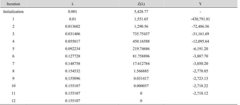
Therefore, the initial value of λ is set to 0.001. Using line search procedure, λ converges to the optimal value in 12 iterations as shown in Table 7.
The optimal solutions then be calculated as shown in Table 8. The numbers may not be integer but they provide the lower bound of the parameters.
Table 7 Line search procedure (case: ℛ´ ≢ 𝜙𝜙)
Iteration λ Z(λ) Y
Initialization 0.001 5,428.77 -
1 0.01 1,551.65 -430,791.81
2 0.013602 1,290.56 -72,486.56
3 0.031406 735.75437 -31,161.69
4 0.055017 450.16588 -12,095.64
5 0.092234 219.74686 -6,191.20
6 0.127728 81.758896 -3,887.70
7 0.148758 17.612784 -3,050.20
8 0.154532 1.566885 -2,778.85
9 0.155096 0.031417 -2,723.13
10 0.155107 0.000057 -2,718.22
11 0.155107 0 -2,718.12
12 0.155107 0
Table 8 Results of optimal batch sizes that minimize inventory cost (case: ℛ´ ≢ 𝜙𝜙) Variables Symbol Product
A B C D E
Number of batches in a
year
𝑛𝑛𝑖𝑖 36.27 21.40 22.59 22.44 21.40
(batches)
Batch size 𝐵𝐵𝑖𝑖 46.88 70.09 57.55 49.01 42.06
per batch (hours)
Total
holding cost 70.31 210.28 258.97 294.06 315.43
($)
Total setup cost - 160.50 197.66 224.44 240.74
($)
Cycle time 9.93 16.82 15.94 16.04 16.82
Interval (days)
5.
Conclusion
The closed-form optimal batch size equations are proposed to minimize inventory cost of 2 models. The first model is illustrated when the inventory cost is associated with holding cost but without setup cost. The second model is illustrated when inventory cost is associated with both holding cost and setup cost. The line search procedure are applied to solve for the optimal solutions in the second model. Besides the optimal batch size calculation, the advantage of this proposed closed-form equation is that the value of λ can also be solved for sensitivity analysis. The λ is interpreted as “shadow price” of the available setup time. It shows the amount of inventory cost saving when the available setup time is increased by 1 hour.
However, this research is just a starting point some of the questions are still remained. The optimal batch size with a different objective would change the solution. Since the optimal solutions from this approach may not be integer, future research could be involved with mixed integer programming.
Appendix
Appendix 1: Solving Lagrangian equation
𝐿𝐿= ∑ 𝐷𝐷𝑖𝑖·ℎ𝑖𝑖
2·𝑛𝑛𝑖𝑖
𝑖𝑖∈𝒜𝒜 +𝜆𝜆· [(∑𝑖𝑖∈𝒜𝒜𝑛𝑛𝑖𝑖·𝑠𝑠𝑖𝑖)− 𝒮𝒮]
First order conditions;
𝜕𝜕𝜕𝜕
𝜕𝜕𝑛𝑛𝑖𝑖=−
1
2·
𝐷𝐷𝑖𝑖·ℎ𝑖𝑖
𝑛𝑛𝑖𝑖2 +𝜆𝜆·𝑠𝑠𝑖𝑖= 0 ;𝑓𝑓𝑜𝑜𝐴𝐴𝐴𝐴𝑜𝑜𝑜𝑜𝑜𝑜𝑐𝑐𝐴𝐴𝑖𝑖𝑠𝑠 𝜕𝜕𝜕𝜕
𝜕𝜕𝜕𝜕= (∑𝑖𝑖∈𝒜𝒜𝑛𝑛𝑖𝑖·𝑠𝑠𝑖𝑖)− 𝒮𝒮= 0
Rearrange the first equation of FOC,
𝑛𝑛𝑖𝑖2=12 ·𝐷𝐷𝜆𝜆𝑖𝑖··𝑠𝑠ℎ𝑖𝑖 𝑖𝑖
Since n ≥ 0, substitute 𝑛𝑛𝑖𝑖=�12·𝐷𝐷𝜕𝜕𝑖𝑖··𝑠𝑠ℎ𝑖𝑖𝑖𝑖in the second equation of FOC and solve for λ;
𝜆𝜆=2·1𝒮𝒮2·�∑𝑖𝑖∈𝒜𝒜�𝐷𝐷𝑖𝑖·ℎ𝑖𝑖·𝑠𝑠𝑖𝑖�
2
Similar to the optimal λ in Appendix 1, optimal λ is always positive if at least one item requires holding cost and setup
time. This makes capacity constraint ∑𝑖𝑖∈𝒜𝒜𝑛𝑛𝑖𝑖·𝑠𝑠𝑖𝑖≤ 𝒮𝒮 binding constraint of ∑𝑖𝑖∈𝒜𝒜𝑛𝑛𝑖𝑖·𝑠𝑠𝑖𝑖= 𝒮𝒮.
Substitute 𝜆𝜆=2·1𝒮𝒮2·�∑𝑖𝑖∈𝒜𝒜�𝐷𝐷𝑖𝑖·ℎ𝑖𝑖·𝑠𝑠𝑖𝑖� 2
in the first equation of FOC and solve for ni,
𝑛𝑛𝑖𝑖= 𝒮𝒮
∑𝑖𝑖∈𝒜𝒜�𝐷𝐷𝑖𝑖·ℎ𝑖𝑖·𝑠𝑠𝑖𝑖
·�𝐷𝐷𝑖𝑖𝑠𝑠·ℎ𝑖𝑖
𝑖𝑖
And, minimum batch size for item i is𝐵𝐵𝑖𝑖= 𝐷𝐷𝑛𝑛𝑖𝑖
𝑖𝑖. Appendix 2: Proof
Ifℛ′≢ ∅𝐴𝐴𝑛𝑛𝑜𝑜𝒮𝒮> 0, there exists a positive value of λ that satisfies equation �∑ � 𝐷𝐷𝑖𝑖·ℎ𝑖𝑖
2·(𝐶𝐶𝑖𝑖+𝜕𝜕·𝑠𝑠𝑖𝑖)+∑ �
𝐷𝐷𝑖𝑖·ℎ𝑖𝑖
2·𝜕𝜕·𝑠𝑠𝑖𝑖
𝑖𝑖∈ℛ′
𝑖𝑖∈ℛ �·𝑠𝑠𝑖𝑖−
𝒮𝒮= 0
lim
𝜕𝜕→0+∑ �
𝐷𝐷𝑖𝑖·ℎ𝑖𝑖
2·(𝐶𝐶𝑖𝑖+𝜕𝜕·𝑠𝑠𝑖𝑖)⟶ ∑ �
𝐷𝐷𝑖𝑖·ℎ𝑖𝑖
2·𝐶𝐶𝑖𝑖
𝑖𝑖∈ℛ
𝑖𝑖∈ℛ
lim
𝜕𝜕→0+∑ �
𝐷𝐷𝑖𝑖·ℎ𝑖𝑖
2·𝜕𝜕·𝑠𝑠𝑖𝑖
𝑖𝑖∈ℛ′ ⟶ ∞
lim
𝜕𝜕→∞∑ �
𝐷𝐷𝑖𝑖·ℎ𝑖𝑖
2·(𝐶𝐶𝑖𝑖+𝜕𝜕·𝑠𝑠𝑖𝑖)⟶0
𝑖𝑖∈ℛ
Therefore, the range of �∑ � 𝐷𝐷𝑖𝑖·ℎ𝑖𝑖
2·(𝐶𝐶𝑖𝑖+𝜕𝜕·𝑠𝑠𝑖𝑖)+∑ �
𝐷𝐷𝑖𝑖·ℎ𝑖𝑖
2·𝜕𝜕·𝑠𝑠𝑖𝑖
𝑖𝑖∈ℛ′
𝑖𝑖∈ℛ �= (0,∞).
References
[1] Heizer, J., Render, B., and Munson, C. Operations Management Sustainability and Supply Chain Management. 12th
Edition, (2017), Pearson Education Limited, Essex, England
[2] Parija, G.R., Sarker, B.R. Operations Planning in a Supply Chain System with Fixed-interval Deliveries of Finished Goods to Multiple Customers. IIE Transactions, Volume 7, Number 14, (1999), pp. 157-163.
[4] Bertrand, J.W.M. Multiproduct Optimal Batch Sizes with In-process Inventories and Multi Work Centers. IIT Transaction, Volume 17, Number 2, (1985), pp. 157 – 163.
[5] Wang, S. and Sarker, B.R. A Single-stage Supply Chain System Controlled by Kanban under Just-in-time Philosophy. Journal of the Operational Research Society, Volume 55, (2004), pp. 485–494.
[6] Ojha, D., Sarker, B.R., and Biswas, P. An Optimal Batch Size for an Imperfect Production System with Quality Assurance and Rework. International Journal of Production Research, Volume 45, Number 14, (2007), pp. 3191-3214.
[7] Rau, H. and OuYang, B.C. An Optimal Batch Size for Integrated Production-inventory Policy in Supply Chain. European Journal of Operational Research. Volume 185, (2004), pp. 619-634.
[8] Sohner, V. and Schneeweiss, C. Hierarchically integrated lot size optimization. European Journal of Operational Research, Volume 86, Number 1, (1995), pp. 73-90.
[9] Shin, D., Park, J., Kim, N., and Wysk, R.A. A stochastic model for the optimal batch size in multi-step operations with process and product variability. International Journal of Production Research, Volume 47, Number 14, (2009), pp. 3919-3936.
[10]Millar, H. H., and Yang, T. Batch sizes and lead-time performance in flexible manufacturing systems. International Journal of Flexible Manufacturing Systems, vol. 8, no. 1, (1996), pp. 5-21.
[11]Koo, P. H., Bulfin, R., and Koh, S.G. Determination of batch size at a bottleneck machine in manufacturing systems. International Journal of Production Research, Volume 45, Number 5, (2007), pp. 1215-1231.
[12]Wang, G., Liang, T., and Song, W. A chaotic-search-based self-organizing optimization approach for multistage batch scheduling problem. Proceedings of the 32nd Chinese Control Conference, Xi'an, China, (2013), pp. 8441-8445.
[13]Yang, L., Pan, H. P., and Zhang, Y. B. Comprehensive optimization of batch process based on particle swarm optimization algorithm. Proceedings of the 29th Chinese Control and Decision Conference, Chongqing, China, (2017), pp. 4504-4508.
[14]Cheng, Y. B., Leung, J.Y.-T., and Li, K. Integrated scheduling of production and distribution to minimize total cost using an improved ant colony optimization method. Computers and Industrial Engineering, Volume 83, (2015), pp. 217-225.
[15]Calkin, M. G. Lagrangian and Hamiltonian Mechanics, World Scientific Publishing Co. Pte. Ltd., (1996), Singapore. [16]Senen, M. S., Mohamad, E. J., Mohamad Ameran, H. L., Rahim, R. A., Faizan, O. M., & Mohd Muji, S. Z.
Simulation Analysis of Dual Excitations Method for Improving the Sensitivity Distribution of an Electrical Capacitance Tomography System. International Journal of Integrated Engineering, Volume 9, Number 1, (2017), pp. 10-15.