CFD Simulation of Gas-Solid Two-Phase Flow in Pneumatic Conveying of Wheat

CFD Simulation of Gas-Solid Two-Phase Flow

in Pneumatic Conveying of Wheat

Sarrami Foroushani, Ali; Nasr Esfahany, Mohsen*

Department of Chemical Engineering, Isfahan University of Technology, Isfahan, I.R. IRAN

ABSTRACT: Computational Fluid Dynamics (CFD) simulations of gas-solid flow through a positive low-pressure pneumatic conveyor were performed using Eulerian-Eulerian framework. Pressure drop in pneumatic conveying pipelines, creation and destruction of plugs along the horizontal and vertical pipes, effect of 90° elbows and U-bends on cross-section concentrations, and rope formation and dispersion were numerically investigated for the wheat particles at ten different operating conditions. The effects of air inlet velocity and the conveying capacity on the flow behavior were also discussed. Both parameters played a significant role in the conveying flow pattern and also the pressure drop. The numerical simulations validated against the experimental data from literature and also qualitatively compared with trends in experimental data. Excellent quantitative agreement between experimental and simulated results (±1%) was observed in dense-phase conveying. For the dilute-dense-phase conveying simulations underestimated the values of pressure drop by 20%; however, this still falls within the acceptable error ranges reported in the literature. This study stresses the capability of CFD to explain and predict the behavior of complex gas-solid conveying systems and to be used productively for investigations in pneumatic conveying of agricultural and pharmaceutical particles as an aid in the system design..

KEY WORDS:Gas-solid two-phase flow; Pneumatic conveying; Computational fluid dynamics; U-bend, 90° elbow.

INTRODUCTION

Pneumatic conveying is a commonly used method for the transport of solid particles such as agricultural seeds, coal, lime, cement, granular chemicals, and plastic chips over distances up to several kilometers. When solid materials are transported in a pneumatic conveying system two basic modes of flow may be observed, namely: (1) dilute phase flow or suspension flow in which the conveying velocity is sufficient to keep particles suspended while moving through the pipeline, (2) dense phase flow or non-suspension flow in which

the conveying gas velocity is less than necessary to keep particles suspended so that majority of particles move along the pipe while they are not suspended in the conveying gas [1]. Investigators used different definitions to distinguish these two flow regimes [2,3]. Since conveyed materials have great influences on flow modes, authors such as Geldart, Molerus, Dixon, Pan [4] provided diagrams giving some indication of different particle flow modes based on the particle's properties (e.g., mean diameter, density) [3].

*To whom correspondence should be addressed. +E-mail:[email protected]

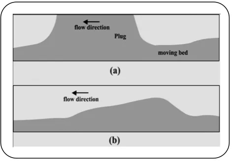
Fig. 1: (a) Plug flow. (b) Dune flow.

Regarding the dense phase pneumatic conveying of granular materials, flowing through a horizontal pipe, a wave-like flow has been observed which is shown in Fig. 1 [1]. In wave-like gas-solid flow, also referred to dune flow, materials picked up from a moving bed form a moving plug; then, dropped off toward the moving bed; having passed a distance along the pipe. If the rolling waves do not completely fill the pipe cross-section, the flow will be called dune flow to be more distinct. However, in the current paper, the wave-like flow is simply called plug flow. Dense phase flow pneumatic conveying attracts more interest in industrial applications due to lower rate of particle attrition and pipeline wear as well as high particle mass flow rates which leads to a reduction in need for the conveying gas to convey a special amount of particles and greater energy efficiency [1,5]. Since pneumatic conveying is associated with gas-solid two-phase flow, modeling of such systems is based on the approaches exist for two-phase flow modeling, i.e., Eulerian-Eulerian, Eulerian-Lagrangian and MP-PIC hybrid models. In Eulerian-Eulerian also referred to two-fluid approach, each phase is assumed to behave like a continuum. Separate sets of conservation equations are used for each phase; therefore, three additional equations governing the interfacial transfer of mass, momentum, and energy between phases are required to model the interactions between phases (jump conditions). In Eulerian-Lagrangian model also referred to as particle trajectory approach, solid particles are uncoupled from the continuous phase and the trajectories of many individual particles are calculated. In other words, in particle trajectory model an appropriate form of Newton's

second law plus an accurate solution of the fluid flow field are the governing equations while in two-fluid model the governing equations are the two separate sets of conservation equations plus jump conditions and closure relations [6]. The third method, MP-PIC, is a hybrid method where the gas-phase is treated as a continuum in the Eulerian framework and the solids are modeled in the Lagrangian framework via tracking particles. The MP-PIC method employs a fixed Eulerian grid, and Lagrangian parcels are used to transport mass, momentum, and energy through this grid in a way that preserves the identities of the different materials associated with the particles. The main distinction with traditional Eulerian-Lagrangian methods is that the interactions between the particles are calculated on the Eulerian grid [7]. However, in Eulerian-Lagrangian approach, since the governing equations should be solved for each particle in the computational domain, restrictions of computer memory does not let a full-scale problem with a large number of particles be solved. For example, Sakai [8,9] used this method for a dense phase flow simulation in a horizontal pipe. Due to the computation restrictions, a short pipe (0.8 m) with relatively small number of particles ranging from approximately 4,000 to 100,000 was considered. Therefore, application of Eulerian-Lagrangian approach is restricted to dilute particle suspensions with limited number of particles

(on the order of 2105 _{[7]). In contrast, Eulerian-Eulerian}

approach is applicable for a wide range of particle volume fractions (i.e., number of particles).

conveying system transporting wheat particles investigated by Guner [10] is numerically simulated. The model was first examined for mash independency and then verified against experimental measurements by Guner. Then, a detailed CFD analysis of the flow in different components is presented. In order to identify stable and unstable conveying regions, pneumatic conveying phase diagram for this particular system were constructed based on the simulation results. Dynamic behavior of gas-solid two-phase flow and contribution of each system element to the overall pressure drop (energy consumption) is studied for different components of the conveyer.

Pneumatic conveying in horizontal and vertical pipes The dense phase gas-solid two-phase flow in horizontal pipes is very complicated because of the gravity acting perpendicular to the flow direction. The dense phase gas-solid flow is comprised of two layers moving side by side. In the upper layer, where the particles are suspended, the fluid-particle forces are dominate, while in the moving bed at the bottom of the pipe, with high solid volume fraction, the dominant stress generation mechanism was more likely to be due to long-term and multi-particle contacts [11]. Levy [1] employed two-fluid approach for modeling the horizontal plug flow; however, for want of the experimental data, the model was validated by qualitative comparisons.

Pneumatic conveying in elbows and U-bends

Bends are one of the elements in any pneumatic conveying piping system. They are commonly used to provide a flexible, compact system of piping. When gas-solid two-phase flow passes through the bends several complex phenomena occurs. Formation and dispersion of ropes of solid particles before and after bends, erosion at bend outer walls, and an increase in wall-particle and particle-particle interaction as well as pressure drop are examples of the mentioned phenomena [12]. Several investigations have been reported on gas-solid flow through 90° bend. Huber & Sommerfeld [13], Levy & Mason [14], Akilli et al. [15], Yilmaz & Levy [16], studied the effect of a 90° bend on the cross-sectional particle distribution. Akilli et al. [15] investigated the rope formation and dispersion in a vertical to horizontal 90° bend using pulverized coal with mean particle diameter

of 50 μm. Yilmaz & Levy [16] studied roping in a horizontal to vertical 90° elbow while they used 75μm mean diameter pulverized coal as the solid material. Kuan et al. [17] did the same using 77 μm diameter glass particles. McGlinchey et al. [18] used Euler-Euler approach to numerically investigate pneumatic conveying in 90° bends with different orientations. Chu & Yu [19] used 2.8 mm diameter particles to investigate the gas-solid flow in pneumatic conveying bend. Hidayat et al. [12] conducted the same investigation for 0.5 mm diameter particles. El-Behery et al. [20] numerically investigated flow of gas-solid in a 180° curved duct while using three different particle sizes (i.e. 60, 100, and 150 μm).

THEORITICAL SECTION Numerical model

Guner [10] used a positive low pressure conveying system to experimentally investigate the effect of different conveying capacities and conveying air velocities as well as different particles on the pressure drop along the conveying line and power requirement for the conveying. The simplified general arrangement of the pneumatic conveying system is shown in Fig. 2a. As shown in Fig. 2 a, the system was equipped with pressure measurement tapping showed by 4 in Fig. 2a. The difference between the two pressures measured at the first measurement point and the atmospheric pressure before the cyclone was reported as the pipeline pressure drop. A blower was used to deliver air through the system and the particles to be conveyed are introduced into the system using an airlock feeder under the hopper. The two-fluid or Eulerian-Eulerian model was used to simulate the gas-solid flow.

Geometry and mesh generation

Fig. 2: Simplified general arrangement of the pneumatic conveyor: 1, blower; 2, seed hopper and feeder system; 3, conveying pipeline; 4, pressure drop measurement tapping; 5, cyclone separator. (b) The numerical mesh on the pipeline cross section.

by refining the mesh to approximately 215,000 cells and comparing the air velocity profiles and the pressure drop along the pipe for the system in which the air enters with 22.5 m/s and the conveying capacity is 7.5 t/h. It was found that the difference of the model predicted values for pressure drop using two mesh schemes was less than 10 % and velocity profiles at different axial positions were almost the same. The presented simulation results were obtained using the coarse mesh to include the computational efficiency. In the near-wall regions, where velocity gradients are greatest normal to the face, computationally-efficient meshes require that the elements have high aspect ratios. Therefore, as shown if Fig. 2b a three layer inflated boundary (i.e. structured prismatic cells) with a thickness of the cell adjacent to the wall of 4% of the pipe diameter and an expansion factor of 1.2 was employed.

Governing equations

General conservation equations

The conservation of mass equation for phase i is (i = gas or solid)

 





t

 _{    }

 (1)

Where ri is the i-th phase volume fraction and i

r 1



The conservation of momentum equation for the gas phase is (g=gas)









t



    

 (2)





g g g g g g g g g

r p r u u  r g M

        

The conservation of momentum equation for the solid phase is (s = solid)









t

 _{    }

 (3)





s s s s s s s s s s

r p r u u  r g M

        

Where Mi describes interfacial momentum transfer

(refer to section 2.2.2). The Reynolds stress of phase i

(i=gas or solid), _iu u_{ }  is related to the mean velocity gradient through Boussinesq hypothesis. Turbulent kinetic energy and dissipation energy are modeled employing the realizable k-ε model for the gas continuous phase [12] while the dispersed phase zero equation is invoked to model the turbulence in solid dispersed phase.

Constitutive equations

The following constitutive equations are considered to close the governing equations set.

The term 𝑀𝑖 in Eqs. (2) and (3) describes the interfacial drag force acting on phase i due to the presence of the other phase j [6,12].





i D i j

M C u u (4)

Gidaspow drag model which uses the Wen Yu correlation for rg > 0.8 and Ergun equation for rg < 0.8

was used for dense solid phase [21].





1.65 0.687

D g

24

C r max 1 0.15 Re , 0.44

Re

  _ 

 _  _



  (5)

g g









g g g g i j

D ₂

s g s

1 r ₇ 1 r u u

C 150

4 d

r d

    

  (6)

g

for r 0.8

g s i j

g

d u u

Re 

 (7)

The gas phase stress is





g g g g g g g g

2

r u u r u

3

 

       _   _

  (8)

The solid phase stress is





s s s s s s s s s

2

r u u r u

3

 

       _    _

  (9)

Where  is the unit tensor and s is the solids bulk

viscosity and calculated from Lun et al. correlation presented in equation 13 [21].

The term p_s is solid pressure and the kinetic theory model for solids pressure is similar to the equation of state for ideal gases, modified to take into account the particles collisions effect [21].









s s s 0 s

p    r 1 2 1 e g r (10)

Here, e denotes the coefficient of restitution for solid-solid collisions, and g0 denotes the radial distribution

function. Gidaspow model for radial distribution function is [21]

 









0 s s s,max

g r 0.6 1 r r



  (11)

The shear viscosity for solids is expressed by this equation [21]





2 s,col s s s 0

4

r d g 1 e

5



   

 (12)

where θ is the granular temperature.

The Lun et al correlation for solids bulk viscosity is [21]





s s s s 0

4

r d g 1 e

3



   

 (13)

Boundary conditions

There are four faces bounding the calculation domain: (1) the air inlet boundary, where the conveying air leaves the air supply and enters the pipeline, (2) the particles inlet boundary, where the particles leave the hopper and are introduced to the pipeline in the direction perpendicular to the conveying air direction, (3) the outlet, where the particles leave the pipeline and enter the atmospheric cyclone at the end of the line, (4) the wall boundary. A flow of conveying air was introduced at the air inlet boundary with a uniform velocity profile over the entire cross-section; Table 1 shows the air inlet velocity for different runs. The particles were introduced with different mass flow rates at the particles inlet boundary (i.e. 5 t/h and 7.5 t/h). The outlet boundary was always atmospheric pressure (i.e. traction free boundary condition). The gravitational direction is downward in the y-direction. No slip condition was used at the wall for the gas-phase, and free slip wall function was employed for solid phase. The free slip condition for the solid phase assumed that the velocity component parallel to the wall has a finite value, but the velocity component normal to the wall and the wall shear stress are both zero.

Solution strategy and convergence

A calculation of multiphase flow using a two-fluid model for a complex geometry needs an appropriate numerical strategy to avoid divergence [12]. In this study, a transient solution strategy with adaptive small time steps converged to the solutions. In order to judge the convergence, the residual values of equations -namely momentum components for each phase, volume fraction for each phase, turbulence kinetic energy and eddy dissipation for the continuous phase- has been used; thus, the solver terminates as the equation residuals calculated fall below the target residual, while target residual for the present study has been set to 10-4_{. The transient solutions}

Table 1: Air inlet velocity at different simulation runs.

Conveying Capacity 5 t/hr 7.5 t/hr

Air Inlet Velocity, m/s Air Inlet Velocity, m/s

Run 1 20.9 20.9

Run 2 22.5 22.5

Run 3 25.31 25.31

Run 4 28.92 28.92

Run 5 32 34

Fig. 3: Comparison between the model predicted pressures and those measured by Guner [10] for air flow in system (with no particle load). Each data series is related to a specific inlet air velocity and includes five points that are related to the five pressure measurement points.

sustained pressure fluctuations were reached at time between 15 to 30 seconds depending on the system conditions (e.g. air inlet velocity and conveying capacity). All presented results in this work are at t = 30 seconds where the sustained condition is reached.

RESULTS AND DISCUSSION Validation

To evaluate the performance of the developed model, comparisons with the experimental data provided by Guner [10] were carried out. Guner investigated the effect of different conveying conditions (i.e., conveying air velocity and conveying capacity) on pressure drop along a 23 meter long tube. Four types of agricultural seeds were studied. Measurements for wheat particles with the mean diameter of 4.35 mm and density of 1325 kg/m3

were used in current study for validation of the model.

Fig. 4: Comparison between the model predicted values for pressure drop along the 23 m long tube and those measured by Guner [10] for the system with particle load.

Air only system

Air flow through the 70.3 mm inner diameter tube with different average velocities ranging from 13 to 33 m/s was simulated. The predicted results for pressure along the 23 meter long tube are plotted versus the experimental data given by Guner [10] in Fig. 3. There is excellent agreement between the model predicted and experimental results.

Pneumatic conveying system with particle load

The model predicted results of pressure drop between the air entrance and exit locations are plotted versus the experimental data given by Guner [10] for two different conveying capacities in Fig 4. It is seen from the figure that current model under-predicts pressure drop along the whole system for large air inlet velocities in both conveying capacities. Better agreements are seen for

120

100

80

60

40

20

0

0 20 40 60 80 100 120 _{0 0.3 0.6 0.9 1.2 1.5 1.8}

Pressure, Pa, experiments _{P, kPa/m, experiment}

1.8

1.2

0.6

0

Pr

essu

re

,

P

a

,

mo

d

el



P

,

k

P

a

/m,

m

o

d

Fig. 5: The model predicted PCC.

lower air inlet velocities. All in all, this can be seen that the more system's conditions are potential for the dense phase conveying, i.e., lower inlet air velocities and higher seeds' loadings, the better agreements is seen. In the field of dense phase pneumatic conveying, agreement of models and data are often deemed acceptable if they fall within the range of ±25% of parity condition [22]; this can provide convincing evidence that the presented model is satisfactory.

Phase Diagrams

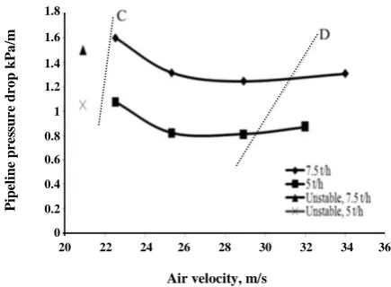
A phase diagram, also referred to as Pneumatic Conveying Characteristics (PCC) diagram [23], is usually a graph of pressure gradient versus superficial air velocity, based on atmospheric conditions, on which lines of constant mass flow rate of solids or solid/air mass flow rate ratio are shown. The PCC diagrams plotted for conveying 4.35 mm diameter wheat particles at two different capacities are shown in Fig. 5. As shown in Fig. 5, by decreasing the air inlet velocity, the pressure drop slightly decreases for the systems working at high air inlet flow rates while increases for those working at lower air inlet flow rates. Studying the pneumatic conveying characteristics of granular materials Wypych & Yi [23] provided a typical Pneumatic Conveying Characteristics (PCC) diagram for granular materials shown in Fig. 6 which consists of three boundaries A, B, and C and the curved boundary D delineating the condition when particles begin to deposit over the bottom of the pipe line.

Comparing Fig. 6 with CFD predicted data on Fig. 5, if the selected air mass flow rate is higher than that for

Fig. 6: Typical PCC for granular materials (Wypych & Yi, 2003).

boundary D, the two-phase flow will be in the form of suspended particles and shows greater energy loss per unit weight of particles by increasing the air flow rate. However, when the conveying air velocity decrease to such extent that is not able to suspend the particles, the flow mode changes to the dense phase region where the conveying is in the form of a suspended layer over a moving bed of deposited particles at the bottom of the tube. In this region, a further decrease in conveying air velocity leads to more deposition and migration of particles from the suspended layer to the moving bed layer at the bottom and therefore the thickness of the moving bed layer increases; thus, the area available for flow of gas is restricted by settled solids. Moreover, low momentum solid particles jump up from the bed and decrease the fluid momentum causing extra increase in pressure drop. According to the boundaries defined by Wypych & Yi [23] the CFD predictions are placed between boundaries C and D on Fig. 6.

However, As depicted in Fig. 4, Guner's measurements show that, the pressure drop over the whole system increases with the air velocity at the inlet boundary, which is characteristic of dilute phase conveying, i.e., beyond the boundary D. To investigate the CFD simulation’s behavior against further increase in air inlet velocity, the simulation was performed for two additional conditions; conveying capacity 7.5 t/h and conveying air velocity 34 m/s, conveying capacity 5 t/h and conveying air velocity 32 m/s. It was observed that the further increase in the conveying air inlet velocity enables it to suspend the granular materials so that now, the conditions locate in dilute phase flow zone. Although

1.8

1.6

1.4

1.2

1

0.8

0.6

0.4

0.2

0

20 22 24 26 28 30 32 34 36

Air velocity, m/s

Pi

p

el

in

e

p

re

ssu

re

d

ro

p

k

P

a

/m

Air mass flow rate

Pr

essu

re

d

ro

Fig. 7: Pressure drop fluctuations against time for conveying air velocity= 28.92 m/s, conveying capacity= 7.5 t/h.

Fig. 8: Model predicted particles volume fraction in the symmetry plane crossed the conveying pipe axis. Conveying air velocity= 22.5 m/s, conveying capacity= 7.5 t/h for (a) the first meter of the conveying pipeline (b) the first 60 cm of the conveying pipeline.

the CFD simulation under-predicted the dilute phase conveying Guner's measurements, the simulation predicted trend shows a very good consistency with other investigators works on dense phase conveying [2,4,11,22-24]. Wypych & Yi [23] observed that the transition from suspension to non-suspension flow is sudden. This sudden change of flow mode is associated with sudden deposition of granular materials as the conveying air velocity decreases and provides an unstable zone in which prediction of the changes of pressure drop with the conveying air velocity is not actually possible. As it is shown on Fig. 5, the simulation predicted data for both loadings includes an unstable point which is shown by a different marker. These two points are located

in the unstable transition zone which is related to the sudden change of flow pattern in pneumatic conveying of granular materials.

Fluctuations in pneumatic conveying system

Pressure fluctuations in the conveying of solids are useful for flow pattern identification [25]. For a specified conveying air inlet velocity, the reduction in available pipe cross-section due to deposition of particles at the bottom, causes an increase in air velocity so that it would be able to suspend more particles and the thickness of deposited materials (i.e., plug) decreases along the pipe. The decrease in plug thickness leads to air velocity (i.e., momentum) decrease and again particles begin to deposit to make the next rolling dune or plug. The formation and deformation of plugs cause sustained fluctuations in pressure drop over the whole pipeline with time for a specified system with constant air inlet velocity. Levy [1] studied pressure variations at specific cross sectional planes along a horizontal tube and depicted the fluctuations due to plug creations and destruction. To see the fluctuations in pressure drop as a typical property of plug flow, pressure drop along the whole pipeline vs. time is depicted for a specific case in Fig. 7. The fluctuations have an average period of about 7 seconds, i.e., 0.14 Hz for system in which the conveying air velocity is 28.92 m/s and the loading is 7.5 t/h which is decreased to 1.5 seconds as the air inlet velocity decreases to 22.5 m/s (not shown) for the same amount of loading. Lee et al [25] also showed the decrease of fluctuations period as a result of a decrease in conveying air inlet velocity experimentally.

CFD model results for the horizontal conveying section Fig. 8 shows the particles volume fraction contour for the first one meter of the pipeline on the vertical plane, passing through the pipe axis, dividing the pipe into two symmetrical sections. As it is shown by Fig. 8, gravitational forces cause the settling of the particles at the bottom of the pipe so that the pipe sectional area can be divided into two layers moving side by side; the upper layer includes suspended particles while the layer at the bottom is the moving bed of settled particles.

As mentioned previously, for a specified air inlet velocity, a portion of pipe cross-section is occupied by the deposited particles (i.e., the plug) which cause

28500

28400

28300

28200

28100

28000

27900

27800

10 15 20 25 30

Time, s

Pr

essu

re

,

d

ro

p

,

P

a

Fig. 9: Model predicted particles volume fraction at y/D=0.05 at different distances from the air inlet boundary. Conveying air velocity= 22.5 m/s, conveying capacity= 7.5 t/h.

an increase in conveying air velocity as it passes over the plug and enables the conveying air to suspend more particles. Since the conveying air suspends the particles, it loses momentum which leads to reduction of its velocity. Reduction of air velocity along the pipe continues so that some particles deposit again and form the next plug. Therefore, as shown in Fig. 8, the thickness of the plug decreases gradually to the point that the next plug forms. Such behavior provides a wave-like form of creation and destruction of plugs which could be easily seen in Fig. 9. In Fig. 9, the particles volume fraction is plotted along the line located at y/D= 0.05 passing throughout the pipeline, which shows that the volume fraction on a specific line in close proximity to the bottom of the pipe (y/D= 0.05) intermittently decrease and increase due to formation and destruction of the plugs. When the particles volume fraction increases to about 0.9 at y/D=0.05, it means that the moving bed depth bordered y=0.05D. In spite, the decrease in the particles volume fraction to about 0.6, shows that the y/D=0.05 line is located in the suspended layer, which means that the wave is dropped off. As shown in Fig. 8, the particle volume fraction decreases suddenly at distances about 2.2, 6.2, and 9.2 m from the air inlet and this shows three successive thin plugs of moving solids (Fig. 9).

Since solid particles settle down at the bottom of the pipe - resulting in a reduction of the pipe available cross sectional area, - air velocity increases and more particles become suspended in the air which leads to gradual

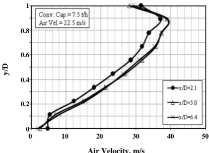
Fig. 10: Normalized air velocity from CFD simulations, at distances x=2.1, 5.0, 6.4 diameter from the point at which the particles introduced to the pipeline. Conveying capacity=7.5t/h and air velocity at the air inlet plane = 22.5 m/s.

decrease of plugs thickness. Levy [1] reported that the slope at the back of the plug wave is steeper than the front and CFD model contour shows this in Fig. 8. Air velocity profiles, plotted along the vertical diameter of the pipe at distances 2.1, 5.0, and 6.4 diameter from the point at which the particles introduced to the pipeline, are depicted in Fig. 10. As it is clearly shown in Fig. 10, one can divide the velocity profile into two parts (e.g., plotting velocity profile at x/D= 2.1, division point can be located at y/D=0.1for conveying of 7.5 t/h of the wheat particles with the air entering at 22.5 m/s), the upper part is associated to the suspended upper layer while the profile at the bottom is associated to the thin moving bed at the bottom of the conveying pipe. Again, as depicted in Fig. 10, stepping forward along the pipe (i.e., increasing x/D), the thickness of the plug decreases gradually till the next plug raised. Therefore, the division point located nearer to the bottom of the pipe or even disappeared if the dunes are discrete from each other.

Fig. 10 also shows that the maximum velocity occurs closer to the top of the pipe which is attributed to the loss of gas-phase momentum because of the higher particle volume fraction near the bottom of the pipe than the top [13,25,26]. Fully developed air flow is arisen when the velocity profiles at different distances from the pipe inlet are the same [25]. Carpinlioglu & Gondugdu [27] studied the development length of two-phase flow using wheat particles with mean diameter of 825 μm and reported that particle shape and size as well as Re have

1

0.8

0.6

0.4

0.2

0

0 1 2 3 4 5 6 7 8 9 10

Z, m

Pr

essu

re

,

d

ro

p

,

P

a

0 10 20 30 40 50

Air Velocity, m/s 1

0.8

0.6

0.4

0.2

0

y

Fig. 11: Normalized air velocity from CFD simulations,

at distances x=2.1, 5.0, 6.4 diameter from the point at which the particles introduced to the pipeline. Conveying capacity=5 t/h and air velocity at the air inlet plane = 22.5 m/s.

great influences on the development length. They reported that the development length decreases as Re increases; and also; the effect of loading ratio on the development length seems to be negligible. Carpinlioglu and Gondugdu observed that fully developed flow for Re=109,000 occurred at 30 < x/D < 40, while for Re > 120,000, the measured fully developed flow to occur at x/D < 10. With reference to the Lee et al [25] criterion for the fully developed flow, i.e., identical velocity profile at different distances from pipe inlet, velocity profiles generated by CFD model was plotted for x/D= 2.1, 5.0, and 6.4 in Fig. 10.

As Fig. 10 shows, the conveying air velocity profiles are identical for x/D > 5; hence, the model predicted the conveying of 7.5 t/h of wheat particles using conveying

air with entrance velocity of 22.5 m/s (i.e., Re140,000) to be fully developed at x/D=5, which is consistent with the Carpinlioglu and Gondugdu results [27]. The model predicted fully development length is also qualitatively consistent with the experimental results provided by Lee et al. [25]. It was also noted by Carpinlioglu and Gondugdu that the loading ratio itself seems not to have much influence on the extent of development length. To study the effect of loading ratio on the extent of fully development length, the velocity profiles were plotted for two different loading ratios, i.e., 5 t/h and 7.5 t/h, while the conveying air velocity at the pipe inlet was the same (i.e., 22.5 m/s). Fig. 11 depicts the velocity profiles for the conveying capacity of 5 t/h. Comparing with Fig. 12

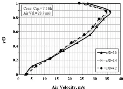
Fig. 12: Normalized air velocity from CFD simulations, at distances x=5.0, 6.4, 9.2 diameter from the point at which

the particles introduced to the pipeline. Conveying capacity= 7.5 t/h

and air velocity at the air inlet plane = 20.9 m/s.

which was plotted for 7.5 t/h of conveying capacity, one can see that fully developed flow again occurred at x/D=5. Therefore, as it was mentioned by Carpinlioglu and Gondugdu, the conveying capacity does not have any significant effect on the development length. To study the effect of Re on the development length and its consistency with Carpinlioglu and Gondugdu's results, air velocity profiles were plotted at distances x/D=5.0, 6.4, and 9.2 (measured from the point at which the particles introduced to the pipeline) for the same conveying capacity as that was plotted in Fig. 12 and with a different air velocity at the air inlet plane that is 20.9 m/s. As Fig. 12 shows, this time fully development occurred at x/D=6.4 which is slightly greater than that of case with air inlet velocity of 22.5 m/s. Hence, as Carpinlioglu & Gondugdu observed, the development length decreases as Re increases.

CFD model results for the flow in the bends Flow in 90° bend

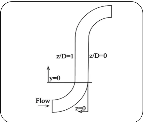
The system simulated in this work includes two 90° elbows; one is horizontal to vertical and the other is vertical to horizontal. A sketch of the elbows is presented in Fig. 13 to show the spatial arrangement of the system.

One of the most important features of gas-solid flow through bends is roping which is attributed to the centrifugal force in the elbow, cause the solid particles to impinge on the outer wall of the bend and forms a relatively dense phase structure referred to as a rope.

0 5 10 15 20 25 30 35 40

Air Velocity, m/s 1

0.8

0.6

0.4

0.2

0

y

/D

1

0.8

0.6

0.4

0.2

0

y

/D

0 5 10 15 20 25 30 35 40

Fig 13: A sketch of the geometry of the end part of the conveying pipe, i.e., where the two elbows are located.

Fig. 14 shows that passing through the elbow, particles are conveyed within a rope in a small portion of the pipe cross-section close to the outer wall due to centrifugal forces (Fig. 14 b). Moving downstream of the elbow in vertical direction, the particles in rope region are accelerated and dispersed in the entire pipe cross-section (Fig. 14 c). Again, due to centrifugal forces in the elbow, most of the particles are conveyed within the rope in a small portion of the pipe cross section close to the top wall of the horizontal pipe at the exit of the elbow (Fig. 14 d). Yilmaz & Levy [16] studied the upward flow in a vertical pneumatic conveying line following a horizontal to vertical elbow and demonstrated that secondary flows spread the particles from within the rope and turbulence creates a more homogeneous distribution of particles. Therefore, turbulence and secondary flows are both responsible for dispersion of the rope.

Akilli [15] studied the characteristics of gas-solid flow in a horizontal pipe following a 90° vertical to horizontal bend and reported that, while moving along the horizontal pipe, the rope dispersed and particles accelerated and spread over the entire cross-section. After dispersion, larger particles travel in the vicinity of the bottom wall of the horizontal pipe as a result of gravity. Therefore, the formation of rope is associated with the migration of particles toward the outer wall of the elbow due to centrifugal forces. As the gas-solid flow exits the elbow the particle rope begin to disperse because of secondary flows and turbulence [16]. To show

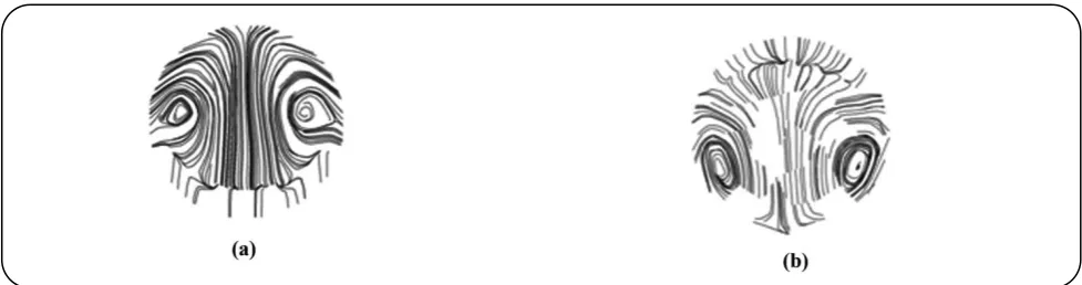
the secondary flows which are responsible for rope dispersions, the air velocity profiles were plotted at each elbow's outlet cross-section (i.e., in the direction of r and θ on cross-sectional planes) in Fig. 15.

Fig. 15a, shows the air velocity profile on a plane located at the horizontal to vertical elbow outlet while Fig. 15b shows them on a plane located at the vertical to horizontal elbow. One can easily see the secondary flows, which carry the particles over the pipe cross section and cause the particles to be spread from the rope, on these two planes; the discontinuities on the lines in these two plans – at the bottom in Fig. 15 b, and the top in Fig. 15a – show the accumulated solid and gas phase interface where the accumulated solid particles and dilute gas phase separates from each other. Secondary flow lines can be seen in the gas phase above the interface in Fig. 15a,

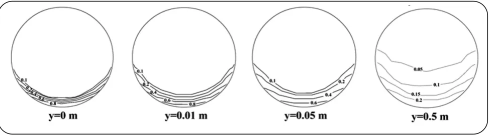
and behind the interface in Fig. 15 b. To provide a better view of rope dispersion, the particles volume fraction contours on the vertical pipe cross sections at different distances from the horizontal to vertical elbow's outlet (i.e., along AA-BB cut in the y direction – see Figs. 13 and 14) are presented in Fig. 16. As depicted in Fig. 16, the rope started to gradually being dispersed as the conveying gas flows along the vertical tube and finally dispersed at distance y/D of about 7 (y = 0.5 m). This observation is consistent with what Yilmaz & Levy [16] reported.

Fig. 14: Predicted solids volume fraction in the symmetry plane of the two 90° elbows at the end of the pipeline, the contour (a) has been cut to three parts (i.e., b, c, d) to provide a magnified view. Conveying capacity= 7.5 t/h,

conveying air velocity= 22.5 m/sec.

Fig. 15: (a) Secondary flow on the horizontal to vertical elbow's outlet cross-sectional plane. (b) Secondary flow on the pipeline outlet boundary, i.e., vertical to horizontal elbow.

of the elbow for different solid conveying capacities at constant conveying air velocity of 22.5 m/s. The particle rope is denser for high conveying capacity and the rate of dispersion is higher for lower values of conveying capacity, which is also consistent with Yilmaz & Levy [16] experimental results.

Fig. 17 shows that the increase in conveying capacity does not affect the rope dispersion; however, it causes the rope to be slightly denser. Similarly, Fig. 18 shows the effect of conveying air velocity on dispersion of the particle rope and particle concentration at different planes of the vertical pipe following the elbow.

Fig 16: Predicted particle volume fraction contour for vertical pipe following the first elbow at different distances, y, from the elbow exit; conveying capacity=7.5 t/h and air velocity=22.5 m/sec.

Fig. 17: Effect of the solids conveying capacity on particle concentration profiles along the pipe diameter in the direction of z at y/D=0, 1, 2, 9, 23.

1.0

0.8

0.6

0.4

0.2

0.0

Pa

rt

ic

le

c

o

n

ce

n

tr

a

ti

o

n

0.0 0.5 1.0

z/D

1.0

0.8

0.6

0.4

0.2

0.0

Pa

rt

ic

le

c

o

n

ce

n

tr

a

ti

o

n

0.0 0.5 1.0

z/D

1.0

0.8

0.6

0.4

0.2

0.0

Pa

rt

ic

le

c

o

n

ce

n

tr

a

ti

o

n

0.0 0.5 1.0

z/D

1.0

0.8

0.6

0.4

0.2

0.0

0.0 0.5 1.0

z/D

Pa

rt

ic

le

c

o

n

ce

n

tr

a

ti

o

n

0.0 0.5 1.0 z/D

1.0

0.8

0.6

0.4

0.2

0.0

Pa

rt

ic

le

c

o

n

ce

n

tr

a

ti

o

Fig. 18: Effect of the conveying air velocity at the air inlet cross-section on particle concentration profiles along the pipe diameter in the direction of z at y/D=0, 1, 2, 9, 23..

velocities, decreasing the conveying air velocity has almost no effect on the dispersion of the rope while it causes the rope to be slightly denser. It worth noting that, as explained in Fig. 16, as flow leaves the horizontal to vertical elbow and passes through the vertical tube, the particle rope gradually disperses in the main stream as y/D increases along the vertical tube.

Flow in U-bend

Fig. 19 shows the effect of horizontal U-bend on the particles volume fraction distribution over the pipe

cross-section at different angles from the U-bend inlet (θ=0°) to the U-bend outlet (θ=180°). As shown, particles migrate near the outer wall due to centrifugal forces and gas accelerates near the inner wall due to the radial pressure gradient; it is also shown in Fig. 20, where the air maximum velocity occurs near the inner wall; In Fig. 20, the conveying air velocity profiles plotted on a horizontal plane passing through the pipe axis.

This is to say that, as shown in Fig. 19, the migration of the solid particles near the outer wall causes the solid particles to collide with the outer wall, so that they

1.0 0.8 0.6 0.4 0.2 0.0 Pa rt ic le c o n ce n tr a ti o n

0.0 0.5 1.0

z/D 1.0 0.8 0.6 0.4 0.2 0.0 Pa rt ic le c o n ce n tr a ti o n

0.0 0.5 1.0

z/D 1.0 0.8 0.6 0.4 0.2 0.0 Pa rt ic le c o n ce n tr a ti o n

0.0 0.5 1.0

z/D 1.0 0.8 0.6 0.4 0.2 0.0 Pa rt ic le c o n ce n tr a ti o n

0.0 0.5 1.0

z/D

0.0 0.5 1.0

Fig. 19: Particles volume fraction contours over the pipeline cross section in the U-bend at different angles. Conveying air velocity= 22.5 m/s, conveying capacity= 7.5 t/h.

Fig. 20: Velocity profiles at different angles within the U-bend. Conveying air velocity= 22.5 m/s, conveying capacity= 7.5 t/h.

decelerate and accumulate on the outer wall of the U-bend in 0° < θ < 60°. The deceleration and accumulation of the particles over the outer wall cause the momentum transfer from gas phase to solid phase to increase; hence, the air velocity near the outer wall is reduced. Consequently, the air maximum velocity is shifted to the outer wall in this region as shown in Fig. 20. For θ > 60°, although the centrifugal effects exist like the previous

region, the gravitational effects move down the particles whose momentum reduced due to the collisions.

Therefore, as shown in Fig. 19, comparing θ=30° and θ=90°, the particles are more concentrated on the outer wall for θ=30°. Therefore, since some of particles moved down at the lower bottom of the pipe in θ > 60°, the effect of the particles integrated on the outer wall on deceleration of the conveying air is less which cause the θ=90° velocity profile in Fig. 20, to have a maximum slightly lower than the maximum in θ=60° velocity profile. For θ > 90°, all of the particles gradually slide down at the bottom of the pipe so that the air velocity near the outer wall in this region is greater than that in the previous regions and consequently the maximum velocity is significantly lower than that in previous regions.

The CFD model predicted results in this region are in a good agreement with what was previously reported by other investigators [12,20]. After the bend, as discussed for 90˚ elbows, particles gradually disperse in the downstream pipe due to turbulence and secondary flow; this is also shown in Fig. 21, as depicted in the particles volume fraction contours, the particles left the outer wall and symmetrically accumulate over the entire bottom part in the absence of centrifugal forces and radial pressure

0 5 10 15 20 25 30 35 40

Air Velocity, m/s 1

0.8

0.6

0.4

0.2

0

y

Fig. 21: Particles volume fraction contours after the U-bend in the downstream pipe. (a) pipe cross-sectional contour immediately after the bend, (b) pipe cross-sectional contour at the distance of 25 cm after the bend, (c) pipe cross-sectional

contour at the distance of 75 cm after the bend.

Fig. 22: Model predicted effect of conveying capacity on the air velocity profile within the U-bend.

gradient. Effect of particles conveying capacity on the air velocity profile depicted in Fig. 22. One can see that the axial velocity for the gas phase increases with the conveying capacity. El-Behery et al. [20] attributed this to the momentum transfer from the solid phase to gas phase because the velocity of solids is greater than that of gas phase in this region. Effect of the inlet air velocity on the air velocity profile is depicted in Fig. 23. As shown the axial velocity in the bend is not highly affected by the gas inlet velocity which is also reported by Hidayat & Rasmuson [12]. Considering the effect of conveying capacity on the pressure drop showed that results predicted by the model concede other investigators’ [20] report on the increase of the pressure drop with the conveying capacity. The increase in pressure drop with particles conveying capacity is observed in the CFD results such that the pressure drop over the U-bend

Fig. 23: Model predicted effect of the inlet air velocity on the air velocity profile within the U-bend.

increases from 6100 Pa to 10000 Pa as conveying capacity increases from 5 to 7.5 t/h at constant air inlet velocity of 22.5 m/s.

Contributions of different piping elements to pressure drop

The prediction of pressure drop along various piping elements is definitely of great importance for design purposes. The pressure drop along different parts of the investigated pneumatic conveyor was studied. It was observed that horizontal pipe, vertical pipe, vertical to horizontal elbow, horizontal to vertical elbow and finally the U-bend are respectively responsible for 65%, 7%, 1.7%, 1.3%, and 25% of the total pressure drop along the whole 23 m long pipeline. Changing conveying capacity and conveying air inlet velocity observed to have almost no effect of the contribution of each element to the total

0 10 20 30 40

Air Velocity, m/s 1

0.8

0.6

0.4

0.2

0

z/

D

0 10 20 30 40

Air Velocity, m/s 1

0.8

0.6

0.4

0.2

0

z/

pressure drop. To reach a reliable index to compare the contribution of elements to the total pressure drop, each of the above ratios is divided by the ratio of the element length to the whole pipeline length. It was revealed that the elements may be arranged from the most to the least effective as U-bend, vertical pipe, vertical to horizontal elbow, horizontal to vertical elbow, and horizontal pipe at last.

CONCLUSIONS

CFD calculations using ANSYS-CFX were performed to investigate the conveying of wheat particles in a pneumatic conveyor with different piping elements. Numerical calculation results validated with the experimental data provided by Guner [10] as well as qualitative trends in literature. In general, the CFD model results for pressure drop are in good agreement with the experimental data. It was observed that better agreements obtained as the conveying capacity increases and dense-phase flow occurs. Constructing conveyer dense-phase diagrams at different operating conditions, the effects of air inlet velocity and the conveying capacity on the flow behavior were also discussed. Both parameters played a significant role in the conveying flow pattern and also the pressure drop. It was shown that CFD model-based phase diagrams could be generated during the system design procedure to assess and predict the optimum operating condition of the pneumatic conveyer. The overall fairly good agreement between the CFD model results and experimental data suggests that CFD can be used productively for investigations and energy consumption optimizations in pneumatic conveying of agricultural and pharmaceutical particles.

Nomenclature

CD Interphase drag coefficient

ds Diameter of solid particle, m

e Solid-solid collision coefficient, energy after collision and before collision g0 Radial distribution function

ug Gas-phase velocity, m/s

us Solid-phase velocity m/s

rg Gas-phase volume fraction

λs Solid bulk viscosity, kg/ms

µg Gas viscosity, kg/ms

µs Solid shear viscosity, kg/ms

ρg Gas-phase density, kg/m3

ρs Solid-phase density, kg/m3

θs Granular temperature, m2/s2

Received : Apr. 3, 2013 ; Accepted : Jun. 22, 2015

REFERENCES

[1] Levy A. Two-Fluid Approach for Plug Flow Simulations in Horizontal Pneumatic Conveying. Powder Technology, 112(3): 263-272 (2000). [2] Konrad K., Dense-Phase Pneumatic Conveying:

A Review. Powder Technology, 49: 1-35 (1986). [3] Mills D., Jones M. G., Agarwal V. K., “Handbook of

Pneumatic Conveying Engineering”, Marcel Dekker (2004).

[4] Pan R., Material Properties and Flow Modes in Pneumatic Conveying. Powder Technology, 104(2): 157-163 (1999).

[5] Rhodes M., “Introduction to Particle Technology”, John Wiley (2008).

[6] Kleinstreuer C., “Two-Phase Flow: Theory and Applications”, Taylor & Francis, (2003).

[7] Snider D. M., O’Rourke P. J., “Gas-Solids Flows and Reacting Systems: Theory, Methods and Practice" (1st ed.), IGI Global (2010).

[8] Sakai M., Koshizuka S., Large-Scale Discrete Element Modeling in Pneumatic Conveying, Chemical Engineering Science, 64(3):533-539 (2008).

[9] Sakai M., Yamada Y., Shigeto Y., Shibata K., Kawasaki V.M., Koshizuka S., Large‐Scale Discrete Element Modeling in a Fluidized Bed, International Journal for Numerical Methods in Fluids, 64(10‐12): 1319-1335 (2010).

[10] Güner M., Pneumatic Conveying Characteristics of Some Agricultural Seeds, Journal of Food Engineering, 80(3): 904-913 (2007).

[11] Pu W., Zhao C., Xiong Y., Liang C., Chen X., Lu P., Fan C., Numerical Simulation on Dense Phase Pneumatic Conveying of Pulverized Coal in Horizontal Pipe at High Pressure, Chemical Engineering Science, 65(8): 2500-2512 (2010). [12] Hidayat M., Rasmuson A., Some Aspects on

Gas-Solid Flow in a U-Bend: Numerical Investigation. Powder Technology, 153(1):1-13 (2005).

[14] Levy A., Mason D. J., The Effect of a Bend on the Particle Cross-Section Concentration and Segregation in Pneumatic Conveying Systems, Powder Technology, 98(2): 95-103 (1998).

[15] Akilli H., Levy E.K., Sahin B., Gas-Solid Flow Behavior in a Horizontal Pipe After a 90° Vertical-To-Horizontal Elbow, Powder Technology, 116(1): 43-52 (2001).

[16] Yilmaz A., Levy E. K., Formation and Dispersion of Ropes in Pneumatic Conveying, Powder Technology, 114(1-3): 168-185 (2001).

[17] Kuan B., Yang W., Schwarz M.P., Dilute Gas-Solid Two-Phase Flows in a Curved 90° Duct Bend: CFD Simulation with Experimental Validation. Chemical Engineering Science, 62(7):2068-2088 (2007). [18] McGlinchey D., Cowell A., Knight E. A., Pugh J. R.,

Mason A., Foster B., Bend Pressure Drop Predictions Using the Euler-Euler Model in Dense Phase Pneumatic Conveying. Particulate Science and Technology, 25(6): 495-506 (2007).

[19] Chu K. W., Yu A.B., Numerical Simulation of Complex Particle-Fluid Flows, Powder Technology, 179(3): 104-114 (2008).

[20] El-Behery S.M., Hamed M.H., El-Kadi M.A., Ibrahim K.A., CFD Prediction of Air-Solid Flow in 180° Curved Duct, Powder Technology, 191(1-2): 130-142 (2009).

[21] Papadikis K., Gu, S., Fivga A., Bridgwater A.V., Numerical Comparison of the Drag Models of Granular Flows Applied to the Fast Pyrolysis of Biomass, Energy Fuels, 24: 2133-2145 (2010). [22] Sanchez L., Vasquez N. A., Klinzing G. E.,

Dhodapkar S., Evaluation of Models and Correlations for Pressure Drop Estimation in Dense Phase Pneumatic Conveying and an Experimental Analysis, Powder Technology, 153(3): 142-147 (2005). [23] Wypych P. W., Yi J., Minimum Transport Boundary

for Horizontal Dense-Phase Pneumatic Conveying of Granular Materials, Powder Technology, 129(1-3): 111-121 (2003).

[24] Mallick S.S., Wypych P.W., Minimum Transport Boundaries for Pneumatic Conveying of Powders. Powder Technology, 194(3):181-186 (2009).

[25] Lee L.Y., Yong Quek T., Deng R., Ray, M.B., Wang C.-H., Pneumatic Transport of Granular Materials Through a 90° Bend, Chemical Engineering Science, 59(21):4637-4651 (2004).