Influence spread in two-layer interdependent networks: designed single-layer or random two-layer initial spreaders?

R E S E A R C H

Open Access

Influence spread in two-layer

interdependent networks: designed

single-layer or random two-layer initial

spreaders?

Hana Khamfroush

, Nathaniel Hudson

, Samuel Iloo

and Mahshid R. Naeini

*Correspondence: [email protected] 1_{Department of Computer Science,} University of Kentucky, University of Kentucky, Lexington 40506, KY, USA Full list of author information is available at the end of the article

Abstract

Influence spread in multi-layer interdependent networks (M-IDN) has been studied in the last few years; however, prior works mostly focused on the spread that is initiated in a single layer of an M-IDN. In real world scenarios, influence spread can happen concurrently among many or all components making up the topology of an M-IDN. This paper investigates the effectiveness of different influence spread strategies in M-IDNs by providing a comprehensive analysis of the time evolution of influence propagation given different initial spreader strategies. For this study we consider a two-layer interdependent network and a general probabilistic threshold influence spread model to evaluate the evolution of influence spread over time. For a given coupling scenario, we tested multiple interdependent topologies, composed of layers AandB, against four cases of initial spreader selection: (1) random initial spreaders inA, (2) random initial spreaders in bothAandB, (3) targeted initial spreaders using degree centrality inA, and (4) targeted initial spreaders using degree centrality in bothAandB. Our results indicate that the effectiveness of influence spread highly depends on network topologies, the way they are coupled, and our knowledge of the network structure — thus an initial spread starting in onlyAcan be as effective as initial spread starting in bothAandBconcurrently. Similarly,random initial spreadin multiple layers of an interdependent system can be more severe than a comparable initial spread in a single layer. Our results can be easily extended to different types of event propagation in multi-layer interdependent networks such as information/misinformation

propagation in online social networks, disease propagation in offline social networks, and failure/attack propagation in cyber-physical systems.

Keywords: Influence spread, Phenomena propagation, Information diffusion, Initial spreader selection, Seed selection, Multi-layer networks, Interdependent networks, Social networks, Cyber-physical systems

Introduction

Multi-layer interdependent networks (M-IDNs) are systems composed of more than one network with edges between them to form an interconnected environment. M-IDNs can be used to model many real-world interdependent systems, such as cyber-physical sys-tems and online-offline social networks. In recent years, we have seen an exponential growth in the development and deployment of these systems. This growth is largely due

to the increasing use of more technologies interfacing with one another — such as the Internet of Things. The explosive expansion and scale of technologies that connect with one another through the Internet provide further incentive to explore the interconnec-tion of different real-world systems and their impacts on phenomena propagainterconnec-tion in these environments.

The interdependency between separate networks creates specific characteristics for these systems that need to be investigated. Specifically, the interaction between separate networks opens up potential for unique opportunities to design new selection strategies that might not be as effective in a system made up of a single network. For example, the attack that was launched by Stuxnet (Albright et al.2010) in 2010 was the result of a malicious computer worm that led to substantial damages to the programmable logic controller (PLC) systems and the power plants. The main reason for such wide-spread damage was the interdependency between the supervisory control and data acquisition (SCADA) system controlling the nuclear enrichment plants and the enrichment plants. This huge impact would likely not have been possible without the interdependency between the cyber (controller) component and the physical component’s performance.

Recently, research aimed at investigating wide-spread phenomena propagation in M-IDNs focuses on designing resilient and robust M-IDN systems. There is a considerable amount of literature addressing the problem of modeling and analyzing the impact of interdependency between different interdependent systems (such as cyber-physical systems) and how to minimize phenomena propagation in these systems. Work inves-tigating selection strategies of initial spreaders in M-IDN systems has been conducted (as discussed in Related Work section). However, these works consider less general propagation models like epidemic and independent cascade. Additionally, our work is particularly interested in investigating how the evolution of affliction over time and a vari-ety of interconnectivity and layer-based selection strategies for initial spreaders compare, distinguishing our work from that in the literature.

In short, we will make the following contributions:

• We propose a modified version of the threshold-based phenomena propagation model that was initially proposed in (Khamfroush et al.2016) for a general interdependent network and a single phenomenon, as a mathematical model to quantify the impact of different strategies for selecting initial spreaders for phenomena propagation in an M-IDN system.

• We perform extensive simulations to study the effectiveness of different types of spread initialization including random/designed single-layer initial spread and random/designed multi-layer initial spread in a M-IDN system.

• We provide guidelines on which network topologies and types of coupling between the networks provide faster propagation when facing different strategies for spread initialization. Due to the generality of the proposed model, our observations provide a useful framework for further investigation and design of robust and reliable M-IDN.

Related work

(Kim et al.2014; 2015; Kandhway and Kuri2017) or minimize the propagation of mis-information (or “fake news”) (Papanastasiou2018; Kimura et al.2009; Shu et al.2019). Since our problem is general in nature, we do not consider a context that implies whether the phenomena propagation has positive or negative ramifications. We are simply inter-ested in how certain selection strategies of initial spreaders affect overall phenomena propagation.

Securing an M-IDN goes beyond securing the separate networks composing the entire interdependent topology. Adversaries are willing to use the interdependency of vul-nerabilities to carry out multi-stage attacks. Each facet of an attack may not pose a significant threat to a single network on its own; however, cumulative influences through interdependency, may have catastrophic effects.

In the past few years, vulnerabilities in M-IDNs have been widely studied. In general, there are two main approaches to study this vulnerability. The first approach typically involves focusing on a certain application of M-IDNs to identify different forms of attacks/threats and potential strategies to protect corresponding M-IDN systems. For example, (Anderson and Fuloria2010; McDaniel and McLaughlin2009; Metke and Ekl 2010; Mo et al. 2012; Rahman et al. 2012) looked into financially motivated threats in smart grids where a customer who wants to trick a utility company’s billing system tam-pers with smart meters to reduce the electricity bill. Other studies, such as (Halperin et al.2008; Hanna et al.2011; Rushanan et al.2014), looked into the threats against medical cyber-physical systems. Authors in (Brooks et al.2008; Checkoway et al.2011; Hoppe et al.2008) defined and investigated different threats in smart cars as another application of cyber-physical systems.

In our prior work (Hudson et al.2019), we investigate the effectiveness of standard and interdependent centrality metrics to minimize cascade of failure. In that work, we used random failure to select initially failed nodes to begin failure propagation. There was no investigation, in this prior work, into how different strategies for initial spread performed.

problem that focuses on choosing optimal seed set such that the spread of information is maximized, e.g., (Michalski et al.2014; Kempe et al.2005; Chen et al.2009; Chen et al. 2010).

In contrast to these prior works, our goal is not to find the most influential seed set, instead we are looking at the impact that different choices of the seed set (single-layer versus two-layer) could have on the propagation process. More specifically, we are inves-tigating whether a single-layer seed selection could be as influential as a similar size two-layer seed selection. Furthermore, our study incorporates a more general propaga-tion model and takes into considerapropaga-tion the evolupropaga-tion of the spread of a phenomenon over time. This consideration allows afflicted nodes more opportunities to afflict neighbor nodes, which is more realistic in many scenarios. For instance, in the context of informa-tion cascade in social networks one user may be afflicted by some informainforma-tion and share that with their friends. This person’s friends may not immediately adopt the information that this person is propagating; however later in time this could change. The independent cascade model does not consider such cases and is thus inapplicable for many scenar-ios that involve delay. Further, linear threshold and linear probabilistic propagation are special use cases of our model.

Problem statement

We consider an M-IDN system consisting of two interdependent networks, A and B. Both layers A and B are represented by two undirected graphs GA = (VA,EA) and

GB=(VB,EB), whereVAandVBrepresent the sets of vertices in layersAandB (respec-tively) andEAandEBrepresent the sets of edges in layersAandB(respectively). It is assumed that|VA| =NAand|VB| =NB. Though it is not contingent forNAto be equal toNB, for our experimentsNA =NBin all synthetic cases. The two networks are inter-connected by means of directed edges. We refer to edges that connect nodes belonging to the same networks as intra-edges and those that connect nodes belonging to differ-ent networks as inter-edges. We use directed edges for inter-edges to capture differdiffer-ent models of inter-dependency between networks. Without loss of generality, it is assumed that an initial set F0 = F0A∪F0B of nodes are afflicted initially, where F0A represents

the set of initial spreaders in networkAandF₀Brepresents the set of initial spreaders in layerB. Phenomena can propagate among nodes belonging to the same network. In addi-tion, phenomena can also propagate across networks, such as phenomena propagating from a node in layerA to a node in layer B(or vice-versa) through inter-edges. Phe-nomena propagation takes place with respect to a threshold-based propagation model — as discussed in more detail in “Phenomena propagation model” section. Given an M-IDN system with a known topology, we are interested in comparing the rate of phe-nomena propagation with respect to time under different types of initial spreads. More specifically, given an initial set of afflicted nodesF0(“initial spreaders”), we will evaluate

phenomena propagation in an M-IDN system. The goal of this work is to provide use-ful guidelines on how to design reliable M-IDN systems. Additionally, we are particularly interested in the evolution of phenomena propagation in the case of single- and two-layer affliction.

• Random single-layer spread is represented by defining|F₀A| = |F0|and|F₀B| =0,

where the nodes ofF₀Aare chosen randomly1.

• Random two-layer spread is represented by defining|F₀A| = |F0|/2and|F0B| = |F0|/2,

where the nodes ofF₀AandF₀Bare chosen randomly.

• Designed single-layer spread is represented by choosing|F0|nodes belonging to layer

A with highest degreeF₀A, and setting|F₀B| =0.

• Designed two-layer spread is represented by choosing|F0|/2nodes belonging to layer

A with highest degreeF₀Aand|F0|/2nodes belonging to layerB with highest degree

F₀B.

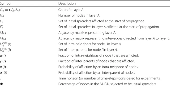
Due to the general nature of our problem, we are not seeking to differentiate negative and positive phenomena propagation. We are simply interested in how certain selection strategies for initial spreaders affect overall phenomena propagation. For this reason, we refer to nodes that have been affected by the phenomena propagation as “afflicted” and the process by which nodes are afflicted as “affliction”. This language is used to avoid the contextual effects of phenomena propagation for different domains. For an overview of the notation defined throughout this paper, refer to Table1.

Phenomena propagation model

Many threshold-based propagation models rely on deterministic behavior; wherein if a proportion of a node’s neighbors are afflicted, then it will be afflicted definitively. While this approach is appropriate for epidemic phenomena, this approach to phenomena prop-agation is not as general and fails to consider cases with probabilistic propprop-agation. Due to this limitation we incorporate a modified version of probabilistic threshold-based phe-nomena propagation used in our prior works (Khamfroush et al.2016; Hudson et al. 2019). As in our prior works, we considered nodes belonging to the same network to have peer roles and thus are connected through undirected edges. We refer to the adjacency matrices that represent layersAandBasMAA ∈ {0, 1}NA×NA andMBB ∈ {0, 1}NB×NB, respectively. The interconnectivity between layersAandBcan be represented as inter-connection adjacency matricesMAB ∈ {0, 1}NA×NB andMBA ∈ {0, 1}NB×NA — with the

Table 1Summary table of noteworthy notation introduced

Symbol Description

GA=(VA,EA) Graph for layerA.

NA Number of nodes in layerA.

F0 Set of initial spreaders afflicted at the start of propagation. F₀A Set of initial spreaders in layerAafflicted at the start of propagation.

MAA Adjacency matrix representing layerA.

MAB Adjacency matrix representing inter-edges directed from layerAto layerB.

Uintra

A (i) Set of intra-neighbors for nodeiin layerA.

Uinter_A (i) Set of inter-parents for nodeiin layerA.

α(i) Fraction of intra-neighbors of nodeithat are afflicted.

β(i) Fraction of inter-parents of nodeithat are afflicted.

π(i₎ Probability of affliction by an intra-neighbor of nodei.

π_{(i) Probability of affliction by an inter-parent of nodei.}

T Time horizon (or number of time-steps) considered for experiments.

former representing directed edges from layerAto layerBand the latter representing the opposite.

We consider two nodes belonging to the same network with edges between each other as intra-neighbors. Additionally, we consider a nodeiwith a directed edge to a nodej that belongs to a different network as an inter-parent. Formally, the set of intra-neighbors for nodei in some layerAcan be defined asU_Aintra(i) = {j ∈ A | (i,j) ∈ EA}, with

|U_Aintra(i)|representing the intra-degree of nodei ∈ A. Further, we formally define the set of inter-parents belonging to some layerBof a nodeibelonging to some layerAas U_Ainter(i)= {j∈B|MBA(j,i)=1}.

Under this model, a node has a probability that it will become afflicted only under the case that the proportion of its afflicted neighbors reach or exceed the designated thresh-old. This model relies on specified a pmax value for each set of connectivity between

networks — for our work, we considerp_max(AA), pmax(AB),pmax(BB), andpmax(BA). This

is a general parametric model that incorporates many previous models as special cases. For the two networks composing the M-IDN topology for our study, we introduce two different threshold functions:kaa(i) ∈ (0, 1] fori ∈ A, andkbb(i) ∈ (0, 1] fori ∈ Bto model the propagation across the nodes of the same network. We also introduce two other threshold functions:kab(i) ∈ (0, 1] fori ∈ B, andkba(i) ∈ (0, 1] fori ∈ A, to model propagation across the two interdependent networks, from layerAto layerBand vice versa, respectively. We denoteπ(i)to be the probability of phenomena propagation to afflict nodeidue to the propagation of intra-neighbors ofi, andπ(i)to be the probability of phenomena propagation to afflict nodeidue to the propagation of inter-parents ofi.

Assuming that a fraction α(i) of intra-neighbors of nodei are already afflicted, the probability that phenomena propagates to nodeiwithin one time-step is defined in Eq.1,

π(i)=

α(i)·pmax(AA)(i) if α(i)≥kaa(i) 0 if α(i) <kaa(i)

(1)

where pmax(AA)(i) represents the probability that node i is afflicted within one time step, when all of its intra-neighbors are already afflicted. Similarly, nodeimay become afflicted due to the propagation of some of its inter-parents. Letβ(i)be the fraction of inter-parents of a nodeithat are already afflicted. Thus, the probability that phenomena propagates from inter-parents of nodeito nodeiwithin one time step is calculated as defined in Eq.2,

π(i)=

β(i)·p_max(AB)(i) if β(i)≥kba(i) 0 if β(i) <kba(i)

(2)

wherepmax(BA)represents the probability that nodeiin layerAis afflicted within one time step, when all of its inter-parents inBare already afflicted. We use a similar notation for nodej∈ Bby defining equations analogous to Eqs.1and (2), where we use the thresh-oldskBB andkAB to express the required fraction of intra-neighbors and inter-parents of node j that must be afflicted beforejcan become afflicted with positive probability. Also, the probability that nodejin layerBis afflicted within one time step, when all of its inter-parents inAare already afflicted will be shown bypmax(AB). Note thatpmax(AB)and

Generalization for many layers

This model can easily be extended to consider M-IDN topologies consisting of some abstractmlayers. In this work, we only consider M-IDN topologies with two layers, so we provide notation to understand the formal definitions of this model with respect to that (e.g.,MAA, pmax(AB), etc.). However, this model can also be used to consider M-IDN topologies made of more than two layers. For instance, in an M-M-IDN topology of three layers (A,B, andC), you would consider all the same formal definitions, but include parameter permutations that involveC— such asMCC,MCA,MAC,MCB,MBC, etc.

The decision to solely focus on M-IDN topologies of two layers for this work was moti-vated by the curiosity to explore how varying interconnectivity, selection strategies, sizes, and other parameters affect the evolution over time of the phenomena propagation pro-cess. More specifically, we would like to study to what extent interdependency between networks and the knowledge of network topology can help the speed of propagation in a M-IDN network.

Phenomena propagation process

The temporal evolution of phenomena propagation is modeled as a Markov model. This is because the next state of the network will only depend on the current state of the network and it is independent of how the network reaches its current state. In the following, we describe the elements of our proposed Markov model.

State definition

We denote bySTthe set of all possible states of the model, where each state is defined as

a vectors = (

A

s1,s2,. . .,sNA,

B

sNA+1,sNA+2,. . .,sNA+NB), wheresi = 1 fori ≤ NAif node i ∈ Ais afflicted, andsi = 0 if it is not afflicted. Similarly, fori > NA,si = 1 is one if nodei−NAof layerBis afflicted, andsi =0 otherwise. Therefore, the initial state of the phenomena propagation process isS0=(s1,s2,. . .,sNA,sNA+1,sNA+2,. . .,sNA+NB), where sk =1 ifk≤NA∧k∈A∩F0Aork>NA∧k∈B∩F0B, whilesk =0 otherwise.F0Aand

F₀Bare the set of initial spreaders in layersAandB, respectively.

According to our proposed model, a node can become afflicted only if the proportion of its afflicted intra-neighbors and/or inter-parents exceed a given threshold. Therefore, not all the binary vectors ofNA+NBelements represent a feasible state of the process. Note that a node of layerAmay become afflicted due to the consequences of the initial spreaders in layerA, layerB, or both. The goal of this paper is to analyze the impact of concurrent phenomena propagation in M-IDNs to gain a better understanding of the most robust interdependent network topology. Our propagation model and the Markov model provide a general framework that allows for further investigation of different types of phenomena propagation/impact.

Transition probabilities

Based on our previous definitions, we calculate the one-step transition probability matrix of the process℘ ∈ {0, 1}|ST|×|ST|_{, whose generic element}℘|

s,s gives the probability that the network transits from statesto states. We lets=s−s. Thej-th element of vectors

sj = 1. We denote an indicator functionI(cond)where condis a boolean value and

I(true)=1,I(false)=0. A formal definition for℘|s,s is provided in Eq.3,

℘|s,s = NA+NB

j=1

f(j)I(sj=0)+f(j)I(sj=1) , (3)

wheref(j)denotes the probability that there is no change in thej-th component of the network state when transitioning from statesto states, andf(j)is the probability that there is a change of status for thej-th node of the network, going from a working node to a afflicted node. It is important to note thatsj =0 happens in two cases:i) the related node is already afflicted, as we do not consider recovery or restoration of the network in this paper, andii) the related node is currently working and it will remain the same as the proportion of afflicted neighbors/parents does not meet the threshold or, although the propagation threshold is met, the propagation did not occur in the current time-step (referring to the probabilistic nature of the propagation model).

We also calculate the value off(j)andf(j)by separating the terms related to layersA andB. In particular, the probability of having a change in thej-th element of the inter-dependent network when the network state changes fromstoscan be calculated in the definition for Eq.4.

f(j)=

⎧ ⎪ ⎨ ⎪ ⎩

ga(j) if j≤NA∧sj=0

gb(j) if j>NA∧sj=0 1 if sj=1

(4)

Then,ga(j)can be calculated as defined in Eq.5,

ga(j)=I(α(j) <kaa(j))·I(β(j) <kba(j))+

I(α(j)≥kaa(j))·I(β(j) <kba(j))· ¯π(j)+

I(α(j) <kaa(j))·I(β(j)≥kba(j))· ¯π(j)+

I(α(j)≥kaa(j))·I(β(j)≥kba(j))· ¯π(j)· ¯π(j)

(5)

whereπ(¯ j)=1−π(j)andπ¯(j)=1−π(j), withπ(j)andπ(j)defined in Eqs.1and2, respectively.

The termgb(j), will be similarly calculated for the nodes located in layerB, by replacing

kaawithkbb, andkbawithkabin Eq.5. Note that according to our definition, the nodes of the M-IDN system are enumerated from 1 toNA+NB, therefore,kaaandkbaare only defined forj≤NAandkbb,kabare only defined forNA<j≤NA+NB.

The termf(j)denotes the probability that there is a change in thej-th component of the state vector, when the network is transitioning from statesto states. We splitf(j)in the contributions related to the two layersAandB. Therefore,

f(j)=

⎧ ⎪ ⎨ ⎪ ⎩

g_a(j) if j≤NA∧sj=0

g_b(j) if j>NA∧sj=0 0 if sj=1

(6)

Similar to our previous note, we can calculate the termg_a(j)as follows, g_a(j)=I(α(j)≥kaa(j))·I(β(j)≥kba(j))·

π(j)π(j)+ ¯π(j)π(j)+π(j)π¯(j)

+

I(α(j) <kaa(j))·I(β(j)≥kba(j))·π(j)+

I(α(j)≥kaa(j))·I(β(j) <kba(j))·π(j)

Using a similar argument, we can write similar equations for the nodes in layerB, i.e.g_b(j) can be calculated.

Note: Based on the definition of transition probabilities, we observe that the speed of phenomena propagation will increase, if and only iff(j) f(j)in Eq.3. This is because, under this condition, the second term in Eq.3 will dominate the transition probabil-ity, meaning that the probability that sj = 1 is much larger than that of sj = 0, therefore the number of afflicted nodes increases faster over time. Looking atf(j)and f(j), we can see that both are functions ofpmax(∗∗). By increasing the value ofpmax(∗∗), we will have f(j) > f(j), asf(j) is an increasing function of π and π, and thus an increasing function ofpmax(∗∗). On the other hand,f(j)is a decreasing function of these probabilities.

Expected absorption time

Phenomena propagation in an M-IDN system can be seen as an absorbing Markov chain, where the absorbing states are defined as one of the following:i) all nodes of the M-IDN system are afflicted, andii) no working node can meet the phenomena propagation con-dition. The set of absorbing states depends on the sets of initial spreadersF₀AandF₀B and the propagation thresholds. Therefore, we may get different absorbing states for the same network topology when the set of initial spreaders inAandBare different. Given that we have the states of the network and transition probabilities, we can use standard techniques, used in (Charles et al.1997), for analyzing our proposed Markov process and to calculate the expected absorption time. However, the state space for a reason-ably sized network would be very large as we are considering the state of a network’s individual elements. Due to this limitation, we have only tested our model using net-works of a relatively small size for the proposed Markov model. We then use this to validate the correctness of our simulations that have been built to handle networks of larger sizes while using the same phenomena propagation model. An example of sim-ulation validation can be found in (Khamfroush et al.2016). As the focus of this work is to use extensive simulations to provide useful guidelines on the vulnerability of dif-ferent network topologies, we focus on simulation setup and results in the following sections.

Description of experiments

We investigate how different initial spreader selection strategies affect phenomena prop-agation in M-IDN systems. To study this, we perform and analyze extensive simulations. To be thorough, we consider the time evolution of phenomena propagation of M-IDN systems with varying network topologies, coupling strategies, inter-edge density, average degree, and the choice of initial spreaders. For this work, we are particularly interested in how single-layer initial spread in Scenarios 1-1 and 2-1 compares to multi-layer initial spread in Scenarios 1-2 and 2-2.

Tested scenarios

“single-layer selection” or “two-“single-layer selection”. If a scenario uses the former, then “single-layerAwill have|F0| nodes selected as initial spreaders; if a scenario uses the latter, then layersA

andBwill both have|F0|/2 nodes selected as initial spreaders. Below are the scenarios

considered:

• Scenario 1-1:Single-layer selection, initial spreaders chosen at random.

• Scenario 1-2:Two-layer selection, initial spreaders chosen at random.

• Scenario 2-1:Single-layer selection, initial spreaders chosen by high degree centrality.

• Scenario 2-2:Two-layer selection, initial spreaders chosen by high degree centrality.

Interconnectivity models

For our simulations, we consider a variety of interconnectivity for thorough examination of our core question. With this in mind, we consider the notion of inter-connections (rep-resented by directed inter-edges) being established atrandomor bydesign. Additionally, we also aim to explore howloworhighnumbers of inter-connections affect phenomena propagation.

There are a lot of considerations in our interconnectivity model. First, we introduce the four interconnectivity cases considered in our experiments:

• Sparse & Random:In this model, 8% of nodes are selected to have inter-edges directed to nodes in the other network. 4% of nodes in layerA (chosen at random) have inter-edges to nodes in layerB (chosen at random), and vice versa.

• Dense & Random:In this model, 20% of nodes are selected to have inter-edges directed to nodes in the other network. 10% of nodes in layerA (chosen at random) have inter-edges to nodes in layerB (chosen at random), and vice versa.

• Sparse & Designed:In this model, 8% of nodes are selected to have inter-edges directed to nodes in the other network. 4% of nodes in layerA (based on degree centrality) have inter-edges to nodes in layerB (based on degree centrality), and vice versa.

• Dense & Designed:In this model, 20% of nodes are selected to have inter-edges directed to nodes in the other network. 10% of nodes in layerA (based on degree centrality) have inter-edges to nodes in layerB (based on degree centrality), and vice versa.

Additionally, in the case of designed interconnectivity (Sparse-Designed or Dense-Designed), we consider how nodes are chosen to have inter-edges. We are interested in exploring how nodes of high degree and low degree affect the evolution of phenomena propagation. For this, we consider three cases of how designed selection of nodes with inter-edges takes place:

• Max-Max:Nodes of highest degree in the currently considered network are designed to have inter-edges to nodes of the highest degree in the other network, and vice versa.

• Max-Min:Nodes of highest degree in layerA are designed to have inter-edges to nodes of the lowest degree in layerB and nodes of lowest degree in layer B have inter-edges to nodes of highest degree in layerA.

Tested network topologies Synthetic topologies

For synthetic topologies, we use three well-studied random generative models for net-work topologies: Erdös-Rényi (ER) model (Erdos and Rényi1960), Barabási-Albert (BA) model (Barabási and Albert1999), and the Watts-Strogatz (WS) model (Watts and Stro-gatz1998). The ER model produces what are commonly referred to as purely random graphs; the BA model produces topologies that maintain a power law degree distribution; and the WS model produces topologies with the small-world property.

To be thorough, we consider all permutations of the random generative models for a two-layer M-IDN topology. For instance, an M-IDN topology composed of two layersA andBthat are both constructed by the ER model will be referred to as an ER-ER topology (coinciding withA-B). It is important to note that network topologies are not transitive in our experiments — i.e., an ER-SW topology is not equivalent to an SW-ER topology. The reason for this is that a single-layer selection scenario only selects initial spreaders in layerA, thus a simulation using an ER-SW topology is not comparable to a simulation using an SW-ER topology. To be clear, in all of our experiments, we generate a synthetic, random M-IDN topology in each Monte-Carlo run.

Real-world topologies

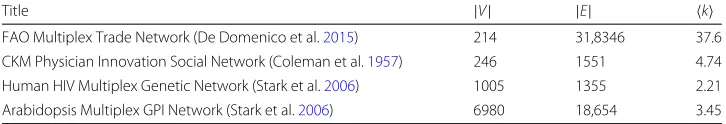
For comparison, we also run simulations using real-world multiplex topologies. These topologies come from different domains — social networks, genetic networks, etc. A key difference between these topologies and our synthetic topologies is the inter-connection between layers A and B. In our synthetic topologies, we consider Sparse/Dense and Designed/Random inter-connections. In our real-world topologies, each node exists across all layers with inter-edges to each other node corresponding to it across all layers. For a concise description o fhte real-world topologies considered for this work, refer to Table2.

Simulation setup

Here, we review some of the constants that are maintained across all simulations consid-ered for our experiments and review some other experimental choices that have not been addressed thus far. For any simulation setup, we consider the evolution of phenomena propagation over a time horizon ofT = 200 time steps. In the plots presented for our results, we let the x-axis represent the time steps comprising the time horizonT; while the y-axis represents the number (or percentage) of afflicted nodes in the entire M-IDN topology.

Table 2Overview of the real-world multiplex network topologies considered for simulations in this work

Title |V| |E| k

FAO Multiplex Trade Network (De Domenico et al.2015) 214 31,8346 37.6

CKM Physician Innovation Social Network (Coleman et al.1957) 246 1551 4.74

Human HIV Multiplex Genetic Network (Stark et al.2006) 1005 1355 2.21

Arabidopsis Multiplex GPI Network (Stark et al.2006) 6980 18,654 3.45

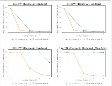
Additionally, for our synthetic networks, we consider cases whereNA = NB = 100 and NA = NB = 500. For all synthetic topologies, we consider an average degree

k =4. We evaluated how average degree affects phenomena propagation before mak-ing this decision. For our considered threshold parameter values, we observe that higher average degree corresponds with significantly less affliction throughout the phenomena propagation process — refer to Fig.1.

Additionally, we are interested in the cases where values for our probabilistic threshold-based model are i) the same for layer Aand B andii) where they are different. The former case is what we refer to as homogeneous propagation while the latter case is referred to as heterogeneous propagation. For heterogeneous propagation, we use the following threshold values:kaa = 0.5,kbb = 0.2,kab = 0.3, andkba = 0.8. For homo-geneous propagation, we use the following threshold values: kaa = kbb = 0.3 and

kab= kba= 0.5. These threshold values are used for all simulations, both synthetic and real-world.

Results

To reiterate, we consider a variety of parameters for a simulation. To cope for random-ness, each simulation setup is run a number ofM=100 Monte Carlo runs, with results being averaged across these runs. Due to the sheer number of parameters considered, our results span hundreds of simulation setups. Therefore, we want to highlight important pieces of data analysis in hopes that key conclusions can be made. So, we elect to show plots of some of the more interesting simulation results and will describe general trends

throughout. For brevity, we say “single-layer selection” to refer to Scenarios 1-1 and 2-1 and “two-layer selection” to refer to Scenarios 1-2 and 2-2.

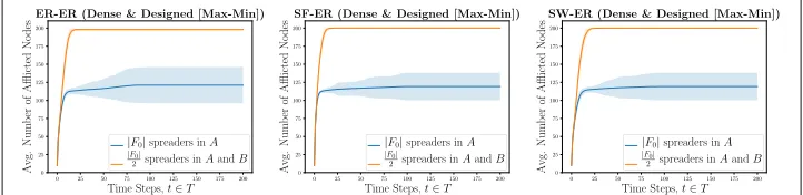
Interestingly, for the interconnectivity cases we consider for this work, a noteworthy trend across most synthetic simulation setups is that two-layer selection of initial spread-ers appears generally to be more effective than single-layer selection in affecting the entire M-IDN topology. In many cases, this selection strategy afflicts the entire M-IDN topology early in the propagation process; whereas the propagation under single-layer selection commonly saturates early in the propagation process without afflicting the entire topol-ogy (or full affliction is attained after two-layer selection). As an additional observation, we observed that as we experimentally increased average degreek, single-layer selec-tion outperforms two-layer selecselec-tion — this was observed before designatingk =4 but we felt worth mentioning. We also note that asincreases, generally two-layer selection outperforms single-layer seleciton.

Homogeneous simulations

Here we investigate the results of our homogeneous simulations. As a reminder, we refer to homogeneous simulations as simulations where the threshold values for our prop-agation model are constant across both layers A and B in the layers of our M-IDN topology.

Intuitively, Sparse interconnectivity essentially dampens the possible effects of phenom-ena propagation under our model. Our results reflect this intuition. Refer to Fig.2for a sample of these simulation results. For a detailed overview of affliction w.r.t. to time evolution, refer to Table3. Overall, we see in the homogeneous case, that Scenario 2-2 (two-layer selection by degree centrality) is the most effective (w.r.t. to time and per-centage of affliction) at reaching near full affliction across most interconnectivity cases considered.

Designed max-max

We observe for homogeneous simulations with Dense interconnectivity that the variance across Monte-Carlo runs isincredibly small across all considered topologies, network sizes, and. This observation makes sense upon further consideration. Consider the BA random model for network topologies. Due to preferential attachment, nodes are more likely to coalesce and associate with nodes of high degree (forming “hubs”) — which are selected to exhibit interconnection under Scenarios 2-1 and 2-2. If the central, highly

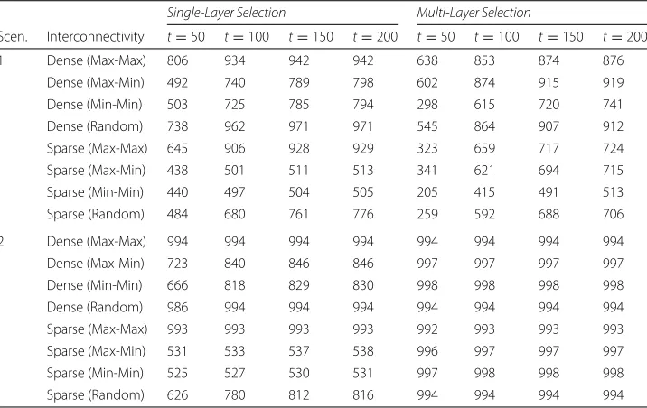
Table 3Homogeneous data for whenNA=NB=500 and=3%

Single-Layer Selection Multi-Layer Selection

Scen. Interconnectivity t₌50 t₌100 t₌150 t₌200 t₌50 t₌100 t₌150 t₌200

1 Dense (Max-Max) 806 934 942 942 638 853 874 876

Dense (Max-Min) 492 740 789 798 602 874 915 919

Dense (Min-Min) 503 725 785 794 298 615 720 741

Dense (Random) 738 962 971 971 545 864 907 912

Sparse (Max-Max) 645 906 928 929 323 659 717 724

Sparse (Max-Min) 438 501 511 513 341 621 694 715

Sparse (Min-Min) 440 497 504 505 205 415 491 513

Sparse (Random) 484 680 761 776 259 592 688 706

2 Dense (Max-Max) 994 994 994 994 994 994 994 994

Dense (Max-Min) 723 840 846 846 997 997 997 997

Dense (Min-Min) 666 818 829 830 998 998 998 998

Dense (Random) 986 994 994 994 994 994 994 994

Sparse (Max-Max) 993 993 993 993 992 993 993 993

Sparse (Max-Min) 531 533 537 538 996 997 997 997

Sparse (Min-Min) 525 527 530 531 997 998 998 998

Sparse (Random) 626 780 812 816 994 994 994 994

Each value corresponds to the average number of afflicted nodes at the respective time-step,t, across all considered Monte-Carlo runs for all synthetic topologies

connected node of this hub is afflicted, its lesser connected neighbors are more vulner-able to affliction because that high degree node likely makes up a sizvulner-able proportion of its neighbors (thus having more impact on its threshold to affliction). For homogeneous simulations with Sparse interconnectivity, we also see very little variance — though not as small.

For Dense interconnections, generally the single-layer selection of initial spreaders out-performs the two-layer selection strategy. The difference between these two strategies in this setup is not particularly notable, but the general trend is that single-layer selec-tion is slightly more effective. Meanwhile, for Sparse interconnecselec-tions, the general trend holds. However, the difference between single-layer and two-layer selection strategy is more prominent. Additionally, it is important to note that asincreases, the two-layer selection strategy begins to outperform the single-layer selection strategy. This implies that if you have more budget to select more initial spreaders under these parameters, two-layer selection would be most effective. However, if you have a more conservative budget, single-layer selection would be more appropriate.

Designed max-min

For both Dense and Sparse interconnectivity, we observe that our averaged data shows that two-layer selection notably outperforms single-layer selection in allcases. Under Dense interconnectivity, the variance of the resulting phenomena propagation for single-layer selection is notably large; while the variance of the resulting phenomena propagation for two-layer selection in this case is very small. However, under Sparse interconnec-tivity, the variance of the resulting phenomena propagation for single-layer selection is significantly smaller than under Dense interconnectivity.

simulation using single-layer selection having comparable affliction rates to two-layer selection. The performance of single-layer selection is starkly less impressive under Sparse interconnectivity — with propagation saturating early on with about 50% affliction across all cases. This is likely due to initial spreaders exclusively selected in layerApropagate affliction to nodes minimum degree nodes in layerB. As a result, layerAis roughly 90% afflicted whereas layerBroughly 10% afflicted.

Designed min-min

With an increase in the size of the networks, single-layer selection is notably more effec-tive than in smaller network sizes — reaching full affliction (on average) in some cases. Otherwise, results for this set of experiments is very comparable to Designed Max-Min. However, there does appear to be less variance for single-layer selection. In the Max-Min case, some nodes in the layer Bcan cross-propagates though maximum degree nodes under two-layer selection. However, in the case of Min-Min, it this does not happen. This is likely why the difference is not as initially prominent.

Random

There is a stark difference between Dense interconnectivity and Sparse interconnectivity in this case. In Dense interconnectivity, the performance between single-layer selection and two-layer selection is marginal — though two-layer selection has a slight edge. Both selection strategies, on average, result in full affliction (or very close to it) in all cases considered — whenNA=NB=500 all experiments reached full affliction. Additionally, variance of performance was very low under Dense interconnectivity. It should be noted that whenis a low value (e.g.,=3%), there is a split in certain topologies where single-layer selection performs better in terms of overall affliction. However, asincreases, two-layer selection begins to close the gap in these topologies and eventually overtakes it in terms of affliction w.r.t. to time.

These remarks cannot be made for this experiment under Sparse interconnectivity. WhenNA= NB =100, the performance of single-layer selection would typically hover in the range of about 50%-70% affliction.

Heterogeneous simulations

Here we investigate the results of our heterogeneous simulations. As a reminder, we refer to heterogeneous simulations as simulations where the threshold values for our propaga-tion model are unique across both layersAandBin the layers of our M-IDN topology. There are no standout trends across the different models of interconnectivity. Below is a brief summary of the general behavior of these simulations. Generally, for the Het-erogeneous case (under the threshold values we use), the most apparent trend is that single-layer selection seems to be a more potent selection strategy overall than two-layer selection. It is important to note that this trend is not guaranteed to hold for different threshold values under this propagation model.

due to its robustness since half of the resources for selection are used on the vulner-able layer. For a more detailed overview of affliction w.r.t. to time evolution, refer to Table4.

For both Sparse and Dense interconnectivity, whenNA=NB=100, the general trend is that two-layer selection outperforms single-layer selection when the percentage of nodes selected to be initial spreaders is smaller. Once 10% of the nodes are selected to be initial spreaders, for both cases, the single-layer selection strategy begins to overtake the two-layer selection strategy. However, the difference in performance is marginal and not highly significant.

However, whenNA=NB=500, under Dense interconnectivity, the strategies perform nearly identically until 10% of nodes are selected as initial spreaders. In which case, single-layer selection begins to have the advantage. The advantage in this case, is notable and is quite significant when compared to the experiments whereNA = NB = 100. Also, the variance in the resulting phenomena propagation is very high when the percentage of nodes selected to be initial spreaders is small.

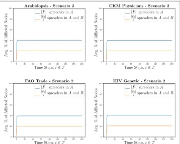
Real-world simulations

Results for real-world simulations depart from the general trend we observe in our synthetic simulations. In our real-world simulations, under designed initial spreader selection (Scenario 2), we observe that single-layer initial spreader generally outperforms multi-layer initial spreader selection. However, the important detail to note is that the difference is not as notable as with our synthetic simulations. Additionally, the propaga-tion process converges in a few time steps over the entire time horizonT. The amount of affliction that occurs varies based on value of. In Scenario 2-2, typically the affliction struggles to afflict additional nodes beyond the set of initial spreaders. However, in the other Scenarios considered, we see that affliction typically saturates at around 2·|F0|. The

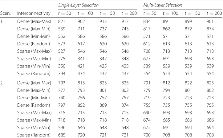
Table 4Heterogeneous data for whenNA=NB=500 and=3%

Single-Layer Selection Multi-Layer Selection

Scen. Interconnectivity t₌50 t₌100 t₌150 t₌200 t₌50 t₌100 t₌150 t₌200

1 Dense (Max-Max) 821 902 913 917 834 891 899 901

Dense (Max-Min) 539 711 737 743 817 862 872 874

Dense (Min-Min) 552 586 586 586 571 571 571 571

Dense (Random) 573 617 620 620 612 613 613 613

Sparse (Max-Max) 527 546 546 546 708 713 713 713

Sparse (Max-Min) 275 341 347 348 677 691 693 693

Sparse (Min-Min) 350 421 425 425 539 539 539 539

Sparse (Random) 394 434 437 437 554 554 554 554

2 Dense (Max-Max) 793 813 823 825 791 812 822 825

Dense (Max-Min) 777 793 801 802 779 794 801 802

Dense (Min-Min) 740 756 757 757 719 723 723 723

Dense (Random) 797 852 869 874 755 755 755 755

Sparse (Max-Max) 715 715 715 715 690 693 693 693

Sparse (Max-Min) 718 718 718 718 674 685 686 686

Sparse (Min-Min) 596 646 648 648 672 691 694 694

Sparse (Random) 685 720 721 721 700 708 708 708

time evolution of the propagation process for these real-world topologies can be seen in Fig.3.

The reasoning for this is likely due to the interconnection of the real-world topologies. It is very difficult to find publicly available M-IDN topologies. ComuneLab provides publicly available topological data for multiplex networks, from which we acquired real-world M-IDN topological data. However, a key distinction between the real-world topologies we run simulations on from this resource is that they aremultiplexnetworks. Refer to Table2 for an overview of the real-world multiplex topologies considered for this work.

Multiplex networks are topologies with numerous layers, with each nodes existing across every layer. These multi-layer network models allow for interesting relationships between entities. For instance, a layer in a multiplex network can have edges that rep-resent who retweets who on Twitter, while another layer in the same multiplex network can have edges that represent who replies to who on Twitter. In this example, each node is shared across each layer and inter-edges are only between each node to itself in every other layer. For instance, Donald Trump’s Twitter account would be a node shared across alllayers in a multiplex Twitter network. The inter-edges this node has will be to the other nodes representing Donald Trump’s Twitter account across all other layers. These nodes will havenointer-edges to nodes representing Twitter user accounts other than Donald Trump’s.

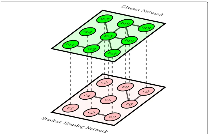
This detail is in stark contrast to our synthetic networks. We vary the level of interdependency across our synthetic topology through Sparse/Dense and Ran-dom/Designed interconnections. A visualization of what these topologies look like can be found in Fig. 4. Due to this high interconnection between layers, it makes sense that these networks do not exhibit the same behaviors of affliction as our synthetic topologies.

Degree single-layer vs. random multi-layer

For this work, we are interested in how designed, single-layer selection and random, two-layer selection compare. The interest in this is motivated by the notion that it is the-oretically easier to obtain topological structure of one layer within an M-IDN topology. With this knowledge, one could target highly connected nodes in this layer for affliction. With this in mind, we want to compare how a single-layer selection of initial spreaders by degree centrality (Scenario 1-2) compares to a two-layer selection of initial spreaders chosen at random (Scenario 2-1).

From analyzing the results from Tables4and3, we see that single-layer selection by degree centrality (Scenario 2-1) generally outperforms two-layer selection at random (Scenario 1-2) in both the heterogeneous and the homogeneous cases in the vast major-ity of experiments considered. However, it should be reiterated that single-layer selection selects nodes to be initial spreaders in layerA. With this in mind,kab=0.3 (andkba=0.8) for heterogeneous cases. The results of this analysis for the heterogeneous simulations depend largely on the inter-thresholds. If the inter-threshold values are sufficiently large, then Scenario 1-2 would very likely outperform Scenario 2-1.

Fig. 4Multiplex Network. An example of a two-layer multiplex social net- work where each node is represented in each layer. Each nodeiAhas an inter- edge to nodeiBand each nodeiBhas an inter-edge to

nodeiA. Layers “Classes Network” and “Student Housing Network” are social network layers where nodes

Conclusions

In closing, we studied how initial spreader selection strategies compare by analyzing the evolution of phenomena propagation over time using a state-of-the-art threshold-based propagation model. The benefit of our propagation model is that it is general enough to encapsulate other models of propagation (such as epidemic, linear probabilistic, lin-ear threshold, etc.). Our results show that, if you have knowledge about the topological structure (such as degree of nodes), multi-layer designed selection outperforms single-layer designed selection in most cases considered by our experiments. However, if you are in a situation where topological information is unavailable, random selection in a single-layer is more effective than multi-layer random selection. Additionally, from our work, we observe that single-layer selection by degree centrality (Scenario 2-1) generally outperforms two-layer selection at random (Scenario 1-2) most cases considered for this work.

Prior works investigating initial spreaders (or seed selection) in multi-layer networks are often interested in how phenomena propagation can be maximized or minimized given the context of the problem at hand (such as the influence maximization problem). In this work, our results are focused on analyzing how different interconnectivity cases and selection strategies with respect to layers considered for selection affect phenom-ena propagation. The general nature of our problem allows our work to provide insights to problems that aim to either maximize or minimize the overall affliction of a M-IDN topology as a result of phenomena propagation.

For future works in this direction, it is of interest to investigate the effectiveness of selec-tion strategies in M-IDN topologies consisting ofmlayers. With insight from how these varying strategies compare w.r.t. topological structure and interconnectivity, studying affliction in M-IDNs ofmlayers may be easier to investigate.

Endnotes

1_{We do not consider random (or designed) single-layer spread with phenomena initially}

spreading in because it is essentially the same scenario, since these are general network components.

2_{https://github.com/khamfroush-lab/initial-spreaders-project}

Abbreviations

BA: Barabási-Albert model for random graphs following a power law degree distribution; ER: Erd ˝os-Rényi model for random graphs; ICM: Independent cascade model; M-IDN: Multi-layer interdependent network; PLC: Programmable logic controller; SCADA: Supervisory control and data acquisition; WS: Watts-Strogatz model for random, small-world graphs

Acknowledgements

Not applicable.

Authors’ contributions

HK designed and formulated the problem, and proposed approaches to solve the problem described in this work. NH wrote the final draft of the paper for submission and analyzed results of experiments. SI ran simulations, documented results, and wrote an initial draft for the paper. MN collaborated with HK on formulation and simulation design and identifying the credibility of the problem formulation and simulations. All authors read and approved the final manuscript.

Funding

No outside funding was used to support this work.

Availability of data and materials

Ethics approval and consent to participate

Not applicable.

Consent for publication

Not applicable.

Competing interests

The authors declare that they have no competing interests.

Author details

1_{Department of Computer Science, University of Kentucky, University of Kentucky, Lexington 40506, KY, USA.}2_Electrical

Engineering Department, University of South Florida, E Fowler Ave, Tampa 33620, FL, USA.

Received: 6 November 2018 Accepted: 28 May 2019

References

Albert R, Jeong H, Barabási A-L (2000) Error and attack tolerance of complex networks. Nature 406(6794):378 Albright D, Brannan P, Walrond C (2010) Did Stuxnet Take Out 1,000 Centrifuges at the Natanz Enrichment Plant?.

Institute for Science and International Security. https://isis-online.org/isis-reports/detail/did-stuxnet-take-out-1000-centrifuges-at-the-natanz-enrichment-plant/

Anderson R, Fuloria S (2010) Who controls the off switch? In: 2010 First IEEE International Conference on Smart Grid Communications. IEEE, Gaithersburg. pp 96–101.https://doi.org/10.1109/SMARTGRID.2010.5622026.https:// ieeexplore.ieee.org/abstract/document/5622026

Barabási A-L, Albert R (1999) Emergence of scaling in random networks. Science 286(5439):509–512

Brooks R, Sander S, Deng J, Taiber J (2008) Automotive system security: challenges and state-of-the-art. In: Proceeding CSIIRW ’08 Proceedings of the 4th annual workshop on Cyber security and information intelligence research: developing strategies to meet the cyber security and information intelligence challenges ahead. ACM, New York. p 26.https://dl.acm.org/citation.cfm?id=1413170

Charles M, Grinstead J, Snell L (1997) Introduction to probability. Am Math Soc.https://bookstore.ams.org/iprob/ Checkoway S, McCoy D, Kantor B, Anderson D, Shacham H, Savage S, Koscher K, Czeskis A, Roesner F, Kohno T, et al. (2011)

Comprehensive experimental analyses of automotive attack surfaces. In: Proceeding SEC’11 Proceedings of the 20th USENIX conference on Security. USENIX, San Francisco. pp 77–92.https://dl.acm.org/citation.cfm?id=2028073 Chen W, Wang Y, Yang S (2009) Efficient influence maximization in social networks. In: Proceeding KDD ’09 Proceedings

of the 15th ACM SIGKDD international conference on Knowledge discovery and data mining. ACM, New York. pp 199–208.https://dl.acm.org/citation.cfm?id=1557047

Chen W, Wang C, Wang Y (2010) Scalable influence maximization for prevalent viral marketing in large-scale social networks. In: Proceeding KDD ’10 Proceedings of the 16th ACM SIGKDD international conference on Knowledge discovery and data mining. ACM, New York. pp 1029–1038.https://dl.acm.org/citation.cfm?id=1835934 Cohen R, Erez K, Ben-Avraham D, Havlin S (2001) Breakdown of the internet under intentional attack. Phys Rev Lett

86(16):3682

Coleman J, Katz E, Menzel H (1957) The diffusion of an innovation among physicians. Sociometry 20(4):253–270 De Domenico M, Nicosia V, Arenas A, Latora V (2015) Structural reducibility of multilayer networks. Nat Commun 6:6864 Erdos P, Rényi A (1960) On the evolution of random graphs. Publ Math Inst Hung Acad Sci 5(1):17–60

Erlandsson F, Bródka P, Borg A (2017) Seed selection for information cascade in multilayer networks. arXiv.org 689. https://link.springer.com/chapter/10.1007/978-3-319-72150-7_35

Halperin D, Heydt-Benjamin TS, Fu K, Kohno T, Maisel WH (2008) Security and privacy for implantable medical devices. IEEE Pervasive Comput 7(1):30–39.https://ieeexplore.ieee.org/abstract/document/4431854

Hanna S, Rolles R, Molina-Markham A, Poosankam P, Blocki J, Fu K, Song D (2011) Take two software updates and see me in the morning: The case for software security evaluations of medical devices. In: Proceeding HealthSec’11 Proceedings of the 2nd USENIX conference on Health security and privacy. USENIX Association, Berkeley.https://dl. acm.org/citation.cfm?id=2028032

Hoppe T, Kiltz S, Dittmann J (2008) Security threats to automotive CAN networks–practical examples and selected short-term countermeasures. In: International Conference on Computer Safety, Reliability, and Security. Springer. pp 235–248.https://link.springer.com/chapter/10.1007/978-3-540-87698-4_21

Hudson N, Turner M, Nkansah A, Khamfroush H (2019) On the effectiveness of standard centrality metrics for interdependent networks. In: 2019 International Conference on Computing, Networking and Communications (ICNC). IEEE, Honolulu.https://ieeexplore.ieee.org/abstract/document/8685586

Khamfroush H, Bartolini N, La Porta TF, Swami A, Dillman J (2016) On propagation of phenomena in interdependent networks. IEEE Trans Netw Sci Eng 3(4):225–239

Kandhway K, Kuri J (2017) Using node centrality and optimal control to maximize information diffusion in social networks. IEEE Trans Syst Man Cybern Syst 47(7):1099–1110

Kempe D, Kleinberg J, Tardos É (2005) Influential nodes in a diffusion model for social networks. In: International Colloquium on Automata, Languages, and Programming. Springer. pp 1127–1138.https://link.springer.com/chapter/ 10.1007/11523468_91

Kim H, Beznosov K, Yoneki E (2014) Finding influential neighbors to maximize information diffusion in twitter. In: Proceeding WWW ’14 Companion Proceedings of the 23rd International Conference on World Wide Web. ACM, New York. pp 701–706.https://doi.org/10.1145/2567948.2579358.https://dl.acm.org/citation.cfm?id=2579358

Kimura M, Saito K, Motoda H (2009) Blocking links to minimize contamination spread in a social network. ACM Trans Knowl Discov Data (TKDD) 3(2):9

McDaniel P, McLaughlin S (2009) Security and privacy challenges in the smart grid. IEEE Secur Priv 7(3):75–77.https:// ieeexplore.ieee.org/abstract/document/5054916

Metke AR, Ekl RL (2010) Security technology for smart grid networks. IEEE Trans Smart Grid 1(1):99–107 Michalski R, Kajdanowicz T, Bródka P, Kazienko P (2014) Seed selection for spread of influence in social networks:

Temporal vs. static approach. New Gener Comput 32(3-4):213–235

Mo Y, Kim TH-J, Brancik K, Dickinson D, Lee H, Perrig A, Sinopoli B (2012) Cyber–physical security of a smart grid infrastructure. Proc IEEE 100(1):195–209

Papanastasiou Y (2018) Fake news propagation and detection: A sequential model.https://papers.ssrn.com/sol3/Papers. cfm?abstract_id=3028354. Available at SSRN:https://ssrn.com/abstract=3028354orhttps://doi.org/10.2139/ssrn. 3028354

Pastor-Satorras R, Vespignani A (2001) Epidemic spreading in scale-free networks. Phys Rev Lett 86(14):3200 Rahman MA, Bera P, Al-Shaer E (2012) Smartanalyzer: A noninvasive security threat analyzer for ami smart grid. In: 2012

Proceedings IEEE INFOCOM. IEEE, Orlando. pp 2255–2263.https://ieeexplore.ieee.org/abstract/document/6195611. https://doi.org/10.1109/INFCOM.2012.6195611

Rushanan M, Rubin AD, Kune DF, Swanson CM (2014) Sok: Security and privacy in implantable medical devices and body area networks. In: 2014 IEEE Symposium on Security and Privacy. IEEE, San Jose. pp 524–539.https://ieeexplore.ieee. org/abstract/document/6956585.https://doi.org/10.1109/SP.2014.40

Salehi M, Sharma R, Marzolla M, Magnani M, Siyari P, Montesi D (2015) Spreading processes in multilayer networks. Netw Sci Eng IEEE Trans 2(2):65–83

Shu K, Bernard HR, Liu H (2019) Studying fake news via network analysis: detection and mitigation. In: Emerging Research Challenges and Opportunities in Computational Social Network Analysis and Mining. Springer. pp 43–65.https://link. springer.com/chapter/10.1007/978-3-319-94105-9_3

Stark C, Breitkreutz B-J, Reguly T, Boucher L, Breitkreutz A, Tyers M (2006) Biogrid: a general repository for interaction datasets. Nucleic Acids Res 34(suppl_1):535–539

Watts DJ, Strogatz SH (1998) Collective dynamics of ’small-world’networks. Nature 393(6684):440

Zhao D, Li L, Li S, Huo Y, Yang Y (2014) Identifying influential spreaders in interconnected networks. Phys Scr 89(1). https://iopscience.iop.org/article/10.1088/0031-8949/89/01/015203/meta

Publisher’s Note