Finding The Beta For A Portfolio
Isn’t Obvious: An Educational Example
James Chong, California State University, Northridge, USA William P. Jennings, California State University, Northridge, USA
G. Michael Phillips, California State University, Northridge, USA
ABSTRACT
When a portfolio is not actively managed to maintain a fixed investment percentage in each asset but rather maintains a fixed number of shares for each asset, the portfolio weights will change over time because the market returns of the different assets will not be the same. Consequently, portfolio betas computed as a linear combination of asset betas, which is the usual practice, will be different from betas computed using regression techniques on portfolio returns as is done when evaluating individual assets and mutual funds. The alternative approaches can result in quite different beta statistics and, consequently, inconsistent decisions depending on which method is used.
Keywords: Portfolio Beta; Risk; Measurement; CAPM
INTRODUCTION
his teaching note addresses a rarely discussed problem in financial pedagogy regarding the computation of portfolio “beta statistics”. While there is generally consensus in textbooks and professional literature regarding how to make this computation, there are inconsistencies in what is taught and underlying assumptions that are rarely discussed. This paper highlights those issues and provides a numerical example illustrating how the two different approaches to computing portfolio beta, sometimes viewed as equivalent in textbooks, provide quite different results.
Beta
A beta statistic is widely used in financial analysis to reflect the risk of an investment asset relative to a market benchmark. Finance, accounting, strategic management, and other areas of the business curriculum include beta to rank apparent riskiness in cash flows, to compute cost of capital, and to estimate various risk-adjusted performance statistics. Beta statistics are also popularly used as a constraint when constructing “Investment Policy Statements”, providing limits on acceptable beta statistics in investments or by outside managers. For example, Indiana University Foundation (2009) states that its “… equity (and REIT1) managers are expected to maintain a beta (vs. the primary benchmark) of less than 1.20.” Similarly, financial planners and wealth managers may compare the beta statistic for a client portfolio to a reported beta for a mutual fund or other investment product to determine if the fund is preferred to the stock portfolio.
METHODOLOGY
A common description of how to compute a portfolio beta is the one provided by Investorwords (2017), a top displayed search engine result, which states:
“Calculating your portfolio’s beta will give you a measure of its overall market risk. To do so, find the betas for all your stocks. Each beta is then multiplied by the percentage of your total portfolio that stock represents (i.e., a stock with a beta of 1.2 that comprises 10% of your portfolio would have a weighted beta of 1.2 times 10% or 0.12). Add all the weighted betas together to arrive at your portfolio’s overall beta.”
1REIT stands for real estate investment trust.
The beta statistic is viewed as linear, so that the portfolio beta is the linear combination of the component asset betas and the weights are corresponding asset weights in the portfolio. What is not stated, but is clearly implied, is that the asset weights are those at the time the linear combination is performed. And, that’s the problem. When a portfolio is not actively managed to maintain a fixed percentage in each asset but rather maintains a fixed number of shares for each asset, the portfolio weights will change over time because the market returns of the different assets will not be the same. Most Individual Retirement Account (IRA) and personal accounts and endowment funds holding individual stocks maintain fixed shares, not fixed percentages, of their investments.
The most frequently discussed alternative to find beta statistics is to apply linear regression to the historical values of the portfolio. The regression may be applied to portfolio values with changing holdings or to a “pseudo portfolio” based on historical values of current holdings with current share positions. For example, Alexander (2001) states
“An artificial history of portfolios returns is constructed using the current portfolio weights and historic data on each asset. Alternatively, the individual stock betas may be weighted by the proportion of the funds that is invested in stock with return y, denoted wy. Then summation gives the net beta of the portfolio as βY = Σ wyβy. When ordinary least squares is used to estimate the betas the two methods will give the same results.”
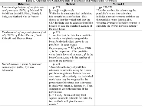
A digest of several representative textbooks and professional references presenting what is said about computing portfolio beta statistics is presented in Table 1, showing that most definitions use the weighted average approach, some discuss the regression approach, but both methods are viewed as interchangeable.
Table 1. Approaches to Computing Beta in Textbooks and Professional References
Reference Method 1 Method 2
Investments principles of portfolio and equity analysis (2011) by Michael G. McMillan, Jerald E. Pinto, Wendy L. Pirie, and Gerhard Van de Venter
p. 271
βp = w1β1 +w2β2 +w3β3
While this is a mathematical definition, it is nonetheless a definition. This shows us that the typical path that the CFA Institute uses to calculate portfolio betas is to take the weighted average of the asset betas.
pp. 271-272
“Another method for calculating the portfolio’s return is to calculate individual security returns and then use the portfolio return formula (i.e., weighted average of security returns) to calculate the overall portfolio return.”
Fundamentals of corporate finance (3rd ed.) (2015) by Robert Parrino, David Kidwell, and Thomas Bates
p. 229
“…we find that the beta for a portfolio is simply a weighted average of the betas for the individual assets in the portfolio. In other words:
𝛽" $%%&' ()*'+),-)= ∑"-12𝑥-𝛽-… where
𝑥- is the proportion of the portfolio
value that is invested in asset i, 𝛽- is the
beta of asset i, and n is the number of assets in the portfolio.”
Market models: A guide to financial data analysis (2001) by Carol Alexander
p. 231
“An artificial history of portfolios returns is constructed using the current portfolio weights and historic data on each asset. Alternatively, the individual stock betas may be weighted by the proportion of the funds that is invested in stock with return y, denoted wy. Then summation gives the net beta of the portfolio as
βY = Σwyβy. When ordinary least squares is used to estimate the betas the two methods will give the same results.”
(Table 1 continued)
Reference Method 1 Method 2
Handbook of portfolio construction: Contemporary application of Markowitz techniques (2010) by John B. Guerard, Jr., editor
p. 34
Beta is simply referred to as, “security beta, a random regression coefficient.”
Investment valuation: Tools and techniques for determining the value of any asset (2nd ed.) (2002) by Aswath Damodaran
p. 78
“…the beta of a portfolio is the weighted average of the betas of the assets in the portfolio. This property in conjunction with the absence of arbitrage, leads to the conclusion that expected returns should be linearly related to betas.”
p. 120
“The beta (if using a single-factor model) or betas (if using a multifactor model) of each portfolio are estimated, either by taking the average of the betas of the individual stocks in the portfolio or by regressing the portfolio’s returns against market returns over a prior time period (for instance the year before the testing period.”
Quantitative equity portfolio management: An active approach to portfolio construction and management (2006) by Ludwig B. Chincarini and Daehwan Kim
pp. 474-475
“A performance analyst can find β
either by taking the weighted average of the β’s of each stock in the portfolio…” or by running a linear regression of the portfolio’s returns against the market’s returns.
pp. 474-475
“…or by running a linear regression of the portfolio’s returns against the market’s returns.”
Modern portfolio theory and investment analysis (7th ed.) (2007) by Edwin J. Elton, Martin J. Gruber, Stephen J. Brown, and William N. Goetzmann
p. 137
“Define the Beta on a portfolio βp as a weighted average of the individual βis on each stock in the portfolio where the weights are the fraction of the portfolio invested in each stock. Then 𝛽(=
∑"-12𝑋-𝛽-”
Investment: Concepts, analysis, and strategy (5th ed.) (1997) by Robert C. Radcliffe
p. 268
“The beta of a portfolio can also be calculated as a weighted average of the betas on the securities that make up the portfolio: 𝐵(= ∑"-12𝛽-𝑥-”
pp. 267-268
“There are two ways of calculating the beta of a portfolio: (1) at the portfolio level, or (2) at the component security level. At the portfolio level, the beta is simply:
Βp = σprpM/σM
The standard deviation of the portfolio returns is divided by the standard deviation of the market portfolio to find the amount of uncertainty in the portfolio relative to the market portfolio’s uncertainty. This value is then multiplied by the correlation between the portfolio and the market portfolio to determine what portion of the relative uncertainty will not be diversified away when the portfolio is held.”
DISCUSSION
Consider a buylist comprised of 30 very large publicly traded companies. A list of such companies with their recently estimated beta statistics (using one-year daily returns) is provided in Table 2.
Table 2. Beta of 30 Publicly Listed Companies as of February 1, 2017
Name Symbol Beta Statistic
J P Morgan Chase & Co JPM 1.4754
Apple Inc AAPL 0.8816
Johnson & Johnson JNJ 0.4532
McDonald’s Corp MCD 0.5108
Boeing Co (The) BA 1.1732
Verizon Communications Inc VZ 0.5082
Coca-Cola Co (The) KO 0.6246
International Business Machines Corp IBM 1.0047
Walt Disney Co (The) DIS 0.7970
Procter & Gamble Co (The) PG 0.5297
Home Depot Inc (The) HD 0.8721
Exxon Mobil Corp XOM 0.7634
Pfizer Inc PFE 0.7645
Merck & Co Inc MRK 0.9096
American Express Co AXP 1.1097
Microsoft Corp MSFT 1.1877
Cisco Systems Inc CSCO 0.9891
Nike Inc NKE 0.9308
Intel Corp INTC 1.1990
Caterpillar Inc CAT 1.4566
3M Co MMM 0.7192
E.I. du Pont de Nemours and Co DD 0.9373
General Electric Co GE 0.9966
Wal-Mart Stores Inc WMT 0.4389
Chevron Corp CVX 1.0767
United Technologies Corp UTX 0.9221
Goldman Sachs Group Inc (The) GS 1.5544
UnitedHealth Group Inc UNH 0.8213
The Travelers Companies Inc TRV 0.7832
VISA Inc V 1.1984
What is the portfolio beta for an equally weighted portfolio of these 30 stocks? Using the approach that says the portfolio beta is a weighted average of asset betas, and since there are equal weights for these stocks, the portfolio beta is just the arithmetic mean of these 30 stocks:
βY = Σ wyβy = Σ (1/30)βy = (Σβy)/30 (1)
Evaluated at the beginning of 2017, the “textbook portfolio beta” value is found to be 0.9196.
However, suppose that the historical values of the portfolio were used in a linear regression to find the portfolio beta, using the same method taught for finding individual asset beta statistics. While the portfolio is designed to have the number of shares of each stock that would result in equal weighting in 2017, those shares would have changed in value over time so that portfolio weights at different dates would be different even though the total number of shares of each asset was constant. This is easily done by computing the total value of the time series of the individual stock prices weighted by the number of shares for each stock. (The constant shares approach is in contrast to the constant percentage method in which the weighted average of individual stock returns, not market values, is computed.)
In this case, the two estimates differ by almost 3%. Were an individual’s portfolio beta computed using the “textbook portfolio beta” approach compared to a time-weighted mutual fund beta of similar strategy, the mutual fund would appear to be relatively safer than the individual portfolio. However, that would be an artifact of the method for computing beta.
This observation also has application to financial decision making. To illustrate the practical significance of the numerical difference shown above, consider using beta in the Capital Asset Pricing Model (CAPM) for computing a discount rate (K = riskless rate of interest + beta × market risk premium). Suppose that the market risk premium is assumed to be 8% and the riskless rate of interest is 2%. The two discount rate possibilities with the constant percentage weights and constant share beta estimates are:
K = 0.02 + 0.9196 × 0.08 = 9.3568% (constant weights)
K = 0.02 + 0.8937 × 0.08 = 9.1496% (constant shares)
While 9.3568% and 9.1496% might seem numerically close, even these “small” differences have significant impact on valuation. For example, the present value of a $10 perpetuity (like preferred stock or a console bond) would be $106.87 (= 10/0.093568) with constant weights and $109.29 (= 10/0.091496) with constant shares. A measure of the economic significance of these pricing differences is the “bid-ask spread” for stocks in the marketplace. A recent Vanguard (2017) report stated that the bid-ask spread for its S&P 500 exchange-traded fund (ETF) was approximately 1 basis point (0.01%, also written as 1 bps), with other funds’ bid-ask spreads ranging from an average of 5 bps to a high of about 23 bps. Similarly, Securities and Exchange Commission (2016) microstructure analysis refers to stock spreads from about 11 bps on the New York Stock Exchange (NYSE) to as high as 120 bps on the Nasdaq Stock Market for some stocks. These observed spreads highlight that the difference in valuation brought by alternative computational techniques for the beta statistic can be substantially larger than normal differences in valuation observed in the market.
Which is the “correct” method for computing beta? That answer depends on the desired application of the beta statistic. For purposes of portfolio analysis and risk documentation, the time-weighted beta computed by finding the actual portfolio returns over time and relating those to benchmark returns, reflects the riskiness inherent in whatever strategy is pursued to manage the portfolio and is directly comparable to the estimated beta statistics for traded funds and separately managed portfolios.
If a portfolio is to be compared to a constantly reweighted portfolio designed to maintain constant portfolio weights, such as an index fund, then the traditional textbook “constant portfolio weight” (varying shares) approach is computationally similar. An argument can be made for using the traditional method when looking forward, by saying that the past weights in the portfolio are over and the current weighting is what the investor is concerned with now. However, if going forward the portfolio is periodically reweighted according to an algorithm or according to some consistent asset allocation strategy, then the time-weighted (constant share) approach reflecting the actual changes made to the portfolio, if any, could be more predictive of future performance.
As a further teaching point, all of the above differences can be applied to dual beta models in which separate up-market and down-up-market beta estimates are computed and symmetric response to benchmarks is not assumed. The topic of dual betas is further developed in Chong, Pfeiffer, and Phillips (2011), Chong and Phillips (2011), Chong, Halcoussis, and Phillips (2012), Chong and Phillips (2012), Chong, Jennings, and Phillips (2013), and Chong, Jin, and Phillips (2014).
CONCLUSION AND TEACHING POINTS
important when the resulting portfolio statistic is used to compare a portfolio to a managed alternative such as a mutual fund or index fund, or when used to estimate an offer price for another traded portfolio assets. Using standard tools, students can estimate how beta statistics for a portfolio would differ when using both computational methods. Comparing estimated beta statistics to reported statistics for index funds allows for significant class discussion regarding the impact of rebalancing on portfolio characteristics and, when fees are included, on overall return.
DECLARATION OF CONFLICTING INTERESTS
The authors declared no potential conflicts of interest with respect to the research, authorship, and/or publication of this article.
ACKNOWLEDGEMENTS
The authors wish to thank Laurel Fish for research assistance.
AUTHOR BIOGRAPHIES
James Chong is a Professor and Associate Director of the Center for Financial Planning and Investment at California State University, Northridge. He also serves as a Research Economist at MacroRisk Analytics. He received his Ph.D. in Finance from ICMA Centre, The University of Reading.
William P. Jennings is a Professor of Finance and Dean Emeritus of Business at California State University, Northridge, where he was formerly Chair of the Department of Finance, Financial Planning, and Insurance. He received his Ph.D. in Economics from the University of California, Los Angeles.
G. Michael Phillips is the Director of the Center for Financial Planning and Investment and a Professor of Finance, Financial Planning, and Insurance at California State University, Northridge. He also serves as Chief Scientist for MacroRisk Analytics. He received his Ph.D. from the University of California, San Diego, with specializations in econometrics and applied economics.
REFERENCES
Alexander, C. (2001). Market models: A guide to financial data analysis. John Wiley & Sons, Ltd.
Chincarini, L. B., & Kim, D. (2006). Quantitative equity portfolio management: An active approach to portfolio construction and management. McGraw-Hill Companies, Inc.
Chong, J., Halcoussis, D., & Phillips, G. M. (2012). Misleading betas: An educational example. American Journal of Business Education, 5(5), 617-622.
Chong, J., Jennings, W. P., & Phillips, G. M. (2013). Why downside beta is better: An educational example. American Journal of Business Education, 6(3), 371-374.
Chong, J., Jin, Y., & Phillips, G. M. (2014). The entrepreneur’s cost of capital: Incorporating downside risk. Business Valuation Review, 33(3), 81-91.
Chong, J., Pfeiffer, S., & Phillips, G. M. (2011). Can dual beta filtering improve investor performance? Journal of Personal Finance, 10(1), 63-86.
Chong, J., & Phillips, G. M. (2011). Beta measures market risk except when it doesn’t: Regime switching alpha and errors in beta. The Journal of Wealth Management, 14(3), 67-72.
Chong, J., & Phillips, G. M. (2012). Measuring risk for cost of capital: The downside beta approach. Journal of Corporate Treasury Management, 4(4), 344-352.
Damodaran, A. (2002). Investment valuation: Tools and techniques for determining the value of any asset (2nd ed.). New York, NY: Wiley & Sons, Inc.
Elton, E. J., Gruber, M. J., Brown, S. J., & Goetzmann, W. N. (2007). Modern portfolio theory and investment analysis (7th ed.). John Wiley & Sons, Inc.
Guerard, J. B., Jr. (Ed.). (2010). Handbook of portfolio construction: Contemporary application of Markowitz techniques. Springer.
Investorwords. (2017). Calculating your portfolio’s beta. Retrieved from http://www.investorwords.com/tips/271/calculating-your-portfolios-beta.html
McMillan, M. G., Pinto, J. E., Pirie, W. L., & Van de Venter, G. (2011). Investments principles of portfolio and equity analysis. Hoboken, NJ: John Wiley & Sons, Inc.
Parrino, R., Kidwell, D., & Bates, T. (2015). Fundamentals of corporate finance (3rd ed.). John Wiley & Sons, Inc. Radcliffe, R. C. (1997). Investment: Concepts, analysis, and strategy (5th ed.). Addison-Wesley Educational Inc.
U.S. Securities and Exchange Commission. (2016). Corporate stock trading volume, spreads and depth before, during and after the NYSE trading suspension on July 8, 2015. Retrieved from https://www.sec.gov/marketstructure/research/highlight-2016-01.html#.WKtW33_ctv8