EFFECT OF BENDING RIGIDITY OF MARINE CABLES ON THE DYNAMIC STABILITY OF TWO-PART UNDERWATER TOWING SYSTEM

EFFECT OF BENDING RIGIDITY OF

MARINE CABLES ON THE DYNAMIC

STABILITY OF TWO-PART

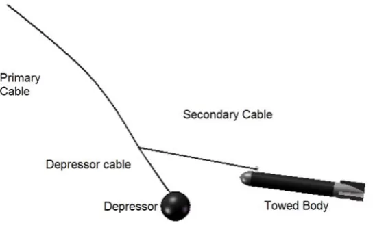
UNDERWATER TOWING SYSTEM

LALU P.P

Research Scholar, Department of Ship Technology , Cochin University , Kalamassry, Kerala, India Ph 00919447921327 , Email: [email protected]

Dr K.P Narayanan

Reader, Department of Ship Technology , Cochin University , Kalamassry Kerala, India

Abstract :

The study mainly focuses on the motion dynamics of a two-part under water towing system which is used to tow acoustic instrumentations for ocean exploration and naval defense. During the towing process, the disturbances from the ship travel down to the cable and to the towed body resulting in the oscillation of the same. This will lead to the lower performance of the acoustic instrumentation inside. Hence estimation of the amount of these oscillations is the main objective of the study. For this, dynamic simulation was used which consists of cable modeling and vehicle formulation. Previous studies in this direction used a lumped mass spring model for the cable which completely ignores the bending rigidity of the cable. Hence the this paper mainly estimates effect of bending rigidity of the tow-cable on the dynamic stability of two-part towing system using an improved lumped mass spring formulation. The simulated values are compared with experimental values obtained from the literature.

Keywords: Marine Cable, Dynamics, Towing.

1. Introduction

Historically, two methodologies were evolved for modeling the cable. Theses are segmental approach and lumped mass approach. For the former, the cable is modeled as continuous system and resulting partial differential equations are solved by finite difference or any suitable approximation method. In lumped mass-spring system, the cable is discretised at the very beginning of the model and is replaced by point masses joined

together by mass-less elastic elements of finite length. Thus the discretised model consists of many point masses and mass-less elastic strings. All the forces along the cable are assumed to be concentrated at the mass points. Existing method utilises segmental approach which is found very difficult to implement. On the other hand lumped mass formulation is simple and easy to implement. Thus the present study utilises the lumped mass formulation for the modeling of the cable.

Out of the various lumped mass formulations for the cable, the method proposed by Shan Huang [7] is promising. But limitation of this lumped-mass-spring model is that it does not have bending rigidity in the cable formulation. Therefore the model is best suited for long cables having small diameter (i.e negligible bending rigidity). But in two-part towing system this cannot be ignored as secondary and depressor cable are considered to be very short compared to primary cable. Hence the present study attempts to include the bending rigidity in the cable formulation using LMSM to simulate the dynamics of two-part towing system.

2. Lumped Mass spring model with bending rigidity

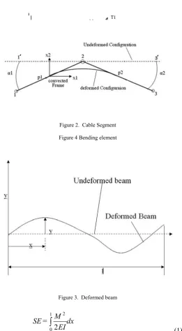
Figure 2 shows a small segment of the cable. T and M represent cable tension and bending moment respectively. For the two-dimensional element, the only moment balance involves moments about the out-of-plane axis. The tension force does not contribute a moment in this case because in the infinitesimal limit the tangential and normal directions at the two opposite ends have the same direction and opposite magnitudes. The remaining moment contributions are the rotational inertia, the couple due to bending of the element.

In segmental formulation the independent variables to be considered are space, tension, moment and slope at the two ends (θ1 and θ2). This would results in large number of degrees of freedom to be solved as the number of degrees of freedom per node is considerably large. To avoid this, a modified beam model which is having lesser degrees of freedom per node has been used in this particular study. Thus all the equations to be assembled, remain to be that of translational degrees of freedom rather than rotational and translational mix. This would avoid the assemblage of momentum balance equation for each segment. The formulation has been discussed in detail in the literature [9] where it was mainly used to simulate the flexible dynamics of spatial mechanisms.

Suppose we have an originally undeformed straight beam of length l (figure 3) .Let x be the co-ordinate along the neutral axis of the undeformed beam and y be the co-ordinate of the transverse distance between the original undeflected shape of the beam and the deformed shape. The total strain energy neglecting the shear deformation of the beam according to the Euler beam theory is given by

dx EI M = SE

_

1

0 2

2 ₍₁₎

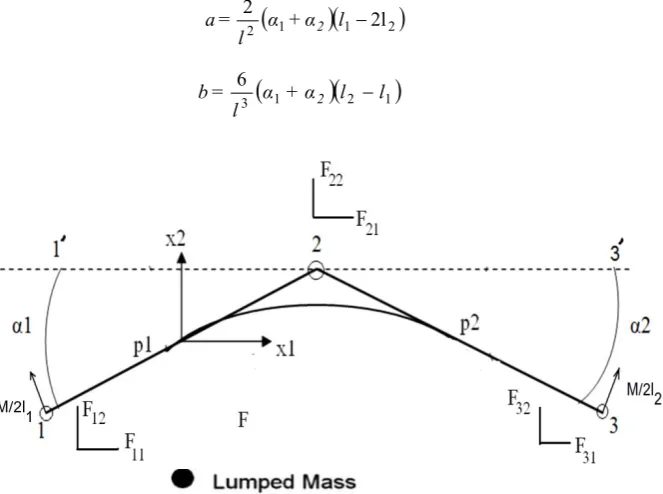
Where E is the Young’s modulus, I is the moment inertia of the cross-section in the transverse direction and M is the bending moment. To obtain the axial response of the modified element, two truss elements are inserted between nodes 1 and 2 and nodes 2 and 3 (Figure 4). Subsequently, a torsion spring was inserted at node 2 to provide bending rigidity. Hence the improved cable model is shown in the figure 5.

In the literature [9] it has been shown that





3

2 ₃

3a

6 l+ abl +b l

EI =

SE 2 2

(2) Figure 2. Cable Segment

2



1



1 2l2



2 _ l α + α l = a ₂ (3a) 6₃



α₁+α



l₂ l₁



l =

b ₂  (3b)

Where l1 is the distance between nodes 1 and 2. Similarly l2 = distance 2-3 Assuming ll = l2 = l/2 and α1 = α2 = α/2;

 

2 2 1 α l EI = SE       (4) This equation represents strain energy stored in a torsion spring with stiffness kb given by

kb = EI/l (5) The equivalent lumped nodal forces due to moment produced at the nodes are given by

                                                     2 2 2 2 2 2 1 1 2 2 1 1 1 1 1 1 3,2 3,1 2,2 2,1 1,2 1,1 / cos / sin / cos / cos / cos / sin / cos / sin 2 / l ) (α l ) (α l ) (α + l ) (α l ) (α + l ) (α l ) (α l ) (α M = F F F F F F = Fe

i (6)

The free body diagram with equivalent nodal forces is shown in figure 6.

3. Equation of motion of the Cable

The discretised cable model (figure 5) consists of many point masses, mass-less linearly elastic springs and torsion springs. The governing equations of cable excluding that of the torsion spring are described in detail in the literature [7]. All the forces along the cable are assumed to be concentrated at the mass points, which are numbered by i, which ranges from 1 to N. The lumped mass consists of mass of the cable as well as the added mass. By invoking Newton’s laws of motion [7] for the ith _{node on the line as shown in figure 2}

(Mi + ei)ai = Fi (7) Where Mi and ai are the lumped mass and acceleration at the node i and the ei is the contribution of the added mass. The external force Fi is the sum of cable tension, hydrodynamic drag, buoyancy, gravitational force and structural forces generated due to torsion springs.

4. Boundary condition

Boundary condition must be given at the top end of the primary cable, at the depressor and at the tow-fish. Additional boundary condition must be enforced at the junction of the three cables. The boundary condition at the top end was determined by the known ship motion. The depressor was assumed to be weighted ball. Sy and Sz are the projected area of the depressor along the plane perpendicular to Y and Z-axis respectively. Cdy and Cdz are the corresponding drag coefficients. The equation of motion for the depressor is formed based on the Newton-Euler formulation

                  

  

z0 y0

F F = z y a a

 

22 11

0

0 ( 8)

Where a11 = M0 + m0 + May and a22 = M0 + m0 + Maz

Where m0 = added mass of the cable segment and M0 = mass of the Depressor May and Maz are the contribution of added mass along Y and Z direction respectively

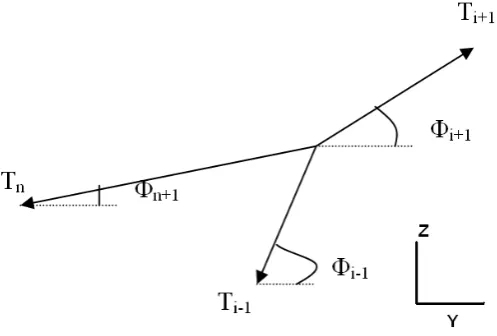
T is the tension in cable near the depressor. The external forces Fy0 and Fz0 include the effects due to drag of the depressor, cable and gravitational and buoyancy of the same. The boundary condition at the junction of the three cables is shown in figure 7. The Newton’s law was invoked at the junction of three cables as in the earlier case but the lumped mass as well as the forces include the contribution from primary, secondary and depressor cable.

_

F_y=T_i+1cosφ_i+1T_i1cosφ_i1T_n+1cosφ_n+1 ( 9)

_

F_z=T_i+1sinφ_i+1T_i1sinφ_i1T_n+1sinφ_n+1 (10) Where Ti+1andTi-1 are the tension at the i+1 and i-1 nodes respectively.

To complete the formulation a set of initial condition must be specified for each node in the line. This includes both initial position and initial velocities, as required second order ordinary differential equations.

y

_i



a

;

y



_i



b

;

z

i



c

;

z



i



d

;

For all i = 0,1,2...n; (11)

5. Finite Difference Implementation

The time domain is divided into a set of discrete steps t = jδt,(j = 1 ,2 3,...). Assuming every thing is known at

previous time step t = jδt, the question is how to find out the unknowns at the next time step t = (j+1) δt through the governing equations complemented by boundary condition.

y



y_ij+ +y_ij y_ij



Δt

= 1 1 1 2

2 ..



 ₍₁₂₎

y. 1



y_ijy_ij1



Δt

= (13) We can now approximate governing equation (7) at the time step t by using the above difference equations. Finally there are 2N algebraic equations for 2N unknowns. The tension is now calculated by using linearly elastic assumption once the solution of the 2N unknowns is obtained. The assembled equations are solved using a nonlinear solver.

6. Kinematics and Dynamics of the Tow-fish

The kinetic and kinematic equations of motion are derived based on a right-handed orthogonal coordinate system, which is fixed, at the center of buoyancy of the body. This is assumed to be approximately, at the geometric center of the body. Also rigid body dynamics is assumed through out. The equations of motion of the same are discussed in literature [3, 8].

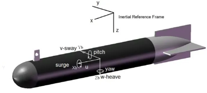
Figure 8 shows the possible motions of a towed body. This includes three rotary motions namely pitch, heave and roll and three translatory motions namely surge, heave and sway. As shown in the figure axes xb and zb lie in the plane of symmetry containing the rudder. The xb axis points out of the nose; yb axis completes the right-handed reference frame.

The variable XI = [x, y, z]T _{is the tow-fish position relative to an inertial frame,}

ΦI = [ φ, θ, ψ]T _{are the Euler angles representing the tow-fish attitude with respect to the inertial frame.} V = [u, v, w] T _{is the velocity represented in the body fixed frame}

Ω= [p, q, r] T _{is the tow-fish angular velocity with respect to the axes represented in the body frame. The state} of the towed body can be written as follows

X = [ Xl ,Φl,V,Ω]T ₍₁₄₎ The transnational kinematic equation is

.

Where R =





























































































c

c

s

c

s

c

s

s

s

c

s

s

s

c

c

c

s

s

c

c

s

s

s

s

c

c

s

c

c

(16) Where symbols ‘s’, ‘c’ and ‘t’ means sine, cosine and tangent respectively. The rotational kinematic equation is

                                     r q p c c c s s c t c t s



























/ / 0 0 1 . . . (17)

The contribution of added mass is also included in the rigid body mass. Hence the mass matrix becomes

               

Z

k

Y

k

k

wf vf m m m M ) 1 ( 0 0 0 ) 1 ( 0 0 0 ) 1 ( 2 2 1 (18)

Where k1, k2 and k3 are the coefficient of added mass in the three direction x, y and z. Yvf and Zwf are the added mass contribution of the fin towards y and z directions. The rigid body moment of inertia and added inertia matrix for the towed body is









                    

N

k

I

I

I

I

M

k

I

I

I

I

K

I

rf z yz xz yz qf y xy xz xy pf x J 3 3 1

1 (19)

The Mqf Nrf and Kpf are the added mass contribution due to fins. This matrix D represents the inertial coupling between the translational and rotational motion [3].

7. Motion Dynamics

Kirchhoff’s equations for motion of a rigid body in an ideal fluid, generalized to include exogenous forces and torques, are [8]









_                            

M

D

F

D

D

ext T ext T T V MV DV J MV V J D M   (20) Fext and Mext are the external force and moment vectors defined as



_F

_F

_F

_F

_F



F

F

F

F

body tail tow weight buoyancy

normal lateral axial

external     

         

 (21)



_M

_M

_M

_M

_M



M

M

M

M

body tail tow damping weight

Yaw pitch

roll

external     

         

 (22)

Equation 20 represents the final equation of motion of the tow-fish. The external forces and moments has to be estimated separately. Also the connecting equation for the cable termination and tow point of the body was given by

8. Numerical simulation

For the demonstration of the developed model, a numerical example of the towing ship traveling in a wave field is described here. Only two-dimensional simulation is attempted. The towing ship travels sinusoidally on the horizontal plane with horizontal velocity V0. Subsequently the simulated data are compared with the experimental values obtained from the literature [11]. Because of the limitation in the availability of the experimental values only heaving is compared

Wu et.al [11] conducted experiments to study the performance of the two-part underwater towing system. To simulate the phenomenon of a towing ship traveling in wave field, he devised a slider crank mechanism which provides excitation at the end of the primary cable. A pressure based depth sensor has been devised to measure the heave response of the towed body. Similarly the pitch was measured using accelerometer. The real time tension at the primary cable was also recorded. The experiments were conducted under the conditions of straight towing with constant towing speed and an excitation at the top end of the primary cable which is impelled by slider crank mechanism.

Thus heave amplitude of the tow point is given by

    

  

      

        

 t

T l

t T r

l

r

z

p





2

1 1 2

cos

_sin

2

2 2

(24)

Where r and T are the length and rotation period of the crank and l is the length of the connecting link for the slider crank mechanism. The value for the above is discussed in table 1. Three Φ2mm steel wire ropes were used as primary, secondary and tertiary cables. The depressor used in his experiment was a steel sphere of diameter 0.11m and 5.25 kg weight in water. The towed tow-fish is built by using circular nylon cylinder 0.11m in diameter and 2mm in thickness. The tow-fish was adjusted to be neutrally buoyant and the tow point is fixed at left end point of the tow-fish. Also, the towed body was adjusted to be floating upright in water by placing ballast weight.

Table 1

V0 (m/sec) L(m) T (sec) r(m)

1.75 0.35 1.6 0.1

The particulars of composite cables, depressor and towed tow-fish system are Depressor :-Diameter = 0.11m Weight in air = 5.25kg. Weight in water = 4.58 kg.

Towed Tow-fish:- Diameter = 0.11m. Length = 1.30m. Weight in air 12.50. weight in water = 0 kg. Primary cable:- length 2.84m. Weight in air = 0.181 kg/m. Weight in water = 0.104kg/m.

Depressor Cable:- Length = .30m weight in air = .063 kg/m. Weight in water = 0.039kg/m Secondary cable :-Length = 1.5m. Weight in air 0.124kg/m.Weight in water = 0.065 kg/m

The equations of tow-fish are simplified to two-dimensional. For simplicity no fin is taken into consideration. As the total mass and distance between the center of gravity and center of buoyancy (Where the local coordinate system is fixed) of the towed body and is very small the coupling relation of mass terms (matrix D) is neglected. 9. Results and Discussion

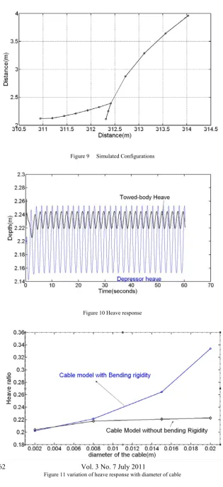
Figure 10 shows the simulated time based heave data of the depressor and towed body. It can be seen that the heave response of the towed body is considerably less than that of the depressor. Also the input disturbance from the ship is considerably scaled at the towed body end. The simulated heave amplitude ratio is found to be approximately 0.2021. The same ratio obtained from the experimental values from literature [11] is found to be 0.23.

Figure 9 Simulated Configurations

Figure 11 shows the variation of heave ratio with respect to the diameter of the cable. In the first case the bending rigidity of the cable was also taken into consideration in the lumped mass spring model and in the second case the same was absent while keeping all parameters the same. It can be seen that when the diameter of the cable is low (up to 8mm), the predicted heave ratio by the two models are equivalent. But as the diameter increases further, this value differs considerable for the two models. This may be due to the enhanced bending rigidity (EI) at higher diameter of the cable. Thus it may be concluded that the bending rigidity of the cables plays a significant role in the motion stability of two-part towing system. As the cables diameter increases, it becomes stiffer results in the increase of the heave amplitude. This may make the body becomes unstable. So a highly flexible cable is suggested for the underwater towing process for the better stability of the towed vehicles.

10. Conclusion

The two-part system discussed above is an innovative towing system to enhance the stability of underwater acoustic instrumentations. The lumped mass spring model described above is capable of modeling two part towing system with ship disturbances as input. At lower diameters the simple lumped-mass-spring system and proposed model gives almost same results. But for larger diameter cables, there is considerable deviation in the heave ratio for the two models. Therefore lumped mass spring model with bending rigidity of the cable being considered is more versatile than simple lumped mass spring model. Also, the bending rigidity of the cables plays a significant role in the motion stability of two-part towing system. So a highly flexible cable is suggested for the underwater towing process for the better stability of the towed vehicles. The numerical simulation it is revealed that two part towing system is efficient in reducing the heaving response of the tow-fish.

References:

1. Ablow C M & Schechter, S ”Numerical Simulation of Undersea Cable Dynamics”, Ocean Engineering, Vol.10, No.6, pp 443-457,1983.

2. Chapman D.A “Towed Cable Behavior During Ship Truing Maneuvers” , ”, Ocean Engineering, Vol. 1,No.4, pp.327-361, 1984. 3. Eric M Schuch , “Tow fish Design and Control”, PhD thesis Virginia Polytechnic Institute. 2004.

4. Gobat I.J, ‘Dynamics of geometrically compliant mooring system’, PhD Thesis, Department of Ocean engineering MIT,USA, 2000. 5. Hughes T.J.R, Finite Element Method, Prentice Hall Inc, New Jersey.

6. Ranmuthugala, S.A Gottschalk, “Investigation into two-part underwater tow”, proceedings of first international conference on underwater tow, Wuxi, China, pp 663-670, 1994.

7. Shan Huang, ”Dynamic Analysis of Three Dimensional Marine Cables”, Ocean Engineering, Vol. 21,No.6, pp.587-605, 1994. 8. Thor I Fossen, “Guidance and Control of Ocean vehicles” John Wiley and Sons, 1994.

9. Wasfy T M, ‘A torsional spring like beam element for the dyanamic analysis of flexible muti-body systems’, Intl. Jou. of Num. Methods in Engg, 39(1996) pg 1079-1096.

10. Wu J, A.T Chwang, “A Hydrodynamic Mode Of A Two-Part Underwater Towing System” ,. Ocean Engineering, Vol. 27, pp.455-472, 2000.