Essays In Causal Inference: Addressing Bias In Observational And Randomized Studies Through Analysis And Design

University of Pennsylvania

ScholarlyCommons

Publicly Accessible Penn Dissertations

2019

Essays In Causal Inference: Addressing Bias In

Observational And Randomized Studies Through

Analysis And Design

Raiden Berte Hasegawa

University of Pennsylvania, [email protected]

Follow this and additional works at:

https://repository.upenn.edu/edissertations

Part of the

Statistics and Probability Commons

This paper is posted at ScholarlyCommons.https://repository.upenn.edu/edissertations/3365

Recommended Citation

Hasegawa, Raiden Berte, "Essays In Causal Inference: Addressing Bias In Observational And Randomized Studies Through Analysis And Design" (2019).Publicly Accessible Penn Dissertations. 3365.

Essays In Causal Inference: Addressing Bias In Observational And

Randomized Studies Through Analysis And Design

Abstract

In observational studies, identifying assumptions may fail, often quietly and without notice, leading to biased causal estimates. Although less of a concern in randomized trials where treatment is assigned at random, bias may still enter the equation through other means. This dissertation has three parts, each developing new methods to address a particular pattern or source of bias in the setting being studied. In the first part, we extend the conventional sensitivity analysis methods for observational studies to better address patterns of heterogeneous confounding in matched-pair designs. We illustrate our method with two sibling studies on the impact of schooling on earnings, where the presence of unmeasured, heterogeneous ability bias is of material concern. The second part develops a modified difference-in-difference design for comparative interrupted time series studies. The method permits partial identification of causal effects when the parallel trends assumption is violated by an interaction between group and history. The method is applied to a study of the repeal of Missouri's permit-to-purchase handgun law and its effect on firearm homicide rates. In the final part, we present a study design to identify vaccine efficacy in randomized control trials when there is no gold standard case definition. Our approach augments a two-arm randomized trial with natural variation of a genetic trait to produce a factorial experiment. The method is motivated by the inexact case definition of clinical malaria.

Degree Type Dissertation

Degree Name

Doctor of Philosophy (PhD)

Graduate Group Statistics

First Advisor Dylan S. Small

Keywords

Causal Inference, Observational Studies, Quasi-experimental Design, Randomized Trials, Sensitivity Analysis, Unobserved Confounding

ESSAYS IN CAUSAL INFERENCE: ADDRESSING BIAS IN OBSERVATIONAL AND

RANDOMIZED STUDIES THROUGH ANALYSIS AND DESIGN

Raiden B. Hasegawa

A DISSERTATION

in

Statistics

For the Graduate Group in Managerial Science and Applied Economics

Presented to the Faculties of the University of Pennsylvania

in

Partial Fulfillment of the Requirements for the

Degree of Doctor of Philosophy

2019

Supervisor of Dissertation

Dylan S. Small, Class of 1965 Wharton Professor of Statistics

Graduate Group Chairperson

Catherine M. Schrand, Celia Z. Moh Professor of Accounting

Dissertation Committee

Paul R. Rosenbaum, Robert G. Putzel Professor of Statistics

Colin B. Fogarty, Assistant Professor, MIT Sloan School of Management

ESSAYS IN CAUSAL INFERENCE: ADDRESSING BIAS IN OBSERVATIONAL AND

RANDOMIZED STUDIES THROUGH ANALYSIS AND DESIGN

c

COPYRIGHT

2019

Raiden Bert´e Hasegawa

This work is licensed under the

Creative Commons Attribution

NonCommercial-ShareAlike 3.0

License

To view a copy of this license, visit

ACKNOWLEDGEMENT

To my advisor, Dylan, thank you for your guidance, tireless support, and friendship over

these past five years. I will remember fondly our weekly meetings, your incredible ability

to lay bare the components of a challenging problem in clear and simple terms, and your

honest commitment to using statistics to make a real impact. I couldn’t have asked for a

more rewarding and supportive advising experience. Without you, this dissertation would

not be possible.

To my committee, thank you. Paul, I could always count on you to ask questions that would

make me think deeply about things I thought I understood. Bhaswar, it was a pleasure

working closely with you as we taught the undergraduate horde! Colin, from fellow student

to co-author to committee member, I’m grateful for your friendship and advice.

To my cohort, what a fun ride! Bikram, thanks for willingness to talk all things causal

at all hours of the day. Linjun, thank you for your ever-friendly presence. Gemma and

Justin, I’ll miss our two-hour conference room lunches, but will take comfort in the lasting

friendships that we’ve made. And also, Sameer, thank you for being a great friend, engaging

collaborator, and expert mixologist.

To all the staff, faculty and students of the statistics department, thank you for fostering a

collegial and caring environment. From day one, I’ve felt welcomed like a member of a big

statistics family.

To my parents, Nancy and Doug, and my sister, Nika. I am lucky to call myself your son

and brother. You knew me when I was a wild, noisy, and silly kid. You remind me that I

can still be those things even when pursuing more “serious” endeavors. Nika, thank you for

being my academic and life guide since day one. You led the way and all I had to do was

try hard and follow, sometimes quite literally (Boola Boola!). Mom and Dad, you’ve been

for the loving family you built for us. I love you all the big “I!”

To my parents-in-law, Ellen and Lars, thank you for welcoming me in to your family and

supporting me throughout this process as a son.

To my furriest and most loyal supporter, Poppy, thank you for your companionship, goofy

antics, and constant source of joy.

Finally, to the love of my life, my wife, Susanna. You were there with me every step of the

way, making the tough times bearable and the successes all the more meaningful. That you

were able to be my unflappable support system all while successfully completing an internal

ABSTRACT

ESSAYS IN CAUSAL INFERENCE: ADDRESSING BIAS IN OBSERVATIONAL AND

RANDOMIZED STUDIES THROUGH ANALYSIS AND DESIGN

Raiden B. Hasegawa

Dylan S. Small

In observational studies, identifying assumptions may fail, often quietly and without notice,

leading to biased causal estimates. Although less of a concern in randomized trials where

treatment is assigned at random, bias may still enter the equation through other means.

This dissertation has three parts, each developing new methods to address a particular

pattern or source of bias in the setting being studied. In the first part, we extend the

conventional sensitivity analysis methods for observational studies to better address patterns

of heterogeneous confounding in matched-pair designs. We illustrate our method with two

sibling studies on the impact of schooling on earnings, where the presence of unmeasured,

heterogeneous ability bias is of material concern. The second part develops a modified

difference-in-difference design for comparative interrupted time series studies. The method

permits partial identification of causal effects when the parallel trends assumption is violated

by an interaction between group and history. The method is applied to a study of the repeal

of Missouri’s permit-to-purchase handgun law and its effect on firearm homicide rates. In

the final part, we present a study design to identify vaccine efficacy in randomized control

trials when there is no gold standard case definition. Our approach augments a two-arm

randomized trial with natural variation of a genetic trait to produce a factorial experiment.

TABLE OF CONTENTS

ACKNOWLEDGEMENT . . . iv

ABSTRACT . . . vi

LIST OF TABLES . . . x

LIST OF ILLUSTRATIONS . . . xii

CHAPTER 1 : Introduction . . . 1

CHAPTER 2 : Sensitivity Analysis for Matched Pair Analysis of Binary Data: From Worst Case to Average Case Analysis . . . 4

2.1 Introduction . . . 4

2.2 Notation and Review . . . 10

2.3 From Worst Case to Average Case Sensitivity Analysis . . . 17

2.4 The Effect of Cellphone Use on Motor-vehicle Collisions . . . 19

2.5 Discussion . . . 24

2.6 Appendix . . . 25

CHAPTER 3 : Extended Sensitivity Analysis for Heterogeneous Unmeasured Con-founding with an Application to Sibling Studies of Returns to Edu-cation . . . 30

3.1 Introduction . . . 30

3.2 Sensitivity analysis for paired studies . . . 37

3.3 An extended sensitivity analysis . . . 42

3.4 Implementation through quadratic programming . . . 51

3.5 Simulations . . . 55

3.7 Concluding remarks . . . 64

3.8 Appendix . . . 66

CHAPTER 4 : Evaluating Missouri’s Handgun Purchaser Law: A Bracketing Method

for Addressing Concerns about History Interacting with Group . . 72

4.1 Comparative Interrupted Time Series Design and Potential Biases . . . 72

4.2 Methods: Bracketing . . . 75

4.3 Application: Effect of the Repeal of Missouri’s Handgun Purchaser Licensing

Law on Firearm Homicides . . . 83

4.4 Conclusion and Discussion . . . 89

4.5 Appendix . . . 90

CHAPTER 5 : Estimating Malaria Vaccine Efficacy in the Absence of a Gold

Stan-dard Case Definition: Mendelian Factorial Design . . . 101

5.1 Introduction . . . 101

5.2 Mendelian Factorial Design: Parallels with Mendelian Randomization . . . 104

5.3 A Robust Framework for Estimating Vaccine Efficacy: Risk Ratios and

In-cidence Rate Ratios . . . 107

5.4 Time-to-First Malaria Fever: Mendelian Factorial Design Under The

Pro-portional Hazards Assumption . . . 132

5.5 Discussion . . . 139

LIST OF TABLES

TABLE 1 : 2×2 contingency tables of cellphone use vs traffic collision incidence

for different choices of control windows. . . 8

TABLE 2 : Sensitivity analysis for (marginal)α= 0.05. . . 9 TABLE 3 : The four possible types of pairs in our case-crossover study. . . 14

TABLE 4 : Sensitivity analysis for 95% one-sided confidence intervals for

at-tributable effects of the form {A: A > a∗} . . . 23 TABLE 5 : Sensitivity analysis for (marginal) α = 0.05 and the expected lower

bound on corresponding worst case calibrated bias. . . 27

TABLE 6 : Rejection probability of the true null hypothesis under biased setting. 57

TABLE 7 : Rejection probability of the false null hypothesis under unbiased

setting and H1 : τ = 0.5. . . 58

TABLE 8 : 95% sensitivity intervals for log(τ) in the AR study. . . 64 TABLE 9 : Rejection probability of the true null hypothesis under unbiased

set-ting. . . 70

TABLE 10 : Rejection probability of the false null hypothesis under unbiased

setting and H1 : τ = 0.25. . . 71

TABLE 11 : Age-adjusted firearm homicide rates for Missouri and Border States

in pre-study, before repeal, and after repeal periods. . . 85

TABLE 12 : Difference-in-difference estimates of effect of repeal of Missouri’s

permit-to-purchase handgun licensing requirement on firearm

homi-cide rates. . . 86

TABLE 13 : Difference-in-difference estimates of effect of repeal of Missouri’s

permit-to-purchase handgun licensing requirement on firearm

TABLE 14 : Parallel assumptions for Mendelian randomization and Mendelian

factorial design. . . 105

TABLE 15 : Proportional absolute bias and root mean squared error (RMSE) of

MFD and naive estimators using Nsim = 5000 simulations. . . 125

TABLE 16 : Coverage of two-sided 95% confidence interval and power against

two-sided alternative at 5% significance level of MFD and naive

LIST OF ILLUSTRATIONS

FIGURE 1 : Boxplots of differences in IQ scores between same-sex siblings where

one attended college and the other did not. . . 33

FIGURE 2 : Histograms of between-sibling IQ disparities of same-sex sibling

pairs and table of estimated increase in pairwise bias due to IQ

disparities between siblings. . . 35

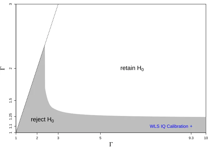
FIGURE 3 : Extended sensitivity curve from the AR study calibrated to the

estimates of ability bias from the WLS study (cross). . . 61

FIGURE 4 : Histogram ofπ∗ estimated for 171 same-sex, full-sibling pairs from the WLS study. . . 63

FIGURE 5 : Stylized plot of data from a comparative interrupted time series

design. . . 73

FIGURE 6 : Age-adjusted firearm homicide rates in Missouri and states

border-ing Missouri (population-weighted averages), 1999-2016. . . 84

FIGURE 7 : Age-adjusted gun homicide rates in Missouri, lower control states,

and upper control states, 1999-2016. . . 86

FIGURE 8 : Histograms of placebo “repeal” effects using upper and control states. 88

FIGURE 9 : Relative trends of homicide rates for Missouri, upper controls, and

lower controls. . . 98

FIGURE 10 : Causal diagrams for MR (left) and MFD (right). . . 106

FIGURE 11 : 2×2 table for Mendelian factorial design. . . 116

FIGURE 12 : Distributions of simulated MFD estimator ˆτ and naive estimator ˆ

τ0 over several settings. . . 127

FIGURE 13 : Comparing densities and means of ˆτ0, ˆτ, and ˆτbnd across 5000

FIGURE 14 : Absolute proportional bias and RMSE for MFD, naive, and bounded

estimators. . . 131

FIGURE 15 : Power against two-sided alternative and coverage for MFD, naive,

CHAPTER 1

Introduction

The objective of many social science, epidemiology, and medical research studies is to

iden-tify and estimate causal relationships between treatments or exposures and outcomes of

interest. In observational studies, the absence of physical randomization and the lack of the

tightly controlled environment of a well planned experiment may lead critical observers to

call causal conclusions into question. Although less of a concern in randomized trials where

treatment is assigned at random, bias may still enter the equation through other means. For

example, outcomes attributable to a disease of interest may be aliased with outcomes caused

by other diseases when the symptoms associated with the disease are unspecific. Resulting

case definitions are usually inexact and can lead to substantial bias even in otherwise well

designed trials. Consequently, in both observational and randomized settings, anticipating

and addressing plausible patterns of unmeasured confounding should be an objective of any

research. In Chapters 2 through 5 we given four examples of how we address this objective

through developments in both statistical design andanalysis.

Chapters 2 and 3 approach the issue of bias in matched-pair studies through analysis,

improving existing sensitivity analysis methods to more effectively address certain plausible

patterns of bias.

In Chapter 2, we introduce a sensitivity analysis framework that allows for the investigator

to interpret the sensitivity parameter as a bound on the average bias present in a

matched-pair study with binary outcomes (Hasegawa and Small, 2017). The new interpretation

resolves difficulties of the standard sensitivity analysis that bounds the maximal bias to

which pairs are subject, when the pattern of bias is presumed to be heterogeneous

(Rosen-baum, 1987). Specifically, when some pairs may suffer from arbitrarily large biases, but on

the average the study is more moderately biased, the average case sensitivity analysis will

of talking on a mobile phone on the incidence of car accidents (Tibshirani and Redelmeier,

1997).

In Chapter 3, we extend this framework using modern convex optimization tools to allow

for continuous outcomes and a simultaneous bound on both the maximal and average (or

typical) bias in a matched pair study. We call this the extended sensitivity analysis

frame-work (Fogarty and Hasegawa, 2019). In addition to bounding sample-level bias, extended

sensitivity analysis lets the investigator place bounds on the typical bias present in a

su-perpopulation from which the paired sample was drawn. This allows for calibration of a

sensitivity analysis in one study to information on confounding from another study whose

sample was generated from the same superpopulation as the first. We apply these new

methods to two sibling studies on the effects of education on future earnings. We calibrate

the extended sensitivity of one study where IQ data was not collected to an estimate of

bias introduced by differences in ability between siblings from the second study where IQ

data was collected. Empirically, the example suggests that ability bias is heterogeneous

across sibling pairs; the bias is typically modest but there is a small proportion of sibling

pairs where the differences in ability are quite large. We demonstrate that the extended

sensitivity analysis is better suited than the standard sensitivity analysis in such settings.

Through design, Chapter 3 addresses bias in comparative interrupted times series when the

parallel trends assumption of the standard difference-in-difference design fails because of an

interaction between history and the groups under comparison (Hasegawa et al., 2019). We

develop a difference-in-difference based design that allows for partial identification of causal

effects when the parallel trends assumption fails. We re-analyze a study of the repeal of

Missouri’s permit-to-purchase law and its effect on firearm homicide rates (Webster et al.,

2014) using our prosed method. The repeal occurred concurrently with the Great Recession

and there is concern that the firearm homicide trends in Missouri and the control states

may have been differentially affected by the onset of recession. Our method provides partial

with the different groups.

Finally, in Chapter 5, we give another example of how improved design can mitigate

con-cerns of bias, this time in a randomized control trial to assess the efficacy of a malaria

vaccine. Symptoms of clinical malaria have significant overlap with the symptoms of other

common childhood illnesses. Furthermore, children in endemic areas are able to tolerate

varying levels of parasitemia without symptoms. Together, these facts make distinguishing

between malaria-attributable symptoms and non-malaria symptoms very challenging.

In-exact case definitions currently in use can substantially bias estimates of vaccine efficacy.

In this chapter, we leverage genetic traits that are protective against malaria but not other

childhood illnesses to identify vaccine efficacy in a randomized control trial. The sickle cell

trait is one such genetic variant that confers protection specifically against clinical malaria.

The method, which we call mendelian factorial design, is inspired by mendelian

random-ization studies that use genetic variants as instrumental variables to estimate causal effects

of non-randomized exposures. Under realistic assumption, this new study design allows for

CHAPTER 2

Sensitivity Analysis for Matched Pair Analysis of Binary Data: From Worst Case to

Average Case Analysis

Abstract

In matched observational studies where treatment assignment is not randomized,

sensitivity analysis helps investigators determine how sensitive their estimated

treat-ment effect is to some unmeasured confounder. The standard approach calibrates the

sensitivity analysis according to the worst case bias in a pair. This approach will result

in a conservative sensitivity analysis if the worst case bias does not hold in every pair.

In this paper, we show that for binary data, the standard approach can be calibrated

in terms of the average bias in a pair rather than worst case bias. When the worst case

bias and average bias differ, the average bias interpretation results in a less conservative

sensitivity analysis and more power. In many studies, the average case calibration may

also carry a more natural interpretation than the worst case calibration and may also

allow researchers to incorporate additional data to establish an empirical basis with

which to calibrate a sensitivity analysis. We illustrate this with a study of the effects of

cellphone use on the incidence of automobile accidents. Finally, we extend the average

case calibration to the sensitivity analysis of confidence intervals for attributable effects.

2.1. Introduction

2.1.1. Sensitivity analysis as causal evidence

In matched-pair observational studies, causal conclusions based on usual inferential methods

(e.g., McNemar’s test for binary data) rest on the assumption that matching on observed

covariates has the same effect as randomization (i.e., that there are no unmeasured

con-founders). In other words, it is assumed that there are no unobserved covariates relevant to

both treatment assignment and outcome. A sensitivity analysis assesses the sensitivity of

results to violations of this assumption. Cornfield et al. (1959) introduced a model for

modern approach to sensitivity analysis is introduced in Rosenbaum (1987); Rosenbaum’s

approach builds on Cornfield’s model (Cornfield et al. (1959)) but incorporates uncertainty

due to sampling variance. There are other contemporary sensitivity analysis models, see

for example McCandless et al. (2007) for a Bayesian approach, but we restrict our focus to

Rosenbaum’s approach. Rosenbaum’s sensitivity analysis yields an upper limit on the

mag-nitude of bias to which the result of the researcher’s test of no treatment effect is insensitive

for a given significance level α. More specifically, Rosenbaum (1987) derives bounds on the p-value of this test given an upper bound, Γ, on the odds ratio of treatment assignment

for a pair of subjects matched on observed covariates. Γ can be thought of as a measure

of “worst case” bias in the sense that treatment assignment probabilities in matched pairs

are allowed to vary arbitrarily as long as the odds ratio of treatment assignment for a pair

of subjects is no greater than Γ. The largest Γ for which the p-value is less than 0.05 is

denoted by Γsens. We will use Γtruthto distinguish the true unknown worst case bias. Γsens

is interpreted in Rosenbaum’s sensitivity analysis as the largest value of the worst case bias

across matched pairs that does not invalidate the finding of evidence for a treatment effect.

We refer to this as aworst case calibrated sensitivity analysis. A classic example of this type

of analysis is given in Chapter 4 of Rosenbaum (2002c). Applying the worst case sensitivity

analysis to a study of the effects of heavy smoking on lung cancer mortality (Hammond

(1964)), Rosenbaum finds that Γsens≈6 and interprets this result cogently:

To attribute the higher rate of death from lung cancer to an unobserved covariate

rather than to an effect of smoking, that unobserved covariate would need to

produce a sixfold increase in the odds of smoking, and it would need to be a

near perfect predictor of lung cancer.

A brief, more formal review of Rosenbaum’s sensitivity analysis framework is in Section

2.2.2.

The worst case calibrated sensitivity analysis raises several potential questions. If we are

six times as likely to smoke as the other (i.e., Γtruth≤Γsens), then we would conclude that

our study provides convincing evidence that heavy smoking increases the rate of lung cancer

mortality. However, what if, on average, unmeasured confounders do not alter the odds of

smoking greatly but there are some subjects for whom the unmeasured confounders make

them almost certain to smoke, e.g., a subject who experiences huge peer pressure to smoke.

If such a subject ends up in our sample of matched pairs, and we condition on matched pairs

in which only one unit receives treatment, a standard practice when conducting matched

pair randomization tests, then the odds ratio of treatment assignment in the matched pair

containing that subject, and consequently Γtruth, will be infinite. In such a case, since

Γsens is generally finite, we’d expect it to be smaller than Γtruth. Now, suppose that there

are such pairs in the Hammond study but that for most pairs the odds ratio of smoking

between the units is much smaller than six. Using the worst case calibrated sensitivity

analysis, we would conclude that the study is sensitive to bias. Is there potentially some

natural quantification of average bias over the sample of matched pairs, say, Γ0_truth, that isn’t infinite and perhaps is smaller than six? And if we calibrate our sensitivity analysis to

this measure of bias rather than the worst case measure, will the sensitivity analysis be valid

in the sense that the inference is conservative at level α for any Γ ≥Γ0_truth? If it is valid, are there other advantages to using theaverage case calibrated sensitivity analysis over the

worst case calibrated sensitivity analysis? In what follows, we attempt to answer these

motivating questions in the context of a matched pair analysis of the association between

cellphone use and car accidents.

2.1.2. Outline

In this paper we demonstrate that interpreting sensitivity analysis results in terms of average

case rather than worst case hidden bias is both valid and conceptually more natural in many

common scenarios. To illustrate our claim that the average case analysis is more natural

we will perform a causal analysis of a study by Tibshirani and Redelmeier (1997) that asks

described in the following section. In section 2.2 we review the model for sensitivity analysis

of tests of no treatment effect and sensitivity intervals for attributable effects for binary data.

In section 2.3 we discuss the theory behind the validity of average case sensitivity analysis.

Finally, the Tibshirani and Redelmeier (1997) study is examined in this new light in section

2.4. In particular, we see how the average case sensitivity analysis makes it possible to use

additional information from the problem to empirically calibrate our sensitivity analysis in

Section 2.4.1 and we extend the average case sensitivity analysis to the study of sensitivity

intervals for attributable effects in Section 2.4.3.

2.1.3. Motivating Example: Effects of cellphone use on the incidence of motor-vehicle

col-lisions

Tibshirani and Redelmeier (1997) conducted a case-crossover study of the effects of cellphone

use on the incidence of car collisions. In a case-crossover study each subject acts as her own

control which has the benefit of controlling for potential confounders that are time-invariant,

even if they are unobserved. Data collection took place at a collision reporting center in

Toronto between July 1, 1994 and August 31, 1995 during weekday peak hours (10 AM to 6

PM). Consenting drivers who reported having been in a collision with substantial property

damage and who owned a cellphone were included in the study. Drivers involved in collisions

that involved injury, criminal activity, or transport of dangerous goods were excluded. The

resulting study population included 699 individuals who gave permission to review their

cellphone records and filled out a brief questionnaire about their personal characteristics

and the features of the collision. The matched pair analysis compared cellphone usage in

the 10-minute hazard window prior to the crash with a 10-minute control window on a

chosen day prior to the crash. We will denote the time of the crash as t and the hazard window ast−10 tot−1 minutes. The authors examined several different control windows:

1. Previous day: timet−10 to t−1 minutes on the previous day.

crash took place on a weekday and similarly if the crash took place on a weekend.

3. One week prior: timet−10 to t−1 minutes one week prior to the collision.

4. Busiest cellphone day of previous three days: time t−10 to t−1 minutes on the one day among the prior three to the collision with the most cellphone calls.

For each choice of control window, Tibshirani and Redelmeier (1997) found that there was

a significant positive association between cellphone usage and traffic collision incidence.

The 2 x 2 contingency tables shown in Table 1 summarize the data using the four different

control windows.

Control

On phone Not on phone Previous Weekday/end

Hazard On phone 12 158

Not on phone 23 506 One Week Prior

Hazard On phone 6 164

Not on phone 21 508 Previous Driving Day

Hazard On phone 18 119

Not on phone 20 171 Most Active Cellphone Day

Hazard On phone 17 135

Not on phone 43 504

Table 1: One Week Prior: results for one week prior control window versus hazard window;Previous Weekday/end: results for previous weekday/weekend control window versus hazard window; Previous Driving Day: results for previous driving day control window versus hazard window;Most Active Cellphone Day: results for most active cellphone day in previous 3 days control window versus hazard window.

2.1.4. Sensitivity of results to hidden bias

As this was an observational study, the associations cannot be assumed to be causal. We

would like to quantify how large a hidden bias would have to be to explain the observed

analysis seems appropriate and is a straightforward exercise (see Chapter 4, Rosenbaum

(2002c) for example). Table 2 shows the results of a standard worst case sensitivity analysis

for each control window. Here, Γsens is the largest value of Γ such that the result are still

significant at theα= 0.05 level. In our analysis of the case-crossover study from Tibshirani and Redelmeier (1997) we condition on subjects who were on a cellphone in exactly one of

the control and hazard windows (i.e., discordant case-crossover pairs). Thus, the odds ratio

of treatment assignment for the two windows observed for any case-crossover subject can

be viewed as the conditional odds that treatment occurs in a particular window. Hence,

we can interpret Γ as the maximum (and 1/Γ as the minimum) over all study subjects of the odds that a driver is using a cellphone during the hazard window and not during the

control window.

Control Window Γsens

previous weekday/weekend 4.92 one week prior 5.53 previous driving day 4.15 most active cellphone day 2.40

Table 2: Sensitivity analysis for (marginal) α= 0.05.

The sensitivity analysis suggests that the most active cellphone day control window was the

most conservative analysis. This is unsurprising since we would expect that the treatment

assignment (cellphone use) would be biased toward the control window on a day when you

used a cellphone relatively often. We can interpret these results as follows: the observed

ostensible effect is insensitive to hidden bias that increases the odds that a driver was on

a cellphone in the hazard window and not the control window on the most active cellphone

day by at most a factor of 2.4. In many observational studies this type of statement is

very useful. However, it may be plausible that some study participants are exposed to

infinite (or at least very large) hidden bias. For example, this happens if a subject was not

driving during the control window and (almost) always uses her landline rather than her

treatment is received in exactly one of the windows – a standard practice when conducting a

matched pair randomization test – such a driver is always on a cellphone during the hazard

window. When this happens, the observed ostensible effect is (almost) always sensitive to

hidden bias, no matter how strong the observed association. Implicitly, in the worst case

sensitivity analysis, the investigator is supremely skeptical; she assumes that it could be that

all study participants suffer from the worst case hidden bias which, when it is possible that

some study participant suffers from unbounded hidden bias, renders sensitivity analysis

under the standard worst case interpretation uninformative. Yet in many studies where

unbounded hidden bias in some matched pairs is plausible, as in our motivating example,

we still want to examine the sensitivity of our results to potential hidden bias. If we

could perform a valid, average case calibrated sensitivity analysis then we could (1) make

sensitivity analysis informative even in the presence of pairs subject to unbounded hidden

bias and (2) make the interpretation of sensitivity analysis results far less conservative. It

turns out that there is a measure of the sample average bias that is generally finite in the

presence of pairs subject to unbounded bias for data with binary treatment and outcome.

Moreover, the sensitivity analysis calibrated to this measure of average bias is valid when

using McNemar’s statistic to test the null hypothesis of no treatment effect against the

alternative of a positive treatment effect (i.e., that talking on a cellphone while driving

increases the rate of automobile accidents).

2.2. Notation and Review

2.2.1. Notation

Our study sample consists ofSmatched pairs where each pairs= 1,2, . . . , Sis matched on a set of observed relevant covariatesxs1 =xs2 =xs. Units in each pair are indexed byi= 1,2.

We let Zsi and Rsi denote the treatment assignment and outcome, respectively, of thei-th

unit of the s-th pair. The potential outcomes under treatment and control are denoted as rT si and rCsi, respectively. Hence, we can write Rsi = ZsirT si + (1−Zsi)rCsi. Under

Rsi =rCsi. Hereafter, we will work under the null hypothesis and under the assumption that

each pair was matched on some set of observed covariatesxs. Additionally, we assume that

there is some unobserved covariateUsi that is associated with both treatment assignment

and outcome and letusibe the realization ofUsifor thei-th unit of thes-th pair. Within pair

differences in treatment and outcome will be denoted asVs=Zs1−Zs2andys=rCs1−rCs2.

It will be convenient to define the following vector quantities: Z = (Z11, Z12, . . . , ZS2)T,

r= (rC11, rC12, . . . , rCS2)T,U= (U11, U12, . . . , US2)T, and A= (|y1|,|y2|, . . . ,|yS|)T.

To be very clear about the information on which we are conditioning we will define some

important information sets. Let F ={(xs, usi, rCsi, rT si) : s= 1,2. . . , S, i= 1,2} be the

set of fixed observed and unobserved covariates for all units. Let Z = {Z: |Vs|= 1, s=

1, . . . , S}be the set of matched pairs such that only one unit receives treatment. We assume that Ris binary and we define A1 ={A: |ys|= 1, s= 1, . . . , S}. So Z ∩ A1 is the set of

discordant matched pairs. In the analysis that follows, we will condition on F,Z ∩ A1.

2.2.2. Review: sensitivity analysis for binary data

Under the assumption that all variables that confound treatment assignment are observed,

Zsi⊥⊥(rCsi, rT si)|Xs (Ignorability)

our matched observational study should closely resemble a randomized study and thus

P(Z=z| F,Z ∩ A1) = 1/2S forz∈ Z. In practice, this assumption is rarely valid and the

probability of treatment assignment depends materially on the unobserved covariates U.

A second assumption made in the causal framework introduced in Rosenbaum and Rubin

(1983) is the Positivity assumption – 0 < P(Zsi = 1|Xs) < 1 for all s = 1,2, . . . , S and

i = 1,2 – which says that all units have a chance of receiving treatment. In our case-crossover study, however, this may not be an appropriate assumption. We introduce an

example of how our case-crossover study might violate the positivity assumption in Section

of positivity.

When bothZandrare binary it is common to use McNemar’s statistic to test for treatment effect:

Definition 1. For a matched pair study with binary treatment and outcome we define

McNemar’s statistic to be

T(Z,r) =

S X

s=1

1{VsYs = 1}. (2.1)

Under the null distribution of no treatment effect T(Z,r) follows a Poisson-Binomial dis-tribution with probabilities {p1, p2, . . . , pS} whereps=P((Zs1−Zs2)(rs1−rs2) = 1) is the

probability that the unit with positive outcome, i.e., r= 1, receives treatment in pair s. If we consider only discordant pairs and we assume, without loss of generality, that the first

unit in each pair is the unit with positive outcome we may write

ps=P(Zs1 = 1|F,Z ∩ A1). (2.2)

Recall that the Poisson-Binomial distribution is the sum of independent, not necessarily

identical Bernoulli trials. If Xs contains the complete set of relevant covariates then ps

equals 1/2 for all pairs and we can conduct inference using B(1/2, S) as our null distri-bution, effectively treating our data as being the outcome of a randomized study. As we

mentioned earlier in this section, if there is some unobserved characteristicU that is relevant to treatment assignment and outcome then{p1, . . . , pS}are unknown and consequently the

exact null distribution is no longer available to the investigator. When this is the case,

a sensitivity analysis like the one conducted informally in Section 2.1.4 can be used to

determine how sensitive the investigator’s conclusions are to departures from the ideal

ran-domized design. Following Chapter 4 of Rosenbaum (2002c) we can formalize the notion of

where

1

1 + Γ ≤P(Zs1= 1|F,Z ∩ A1)≤ Γ

1 + Γ (2.3)

for all s = 1, . . . , S and where Γ ≥ 1 is the sensitivity parameter that bounds the extent of departure from a randomized study. Proposition 12 in Chapter 4 of Rosenbaum (2002c)

states that (2.3) is equivalent to the existence of the following model

log

ps

1−ps

=γ(us1−us2) , s= 1, . . . , S (2.4)

where exp(γ) = Γ, γ ≥ 0, and usi ∈[0,1] for s= 1, . . . , S and i= 1,2. The restriction of

the unobserved confounder to the unit interval in this equivalent representation preserves

the non-technical interpretation of Γ used in section 2.1.4 as a bound on the odds that the

driver was talking on a cellphone in the hazard window. Henceforth, we assume that Usi

and its realization usi belongs to the unit interval fors = 1, . . . , S and i= 1,2. However,

the distribution ofUsi on the unit interval may be arbitrary.

Under this sensitivity model, if we letT+be binomial with success probability Γ/(1+Γ) and

T−be binomial with success probability 1/(1 + Γ) it follows from Theorem 2 of Rosenbaum (1987) that

P T−≥k≤P(T ≥k|F,Z ∩ A1)≤P T+≥k (2.5)

for allk= 1, . . . , S. This inequality is tight in the sense that it holds for any realizationuof

U. For conducting a hypothesis test, the stochastic ordering in (2.5) gives us bounds on the

p-value of our test for a given magnitude of bias Γ. If Γ ≥Γtruth, then T+ yields a valid,

albeit conservative, reference distribution for testing the null hypothesis of no treatment

effect against the alternative of a positive treatment effect.

2.2.3. Attributable effects for binary outcomes: hypothesis tests and confidence intervals

Attributable effects are a way to measure the magnitude of a treatment effect on a binary

treated subjects that would not have occurred if the subject was not exposed to treatment.

In this section, we review Rosenbaum (2002a)’s procedure to construct one-sided confidence

statements about attributable effects in the context of the cellphone case-crossover study.

LetSebe the number of all pairs in the study, discordant or not, and let the first S be the

discordant pairs. If we assume thatrT si ≥rCsi, that talking on a cellphone cannot prevent

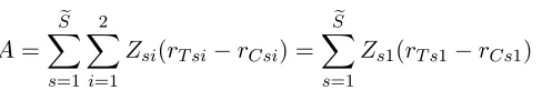
an accident, then we can write the attributed effect as

A= e

S X

s=1 2 X

i=1

Zsi(rT si−rCsi) =

e

S X

s=1

Zs1(rT s1−rCs1) (2.6)

where the first unit of s-th pair is the observation from the hazard window. Why does the second equality hold? If the subject was talking on a cellphone in the control window, that

is Zs2 = 1, then we observerT s2 = 0 which by our assumption that talking on a cellphone

cannot prevent an accident implies that rCs2 = 0. So attributable effects can only occur

among discordant pairs where the subject was talking on a cellphone in the hazard window

or concordant pairs where the subject was talking on a cellphone in both windows. The

following table characterizes the four types of possible pairs in our case-crossover study,

Zs1 Zs2 Rs1 Rs2 rT s1 rCs1

D(+,−) 1 0 1 0 1

-D(−,+) 0 1 1 0 1 1

C(−,−) 0 0 1 0 1 1

C(+,+) 1 1 1 0 1

-Table 3: The four possible types of pairs in our case-crossover study. D and C indicate discordant and concordant pairs, respectively, and the + and−indicate if a unit in the pair was treated or not, respectively.

D and C indicate discordant and concordant pairs, respectively. D(+,−) is the set of discordant pairs where the subject was on a cellphone in the hazard window, D(−,+) is the set of discordant pairs where the subject was on a cellphone in the control window,

on a cellphone in either window. If there are no attributable effects then we know that

rCs1 = 1 in D(+,−) and C(+,+) and we have that Rs1 =rCs1 for all pairs s, concordant

or discordant. We can write the probability that the subject was talking on a cellphone at

the time of accident for each type of pair as (1) P(Zs1Rs1= 1|D(+,−)∪D(−,+)) = ps,

wherepshere is equivalent to theps defined in Section 2.2.2 when there are no attributable

effects; (2) P(Zs1Rs1= 1|C(−,−)) = 0; and (3) P(Zs1Rs1 = 1|C(+,+)) = 1. Now let

c+_{=|C(+,+)|denote the cardinality of the set of concordant pairs where the subject was}

on a cellphone in both windows and let s = S + 1, . . . , S +c+ be the pairs belonging to

C(+,+). Then if A= 0 we can define the standardized deviate for McNemar’s statistic T

as

e

T =

PS

s=1Zs1rCs1−PSs=1ps n

PS

s=1ps(1−ps)

o1/2

=

PS+c+

s=1 Zs1Rs1−

PS

s=1ps+c+

n

PS

s=1ps(1−ps)

o1/2 . (2.7)

e

T defines a normal reference distribution for PS

s=1Zs1rCs1 that we can use to conduct

approximate inference. If A = a > 0, then Z

e

s1Res1 = Zes1rTse1 = Zes1(rCes1+ 1) for pair se belonging to the set of a pairs with attributable accidents and the second equality above does not hold. When this equality fails to hold, the standard normal deviate Te cannot

be computed from the observed data conditional on F. How then can we adjust Te for

attributable accidents so that it can be computed from the observed data? Because we’ve

assumed talking on a cellphone cannot prevent an accident, we only need to consider two

cases. If pairs_ebelongs toD(+,−) then we subtractZ

e

s1(rTes1−rCes1) = 1 from

PSe

s=1Zs1Rs1,

p

e

s from the expectation, andpes(1−pse) from the variance term. Ifesbelongs toC(+,+) we again subtract 1 from PSe

s=1Zs1Rs1 and subtract 1 from the |C(+,+)| in the expectation

while leaving the variance term unchanged.

ifδsj = 0 whenever Zsj = 1 and Rsj = 0 or Zsj = 0 and Rsj = 1. Under this definition, we

can express the number of attributable effects as A =ZTδ. For a compatible δ such that

ZTδ=awe denoteTe_−δ to be Teadjusted for the a attributable effects. Te_−δ defines a new

reference distribution for PS

s=1Zs1rCs1 under the null hypothesis that potential accidents

indicated byδ are attributable to talking on a cellphone while driving. We can write Te_−δ

as

e

T−δ=

PS+c+

s=1 Zs1Rs1(1−δs1)−

PS

s=1(1−δs1)ps+

PS+c+

s=S+1(1−δs1)

n

PS

s=1(1−δs1)ps(1−ps)

o1/2 . (2.8)

Using the notion of asymptotic separability (Gastwirth et al. (2000)), Rosenbaum (2002a)

show that choosing a compatibleδ∗ ≡δ∗(a) withZTδ∗(a) =athat maximizes the expecta-tion, and when there are ties to maximize the variance term, yields a reference distribution

that, asymptotically, has the largest upper tail area among compatibleδ(a). Thus, we can use T−δ∗ to test the plausibility that there are at most aattributable effects. Since A is a

random variable we refrain from calling this a hypothesis test, a term usually reserved for

unknown parameters. From equation (2.8) we see thatδ∗(a) includes theapairs inD(+,−) with the smallest values of ps.

It is possible to invert the one-sided “plausibility tests” introduced above using T−δ∗ that

we just introduced in order to construct a confidence interval for attributable effects of the

form {A : A > a}. It turns out that if it is plausible that there are aattributable effects then it is also plausible that there area+ 1 attributable effects (Rosenbaum (2002c)). This monotonicity property leads to a very simple procedure to construct a one-sided confidence

interval in the absence of hidden bias. First, ifps = 1/2 for all s= 1,2, . . . ,Sethen for any

a≥0 we can compute Te_−δ∗ ={T −a−(S−a)/2}/{(S−a)1/2/2}.

Next, starting with a = 0 we check if Te−δ∗ < Φ−1(1−α), incrementing a by one if it

isn’t and stopping if it is. Finally, let a∗ be equal to one less the value of a at which we terminate the procedure. Using the monotonicity result above we have that{A : A > a∗}

If we bound the worst case calibrated bias above by Γ then we can construct a one-sided

100×(1−α)% confidence interval following the same procedure but instead usingTe−δ∗_,Γ= {T−a−(S−a)pγ}/{(S−a)pγ(1−pγ)}1/2as our standard deviate wherepγ= Γ/(1+Γ). The

resulting one-sided 100×(1−α)% confidence interval is referred to as a sensitivity interval (See Chapter 4, Rosenbaum (2002c)). For a detailed illustration of these procedures we

refer the reader to Sections 3-6 of Rosenbaum (2002a).

2.3. From Worst Case to Average Case Sensitivity Analysis

2.3.1. Valid average case analysis: binary outcome

An investigator conducting a sensitivity analysis tries to determine a test statistic whose

null distribution is known conditional on the presence of hypothetical bias Γ. Since the

distribution of Usi is unknown, traditionally, the investigator assumes the worst. That is,

the null distribution is constructed assuming that in each pair us1 = 1 and us2 = 0. As

noted in Section 2.2.2, T+ yields a valid reference distribution for testing the null of no-treatment effect when Γ≥Γtruth. However, such a test is inherently conservative because it

is designed to be valid for any realization ofU sinceUand thus sincep= (p1, . . . , pS)T are

generally unknown. This is why we resort to a sensitivity analysis where we allowpsto vary

arbitrarily as long as ps/(1−ps) ≤Γ. In Section 2.1.1 we asked whether there was some

natural quantification of average bias to which we could calibrate our sensitivity analysis

which would lead to a less conservative analysis than the worst case calibration. One such

quantification is Γ0_truth=p/(1−p) wherepis the sample average ofps. In what follows, we

show that if we calibrate our sensitivity analysis to Γ0_truthit will be valid and less conservative than the worst case calibration. To prove this, we show thatT0 ∼B(Γ0_truth/(1 + Γ0_truth), S) yields a valid reference distribution for testing the null of no treatment effect against the

alternative of a positive treatment effect. In Theorem (2) below, we prove that the upper

tail probability for McNemar’s statistic T is bounded above by the upper tail probability forT0.

Theorem 2. Set p=

PS

s=1ps

/S andΓ0_truth =p/(1−p) and letVs

iid

Γ0_truth))for all s= 1,2, . . . , S. Define T0=V1+· · ·+VS. Then

Pr(T ≥a|F,Z ∩ A1)≤Pr T0≥a

for all a≥Sp.

Proof. Observe that p majorizes p·1 and note that if a function f(p) is Schur-convex in

p then f(p) ≥ f(p1). What remains to be shown is that the distribution function for a Poisson-Binomial is Schur-convex in p. See Gleser (1975) for this approach and Hoeffding

(1956) for the original proof. The theorem as stated is an immediate corollary of Theorem

4 in Hoeffding (1956). Gleser (1975) presents a more general version of this result which

holds when the success probabilities of T majorize those ofT0.

Remark 1. Theorem (2) is a finite sample result whose proofs we refer to are both rather

technical. An analogous asymptotic result follows from much simpler arguments. The

vari-ance of a Bernoulli random variable with success p can be written as f(p) =p(1−p). f is clearly concave and thus by Jensen’s Inequality, Var(T) ≤ Var(T0). Since the expectation of T and T0 are equal, using a normal approximation to the exact permutation test will asymptotically yield the same stochastic ordering as in Theorem (2).

Remark 2. It is important to note that Γ0_truth ≤ Γtruth since ps/(1−ps) ≤ Γtruth for

s = 1, . . . , S. Consequently, we have that Pr(T0≥a) ≤ Pr(T+ _{≥a) which implies that}

sensitivity analysis with respect to Γ0, the average case calibrated sensitivity analysis, is less conservative than the worst case calibrated sensitivity analysis with respect to Γ.

The implication of this theorem is that it is safe to interpret a sensitivity analysis in terms

of Γ0, an upper bound on the sample average hidden bias (p/(1−p)). For example, when using the most active cellphone day control window we have Γsens = 2.4. Previously, we

would say that if no case-crossover pair was subject to hidden bias larger than 2.4, then the

data would still provide evidence that talking on a cellphone increases the risk of getting in

a car accident. Now, some case-crossover pairs may be subject to hidden bias (much) larger

than 2.4, as long as the sample average hidden bias is no larger than 2.4. It is important to

Schur-convexity of the distribution function of our test statistic with respect to p which requires

that it be symmetric inp. For more general tests, such as the sign-rank test, this is not the

case.

Some additional applications of Theorem 2 can be found in the Appendices. Appendix A

considers the case whenUs1 and Us1 measure some time-varying propensity of subject sto

use his cellphone. Using Theorem 2 we develop a little theory and a numerical example.

Appendix B provides details on how Theorem 2 can be applied when U is not restricted to the unit interval.

2.4. The Effect of Cellphone Use on Motor-vehicle Collisions

In this section we return to our motivating example to see how our average case theory can

provide interpretive assistance to our standard sensitivity analysis we carried out in Section

2.1.4 and allow us to incorporate additional information to empirically calibrate our average

case sensitivity analysis.

2.4.1. Driving intermittency

The study conducted in Tibshirani and Redelmeier (1997) did not have access to direct

information on whether an individual was driving during the control window. The authors

examine the effect of driving intermittency during the control window on their relative-risk

estimate by bootstrapping the estimate using an intermittency rate of ρb= 0.65. In other

words, they correct for bias due to the possibility that a subject was not driving during the

control window. The intermittency rate was estimated using a survey asking 100 people

who reported car crashes whether they were driving at the same time the previous day.

Alternatively, one may ask a related question in the context of a sensitivity analysis - does

the bias due to driving intermittency explain the observed association between cellphone

usage and traffic incidents? Given that the study took place in the early 1990s when, for

some cellphones and carphones were synonymous, it would not be surprising if many study

driving, violating the positivity assumption. Therefore, the only plausible Γtruth is infinite

(or at least very large) when conditioning on case-crossover pairs where the subject is on her

cellphone in only one of the two windows. This renders the worst case sensitivity analysis

uninformative. No magnitude of association between cellphone use and car accidents would

convince us that the relationship was causal if we stuck to the worst case calibration of the

sensitivity analysis. The average case calibration, on the other hand, still has a chance. We

can use our estimateρ_bto approximate a plausible value ofp,p= (1−ρ_b)·1 +ρ_b·0.5 = 0.675, and a corresponding plausible value of Γ0_truth, Γ0_truth = p/(1−p) = 2.1. Theorem (2) circumvents the conceptual hurdle of unbounded Γtruth and allows us to confidently use a

sensitivity analysis to quantitatively assess the causal evidence. Moreover, it allows us to

incorporate information aboutρ into our analysis. If the association between cellphone use and motor vehicle collisions is causal in nature, our empirical calibration suggests that our

test for treatment effect should be insensitive to unobserved biases with magnitude Γ0≈2.1.

2.4.2. An alternative approach to handling pairs with unbounded bias

There are other approaches to dealing with the example of infinite bias we just presented.

For instance, the investigator may be more confident in specifying an upper bound on the

worst case bias to be finite, Γ<∞, for a proportion 1−β of the matched pair sample than he is in working in terms of the average case bias. If he has a good sense of what proportion

β of the pairs is exposed to unbounded bias he may drop β×S pairs where the treated unit had positive outcome and perform the standard worst case sensitivity analysis on the

remaining (1−β)×S pairs. Rosenbaum (1987) proved that this method yields a valid sensitivity analysis. This strategy would be particularly suited for the example of driver

intermittency discussed above. However, this approach assumes this particular pattern of

unmeasured confounding is present and driver intermittency is just one of many sources of

potential bias. On the other hand, the average case analysis accomodates arbitrary patterns

2.4.3. Average case sensitivity analysis for attributable effects

How many of the recorded accidents in our study can be attributed to the driver talking on

a cellphone? Recall from Section 2.2.3 that the set indicated by δ∗ includes the apairs in

D(+,−) with the smallest values ofps. Although we cannot computeTe−δ∗ and thus cannot

use it directly to conduct inference, we can compute a lower bound that we will show can

be used to perform an average case sensitivity analysis:

e

T−δ∗ =

PS

s=1Zs1rCs1−PsS=1(1−δs∗1)ps n

PS

s=1(1−δ∗s1)ps(1−ps) o1/2

=

PS

s=1Zs1Rs1(1−δ

∗

s1)−

PS

s=1(1−δ

∗

s1)ps n

PS

s=1(1−δ∗s1)ps(1−ps) o1/2

= T −a−(S−a)p(a)

n

PS

s=1(1−δ∗s1)ps(1−ps) o1/2

≥ T −a−(S−a)p(a)

{(S−a)p(a)(1−p(a))}1/2 =Te(p(a)) (2.9)

wherep(a) =PS

s=1(1−δs∗1)ps/(S−a). The last inequality follows from Jensen’s inequality

applied to the variance term in the denominator. Notice that instead of applying Theorem

(2) in order to derive a sensitivity analysis in terms of the average bias we use the simpler

argument in Remark (1). Now note that if ps ≥p∗ for all s= 1, . . . , S then we can relate

the trimmed average probability,p(a), top as follows

p≥ (S−a)p(a) +a·∗

S =q(a). (2.10)

We can use this relationship to construct a simple procedure – mirroring that of Section

2.2.3 – to perform an average case calibrated sensitivity analysis for one-sided confidence

1. Choose a desired average calibrated sensitivity parameter Γ0.

2. For a= 0 solve q(a) = Γ0/(1 + Γ0) forp(a) and denote the solution p(a, γ0). Compute

e

T(p(a, γ0)).

3. IfTe(p(a, γ0))<Φ−1(1−α) then conclude it is plausible that none of the accidents can

be attributed to talking on a cellphone.

4. Else, repeat steps (2) and (3) fora= 1, . . . , S stopping when Te(p(a, γ0))<Φ−1(1−α).

Leta∗ =a−1.

5. Return the 100×(1−α)% sensitivity interval {A : A > a∗} and conclude that it is plausible that more thana∗ of the accidents are attributable to talking on a cellphone when exposed to an average bias of at most Γ0.

Just as in the simple test for no treatment effect, we see that we have a nearly identical

procedure to the worst case sensitivity analysis with an average interpretation of the bias

parameter. In fact, the procedure also yields a corresponding worst case calibration for

the computed sensitivity interval. Under the worst case calibration, the sensitivity interval

from step (5) would correspond to a worst case bias Γ =p(a∗, γ0)/(1−p(a∗, γ0)).

How might we apply this procedure to our example? For a given control window we would

like to make confidence statements such as,at the 95% level it is plausible that there are a∗

or more accidents attributable to talking on a cellphone. Recall the empirically calibrated

average case bias from Section 2.4.1, Γ0 ≈2.1. We may also be interested making sensitivity statements such as, if the average probability of talking on a cellphone during the hazard

window is at most 2.1 times that of talking on a cellphone in the control window for drivers

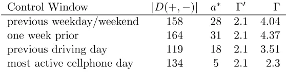
in our study, Γ0 = 2.1, it is plausible at the 95% level that there are a∗ or more accidents attributable to talking on a cellphone. Table 4 summarizes the plausible range of attributable

accidents for each of the four different control windows. For all four control windows we

a cellphone during the control window. The second column reports the lower bound a∗ of the one-sided sensitivity intervals forα= 0.05 We also report the corresponding worst case calibrated bias in the last column of Table 4. In the cellphone study we have no convincing

reason to believe thatp∗>0 but in other examples, it may make sense thatps is bounded

from below, which has the effect of making the procedure less conservative.

Control Window |D(+,−)| a∗ Γ0 Γ previous weekday/weekend 158 28 2.1 4.04 one week prior 164 31 2.1 4.37 previous driving day 119 18 2.1 3.51 most active cellphone day 134 5 2.1 2.3

Table 4: Sensitivity analysis for 95% one-sided confidence intervals for attributable effects of the form {A: A > a∗}. Γ0 indicates the average calibration bias that we specify for the procedure and Γ is the implied worst case calibration that corresponds to the computed interval. We assume that p∗ = 0 .

We find that even if the average probability of talking on a cellphone during the hazard

window was at most 2.1 times that of talking on a cellphone on the same day one week prior,

it is plausible that there are 31 or more accidents attributable to talking on a cellphone. The

implied worst case bias associated with this statement is Γ = 4.37. What this means is that we would arrive at the same conclusion about the number of plausible attributable accidents

if we put an upper bound on the worst case bias of Γ = 4.37 and followed the standard confidence interval procedure for attributable effects outlined in Section 2.2.3 and Gastwirth

et al. (2000). Unlike the sensitivity analysis for the simple test for no treatment effect, the

average case calibrated sensitivity analysis for attributable effects is not guaranteed to be less

conservative than the worst case calibration. For a 95% sensitivity interval for attributable

effects generated by our procedure where a∗ > 0, the corresponding upper bound on the average case bias Γ0 is less than the corresponding upper bound on the worst case bias Γ. This occurs since we do not know which pairs contain attributable effects nor do we know

each pair’s particular exposure to hidden bias. Without any further assumptions, the best

small probability of being on a cellphone in the hazard window and not the control window.

This is expressed mathematically in equation (2.10) by setting p∗ = 0. If Γ0_truth < Γtruth

– which is a reasonable assumption in most circumstances – then using the average case

calibration may still result in a less conservative analysis. However, if all case-crossover pairs

are exposed to the same magnitude of bias such that Γ0_truth = Γtruththen we are guaranteed

to be less conservative by using the worst case calibration. A reasonable solution would be

to simply supply both the Γ0 and Γ when reporting a sensitivity interval, as we do in Table 4. The investigator may then present an argument based on subject matter expertise as to

which calibration is likely to be less conservative.

2.5. Discussion

The theorem presented in 2.3.1 can be thought of as an interpretive aid: For the same

standard sensitivity analysis we now have an additional, often more natural, way to interpret

the results. This new average case interpretation may also allow researchers to make use of

additional information about the problem to empirically calibrate their sensitivity analysis.

As we saw in Section 2.4.1, we used the estimate of driver intermittency rate to determine

an approximate lower bound on Γ0_truth, providing us with some empirical guidance when conducting our sensitivity analysis. In the worst case setting, such an empirical calibration

would not be possible. The investigator performs a sensitivity analysis in anticipation

of critics who might claim the association is due to some unobserved confounder. The

average case analysis makes the protection that the sensitivity analysis provides against such

criticism more robust. As the title of the article makes clear, the results we present are for

binary data. As we illustrated in Section 2.4.3, the notion of attributable effects allows us to

construct interpretable confidence intervals for binary outcomes. We show that our average

case calibration can be extended to the sensitivity analysis of such confidence intervals and

in most cases will yield a less conservative conclusions. It may then be interesting to apply

the results here to the sensitivity analysis of displacement effects, the continuous analog of

effects can be analyzed in the attributable effect framework for binary response, providing

a potential avenue to extend average case calibrated sensitivity analysis to a study with

non-binary outcomes.

2.6. Appendix

2.6.1. Appendix A

Time-varying propensity for cellphone use

After conditioning on the time-invariant driver characteristics X, it may be natural to

modelUsi as a time-varying propensity quantile for using a cellphone in the hazard window

(i = 1) and in the control window (i = 2). Usi could summarize an arbitrary number of

confounding variables that vary between control and hazard windows for driver s. As a quantile, we can think of Usi as coming from a uniform distribution on [0,1]. Us1 and Us2

can conceivably be considered independent since by design a case-crossover study controls

for all individual, time-invariant confounders. Now, suppose that we conduct a sensitivity

analysis that returns Γsens. If we interpret this as an average case hidden bias we may

want to ask how large we would expect the corresponding worst case hidden bias to be.

If we assume the the Usi are propensity quantiles that are iid uniformly distributed we

can compute a lower bound for the expected worst case hidden bias corresponding to the

average case calibrated Γsens. Let Σ be the set of all permutations of {11,12, . . . , S1, S2}

and letσ ∈Σ be an element in the set. Now define γ∗(U) to be the solution to

Γsens/(1 + Γsens) = sup σ∈Σ

(

1

S

S X

s=1

exp(γ(U_σ(s1)−U_σ(s2))) 1 + exp(γ(U_σ(s1)−U_σ(s2)))

)

. (2.11)

The right hand side of this equation inside the supremum operator is an expression for ¯p

under the sensitivity model defined in Section 2.2. The following proposition and corollary

Proposition 1. With probability oneγ∗(U)is the unique solution of (2.11)and the smallest

γ that satisfies

Γsens/(1 + Γsens) =

1

S

S X

s=1

exp(γ(Uσ(s1)−Uσ(s2)))

1 + exp(γ(Uσ(s1)−Uσ(s2)))

for some σ∈Σ.

Proof. It suffices to show that the right hand side of (2.11) is strictly increasing in γ with probability one. Consider 0≤γ1< γ2 and letσ1 be the permutation that maximizes

f(σ, γ1,U) =

1

S

S X

s=1

exp(γ1(Uσ(s1)−Uσ(s2)))

1 + exp(γ1(Uσ(s1)−Uσ(s2)))

.

Assuming that the Usi are iid uniform, U is nonconstant with probability one. If U is

nonconstant then f(σ1, γ1,U) < f(σ1, γ2,U) since Uσ(s1) −Uσ(s2) > 0 for at least one

s= 1, . . . , S. If we letσ2 be the permutation that maximizes f(σ, γ2,U) then we have that

f(σ1, γ1,U)< f(σ2, γ2,U), completing the proof.

Corollary 3. Under the sensitivity model defined in Section 2.2, Γ∗ = exp(γ∗(U)) is a lower bound for the worst case calibrated hidden bias corresponding to the average case

calibrated Γsens givenU.

Using Corollary 3 we can determine the expected lower bound on the worst case hidden

bias corresponding to the average case calibrated Γsens by computing E[Γ∗] via Monte Carlo estimation. The expectation here is taken overU∼ U[0,1]2S. Under this propensity quantile model for the unobserved confounders, this procedure can give us a sense of how

much less conservative the average case calibration is than the worst case calibration. In

the table below we give Monte Carlo estimates and standard errors forE[Γ∗] corresponding to the average case calibrated Γsens for each of the four control windows.

For each control window we find that the average case interpretation is significantly less

Control Window Γsens E[Γ∗] previous weekday/weekend 4.92 24.76 (0.08) one week prior 5.53 31.42 (0.11) previous driving day 4.15 17.66 (0.06) most active telephone day 2.40 5.81 (0.01)

Table 5: Sensitivity analysis for (marginal) α = 0.05 and the expected lower bound on corresponding worst case calibrated biasE[Γ∗]. Standard errors for Monte Carlo estimates are in parentheses.

sensitivity analysis we can conclude that if no case-crossover pair was subject to hidden bias

larger than 4.15, there is still significant evidence at levelα= 0.05 that talking on the phone increases the risk of getting in a car accident. In contrast, using the average case calibration

we can say there is significant evidence of a treatment effect even if weexpect that the worst

case bias in any case-crossover pair to be greater than 17.66. Notice that for larger values of Γsens the benefit from using the average case calibration increases. This exercise is not

necessarily meant to be a general purpose procedure but rather a numerical illustration of

the gain in power that comes from using the average case calibration even under relatively

innocuous assumptions about U.

2.6.2. Appendix B

Simultaneous sensitivity analysis

The one-parameter sensitivity model introduced in Section 2.2 is often referred to as the

primary sensitivity analysis. In this model, the association between Usi and Zsi is

con-trolled by Γ and the stochastic ordering in Equation (5) of the main paper were derived by

Rosenbaum (1987) assuming that Usi and rCsi have a near perfect relationship but this is

not always a plausible assumption – for example, if Usi is continuous propensity score for

treatment and the outcome is binary. A more general two-parameter sensitivity model was

first introduced by Gastwirth et al. (1998) where ∆ controls the association between Usi

Us2 = 0 then the first unit of the pair is Λ times more likely to receive treatment and ∆

times more likely to have the positive outcome. This model is known as the simultaneous

sensitivity analysis and is particularly useful when it is not plausible thatUsi andrCsi are

perfectly correlated. When the outcome is binary – and more generally ifys, the difference

in outcomes in pairs, come from a distribution belonging to Wolfe’s semiparametric family (see Wolfe (1974)) – Rosenbaum and Silber (2009) show that Γ can be amplified to the

two-parameter model (Λ,∆) by the identity Γ = (Λ∆ + 1)/(Λ + ∆) which we refer to as the amplification curve. The simultaneous sensitivity model acts as an interpretive aid to the

standard one-parameter procedure; We may consider howusi affects the odds of treatment

and the odds of positive outcome separately and then use the amplification curve to

deter-mine the corresponding Γ with which we can perform a standard one-parameter sensitivity

analysis. Like the one-parameter sensitivity model, the simultaneous sensitivity model does

not require that the investigator specifies the distribution of Usi, only that Usi ∈ [0,1] for

s= 1,2, . . . , S and i= 1,2.

When U is not bounded

Theorem 1 in the main paper is free from any modeling decision of the underlying causal

mechanism. In that sense, it is very general and allows us to relax the restriction thatU lie in the unit interval. This provides flexibility in modeling the unobserved confounders but

for Γ, or ∆ and Λ in the amplified setting, to retain meaning we will have to standardize

the distribution of U in some fashion. For example, we may scale U such that the post matching variance of Us1−Us2 is equal to 1. Now suppose thatUs1−Us2 =±1. Then the

odds that the treated unit has positive outcome in pairsis

Γ = 1 + Λ∆

(1 + Λ)(1 + ∆), (2.12)