Sparse partial robust M
regression
Hoffmann I, Serneels S, Filzmoser P, Croux C.
KBI_1513
Sparse Partial Robust M Regression
Irene Hoffmann
Institute of Statistics and Mathematical Methods in Economics,
TU Wien, Vienna 1040, Austria
E-mail: [email protected]
and
Sven Serneels
BASF Corp., Tarrytown NY 10591
E-mail: [email protected]
and
Peter Filzmoser
Institute of Statistics and Mathematical Methods in Economics,
TU Wien, Vienna 1040, Austria
E-mail: [email protected]
and
Christophe Croux
Faculty of Economics and Business,
KU Leuven, B3000 Leuven, Belgium
E-mail: [email protected]
May 31, 2015
Abstract
Sparse partial robust M regression is introduced as a new regression method. It is the first dimension reduction and regression algorithm that yields estimates with a partial least squares alike interpretability that are sparse and robust with respect to both vertical outliers and leverage points. A simulation study underpins these claims. Real data examples illustrate the validity of the approach.
Keywords: Biplot, Partial least squares, Robustness, Sparse estimation
1
Introduction
Sparse regression methods have been a major topic of research in statistics over the last
decade. They estimate a linear relationship between a predictand y∈Rn and a predictor
data matrix X ∈Rn×p. Assuming the linear model
y=Xβ+ε, (1)
the classical estimator is given by solving the least squares criterion
ˆ
β= argmin
β
ky−Xβk2 (2)
with the squared L2 norm kuk2 =Pip=1u2i for any vectoru ∈ Rp. Thereby the predicted
responses are ˆy = Xβˆ. When the predictor data contain a column of ones, the model
incorporates an intercept.
Typically, but not exclusively, when p is large, the X data matrix tends to contain
columns of uninformative variables, i.e. variables that bear no information related to
the predictand. Estimates of β often have a subset of components nβˆj1, ...,βˆjpˇ
o
of small
magnitude corresponding to ˇp uninformative variables. As these components are small but
not exactly zero, each of them still contributes to the model and, more importantly, to
increased estimation and prediction uncertainty. In contrast, a sparse estimator of β will
have many components that are exactly equal to zero.
Penalized regression methods impose conditions on the norm of the coefficient vector.
The Lasso estimate (Tibshirani, 1996), where an L1 penalty term is used, leads to a sparse
coefficient vector: min β ky−Xβk 2+λ 1kβk1, (3) with kuk1 = Pp
i=1|ui|for any vector u∈Rp. The nonnegative tuning parameter λ1
deter-mines the sparsity of the estimation and implicitly reflects the size of ˇp. The Lasso sparse
regression estimate has become a statistical regression tool of widespread application, espe-cially in fields of research where data dimensionality is typically high, such as chemometrics, cheminformatics or bioinformatics (Tibshirani, 2011). But since it is nonrobust it may be severely distorted by outliers in the data.
Robust multiple regression has attracted widespread attention from statisticians since as early as the 1970s. For an overview of robust regression methods, we refer to e.g. Maronna et al. (2006). However, only recently robust sparse regression estimators have been proposed. One of the few existing sparse and robust regression estimators that is robust to both vertical outliers (outliers in the predictand) and leverage points (outliers in the predictor data), is sparse least trimmed squares regression (Alfons et al., 2013), which is a sparse penalized version of the least trimmed squares (LTS) robust regression estimator (Rousseeuw and Leroy, 2003).
In applied sciences there is often a need for both regression analysis and interpretative analysis. In order to visualize the data and to interpret the high-dimensional structure(s) in them, it is customary to project the predictor data onto a limited set of latent compo-nents and then analyze the individual cases’ position as well as how each original variable contributes to the latent components in a biplot. A first approach would be to do a (po-tentially sparse) principal component analysis followed by a (po(po-tentially sparse) regression. The main issue with that approach is that the principal components are defined according to a maximization criterion that does not account for the predictand. With this reason, partial least squares regression (PLS) (Wold, 1965) has become a mainstay tool in applied sciences such as chemometrics. It provides a projection onto a few latent components that can be visualized in biplots, and it yields a vector of regression coefficients based on those latent components.
Partial least squares regression is both a nonrobust and a nonsparse estimator. Man-ifold proposals to robustify PLS have been discussed of which a good overview is given in Filzmoser et al. (2009). One of the most widely applied robust alternatives to PLS is partial robust M regression (Serneels et al., 2005). Likely its popularity is due to the fact that it provides a fair tradeoff between statistical robustness with respect to both vertical outliers and leverage points on the one hand and statistical and computational efficiency on the other hand. From an application perspective it has been reported to perform well (Liebmann et al., 2010). Introduction of sparseness into the partial least squares frame-work is a more recent topic of research that has nonetheless meanwhile led to a couple of
In this article, a novel estimator is introduced, calledSparse Partial Robust M regression, which is up to our knowledge the first estimator to offer all three benefits simultaneously: (i) it is based on projection onto latent structures and thereby yields PLS alike visual-ization, (ii) it is integrally sparse, yielding not only regression coefficients with exact zero components, but also sparse direction vectors, and (iii) it is robust with respect to both vertical outliers and leverage points.
2
The sparse partial robust M regression estimator
The sparse partial robust M regression (SPRM) estimator can be viewed at as either a sparse version of the partial robust M regression (PRM) estimator (Serneels et al., 2005), or as a way to robustify the sparse PLS (SPLS) estimator (Chun and Kele¸s, 2010). Therefore, its construction inherits some characteristics from both precursors.
In partial least squares, the latent components (orscores) T are defined as linear
com-binations of the original variables T =XA, wherein the so-called direction vectors ah (in
the PLS literature also known as weighting vectors) are the columns of A. The direction
vectors maximize squared covariance to the predictand:
ah = argmax
a
cov2(Xa,y), (4a)
for h∈ {1, ..., hmax} under the constraints that
kah k= 1 and aThX T
Xai = 0 for 1≤i < h. (4b)
Here,hmaxis the maximum number of components we want to retrieve. We assume
through-out the article, that both predictor and predictand variables are centered so that
cov2(Xa,y) = 1 (n−1)2a TXT yyTXa= 1 (n−1)2a TMT M a (5)
with M =yTX. Regressing the dependent variable onto the scores yields
ˆ
γ= argmin
γ
ky−T γ k2= TTT−1
TTy. (6)
In order to obtain a robust version of the partial least squares estimator, case weights
ωi are assigned to the rows of X and y. Let
˜
X =ΩX and y˜ =Ωy, (7)
with Ω a diagonal matrix with diagonal elements ωi ∈ [0,1] for i ∈ {1, ..., n}. Outlying
observations will receive a weight lower than one. An observation is an outlier when it has a large residual, or a large value of the covariate (hence a large leverage) in the latent
regression model (i.e. the regression of the predictand on the latent components). Let ti
denote the rows ofT,ri =yi−tTi γˆ are the residuals of the latent variable regression model,
where yi are the elements of the vector y. Let ˆσ denote a robust scale estimator of the
residuals; we take the median absolute deviation (MAD). Then the weights are defined by
ωi2 =ωR ri ˆ σ ωT kti−medj(tj)k medikti−medj(tj)k . (8)
More specifics on weight functions ωR and ωT will be discussed in Section 3.
With (5) and ˜M = ˜yTX˜, the robust maximization criterion for the direction vectors is
ah = argmax
a
aTM˜ TM a˜ , (9a)
under the constraints that
kah k= 1 and aThX˜ T ˜
Xai = 0 for 1≤i < h, (9b)
which is identical to maximization criterion (4) if Ωis the identity matrix.
In order to obtain a fully robust PLS estimation, the latent variable regression needs to be robustified too. Thereunto, note that the ordinary least squares minimization criterion can be written as ˆ γ= argmin γ n X i=1 ρ yi −tTi γ , (10)
with ρ(u) =u2. Using aρfunction with bounded derivative in criterion (10) yields a
well-known class of robust regression estimators called M estimators. They are computed as
iteratively reweighted LS-estimators, with weight function ω(u) = ρ0(u)/u. The resulting
Imposing sparseness on the PRM estimator can now be achieved by setting an L1
penalty to the direction vectors ah in (9a). To get sufficiently sparse estimates the
sparse-ness is imposed on a surrogate direction vectorcinstead (Zou et al., 2006). More specifically
min c,a −κa
TM˜ TM a˜ + (1−κ)(c−a)TM˜ TM˜ (c−a) +λ
1 kck1 (11a)
under the constraints that
kah k= 1 and aThX˜ T ˜
Xai = 0 for 1≤i < h. (11b)
The final estimate of the direction vector is given by
ah =
ˆ
c
kˆck, (12)
with ˆc is the surrogate vector minimizing (11a). In this way, we obtain a sparse matrix
of robustly estimated direction vectors A and scores T = XA. After regressing the
dependent variable on the latter using criterion (10) we get the sparse partial robust M regression estimator. Note that the sparsity of the estimated directions carries through to the vector of regression coefficients.
Apparently, this definition leads to a complex optimization task in which three
parame-ters need to be selectedhmax, κand λ1. Howbeit, Chun and Kele¸s (2010) have shown that
the optimization problem does not depend onκfor any κ∈(0,1/2] for univariatey(which
is the case throughout this article). Therefore, the three parameter search reduces to the
number of latent components hmax and the sparsity parameter λ1. How these parameters
can be selected will be discussed in detail in Section 4. The next section outlines a fast algorithm to compute the SPRM estimator.
3
The SPRM algorithm
The SPRM estimator can be implemented in a surprisingly straightforward manner. Chun and Kele¸s (2010) have shown that imposing sparsity on PLS estimates according to criterion
(11) yields analytically exact solutions. Denote byzh the classical, nonsparse PLS direction
vectors of the deflated X matrix, i.e. zh = EThy/k E
T
order to fulfill the orthogonality side constraints in (11b). Hence, E1 = X and Eh+1 =
Eh−ththTEh/kthk2 whereth is the score vector computed in the previous step. Then the
exact SPLS solution is given by
wh = (|zh| −λ1/2)I(|zh| −λ1/2>0)sgn(zh), (13)
wherein I(·) denotes the indicator function that yields a vector whose elements equal 1 if
the argument is true and 0 otherwise and denotes the Hadamard (element wise) vector
product. In (13), |zh| is the vector of the absolute values of the components of zh, and
sgn(zh) is the vector of the signs of the components. By putting the vectors wh in the
columns of W for h = 1, ..., hmax, the sparse direction vectors in terms of the original
nondeflated variables are given by A=W(WTXTXW)−1.
Formula (13) can be replaced by an equivalent expression. Let η denote a tuning
parameter with η∈[0,1). Then we redefine
wh = |zh| −ηmax i |zih| I |zh| −ηmax i |zih|>0 sgn(zh), (14)
withzih being the components ofzh. The parameter ηdetermines the size of the threshold,
as a fraction of the maximum of zh, beneath which all elements of vector wh are set to
zero. Since the range of η is known in this definition, it facilitates the tuning parameter
selection via cross validation (see Section 4).
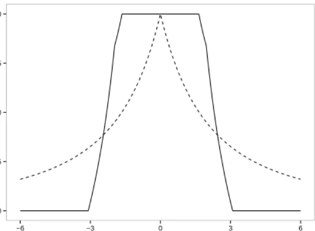
Computation of the M estimators in (10) boils down to iteratively reweighting the least squares estimator. We use the redescending Hampel weighting function giving a good trade-off between robustness and efficiency (Hampel et al., 1986).
ω(x) = 1 |x| ≤a a |x| a <|x| ≤b q−x q−b a |x| if b <|x| ≤q 0 q <|x| , (15)
wherein the tuning constants a, b and q can be chosen as distribution quantiles. For the
residual weight functionωRin (8) we take the 0.95,0.975 and 0.999 quantiles of the standard
0.00 0.25 0.50 0.75 1.00 −6 −3 0 3 6 x w eights
Figure 1: The Hampel (solid) weighting function with standard normal 95%, 97.5% and
99.9% quantiles as cutoffs and the Fair (dashed) weighting function with parameter c= 4.
Note that in the original publication on partial robust M regression (Serneels et al., 2005), the Fair function was recommended (both weighting functions are plotted in Fig-ure 1), but the authors consider the Hampel redescending function superior over the Fair function, because (i) it yields case weights that are much easier to interpret, since they are exactly 1 for the regular cases, exactly 0 for the severe outliers and in the interval (0,1) for the moderate outliers and because (ii) the tuning constants for the cutoffs can be set according to intuitively understandable statistical values such as quantiles from a corresponding distribution function.
The algorithm to compute the SPRM estimators iteratively reweights a sparse PLS estimate. This sparse PLS estimate is computed as in Lee et al. (2011), who outline a sparse adaptation of the NIPALS computation scheme (Wold, 1975), where in each step of
the NIPALS the obtained direction vector of the deflatedX matrix is modified according to
Equation (14) in order to get sparseness. The starting values of the SPRM algorithm have to be robust. Failing to estimate robust starting values, would lead to an overall nonrobust estimator. Algorithm 1 presents the computing scheme and details the starting values.
We iterate until convergence, that is whenever the relative difference in norm between
two consecutive approximations of ˆβ is smaller than a specified threshold, e.g. 10−2. An
implementation of the algorithm is available on CRAN in the package sprm (Serneels and
X and y denote robustly centered data by subtracting the (column-wise) median. 1. Calculate initial case weights:
• Calculate distances for xi (ith row of X) and yi:
di = kxik2 medjkxjk2 and ri = |yi| cmedj|yj| for i∈ {1, ..., n}
where c= 1.4826 for consistency of the MAD.
• Define initial weights ωi =
p ωT(di)ωR(ri) for Ω(see (8)). 2. Iteratively reweighting: • Weight data: Xω =ΩX yω =Ωy
• Apply the sparse NIPALS to Xω and yω and obtain scores Tω, directions Aω,
coefficients ˆβω and predicted response ˆyω.
• Calculate weights for scores and response.
– Center diag(1/ω1, ...,1/ωn)Tω by the median and scale the
columns with the robust scale estimator Qn to obtain ˜T.
– Calculate distances for ˜ti (ith row of ˜T) and the robustly centered and
scaled residuals ri for i∈ {1, ..., n}:
di =
k˜tik2
medjk˜tjk2
ri =
|yω,i−yˆω,i−medk(yω,k−yˆω,k)|
cmedj|yω,j−yˆω,j−medk(yω,k −yˆω,k)|
– Update weights ωi =
p
ωT(di)ωR(ri).
Repeat until convergence of ˆβω.
3. Denote estimates of the final iteration by Aand ˆβ and the scores by T =XA.
4
Model selection
The computation of the SPRM estimator requires specification of hmax, the number of
latent components, and the sparsity parameter η ∈ [0,1) (see Equation (14)). For η = 0
the model is estimated including all variables, for η tending towards 1 almost no variables
are selected.
A grid of values for η is searched and hmax = 1,2, ..., H. With k-fold robust cross
validation the best parameter combination is selected. For each combination of hmax and
η the model is estimated k times based on a training set containing (100−k) percent
of the data, and then evaluated for the remaining data, constituting the validation set. All observations are considered once for validation and so we obtain a single prediction
for each of them. As robust cross validation criterion the one sided α% trimmed mean is
calculated from the squared prediction errors, such that the largest α% errors which may
come from outliers are excluded. We choose the parameter combination where this measure of prediction accuracy is smallest.
The model selection procedure in the following is based on 10-fold cross validation. For the robust methods the one sided 15% trimmed mean squared error is applied as decision criterion and for the classical methods the mean squared error of prediction is used for
validation. The parameter hmax has a value domain from 1 to 5 and for SPLS and SPRM
the sparsity parameter η is chosen among ten equally spaced values from 0 to 0.9.
5
Simulation study
In this section the properties of SPRM and the related methods PRM, PLS and SPLS are studied by means of a simulation study. Training data are generated according to the model
yi =tiγ+ei for 1≤i≤n, (16)
where the score matrix T =XA, for a given matrix of direction vectors A.
LetXbe ann×pdata matrix with columns generated independently from the standard
normal distribution. We generate the columns ah (h = 1, . . . , hmax) of A such that only
into q columns of relevant variables and p−q columns of uninformative variables. The
nonzero part of A is given by the eigenvectors of the matrix XTqXq, where Xq contains
the firstqcolumns ofX. This ensures that the side conditions forahhold (see (11b)). The
components of the regression vector γ ∈Rhmax are drawn from the uniform distribution on
the interval [0.5,1.5]. The errorsei are generated as independent values from the standard
normal distribution. In a second experiment we investigate the influence of outliers. The
first 10% of the errors are generated from N(15,1) instead of N(0,1). To induce bad
leverage points the first 5% of the observationsxi are replaced by vectors of random values
from N(5,0.1). This will demonstrate the stability of the robust methods when compared
to the classical approaches.
In the simulation study mrep = 200 data sets with n = 60 observations are generated
according to (16) for various values of p. While q= 6 is fixed, we will increase pgradually
and therefore decrease the signal to noise ratio. This illustrates the effect of uninformative variables on the four model estimation methods and incorporates low dimensional as well
as high dimensional settings. For every generated data set we compute the estimator ˆβj
(for 1≤ j ≤mrep) with sparsity parameter η and hmax selected as described in Section 4.
Note that the true coefficients βj are different for every simulation run, since every data
set is generated with a different regression vector γ.
Performance Measures: To evaluate the simulation results the mean squared error (MSE) is used as a measure of the accuracy of the model estimation.
MSE( ˆβ) = 1
mrep
X
1≤j≤mrep
kβˆj−βjk2 (17)
Furthermore, let ˆβj0 be the subvector of βj corresponding to the uninformative variables.
In the true model βj0 is a vector of zeros. Nonzero values of ˆβj0 contribute to the model
uncertainty. One main advantage of sparse estimation is to reduce this uncertainty by setting most coefficients of uninformative variables exactly to zero. The mean number of
nonzero values in ˆβj0 is reported for both sparse methods to illustrate whether this goal
was achieved.
The last quality criterion discussed in this section is the prediction performance of
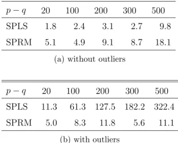
Table 1: Average number of nonzero coefficients of uninformative variables for SPLS and SPRM for simulations with (a) clean training data and (b) training data with 10% outliers.
p−q 20 100 200 300 500
SPLS 1.8 2.4 3.1 2.7 9.8
SPRM 5.1 4.9 9.1 8.7 18.1
(a) without outliers
p−q 20 100 200 300 500
SPLS 11.3 61.3 127.5 182.2 322.4
SPRM 5.0 8.3 11.8 5.6 11.1
(b) with outliers
observations is generated according to the model in each repetition. For 1 ≤j ≤mrep the
estimated response of the test data is denoted by ˆyjtest and the true response is yjtest. Then
the mean squared prediction error (MSPE) is computed as
MSPE = 1
mrep
X
1≤j≤mrep
kˆyjtest−yjtestk2. (18)
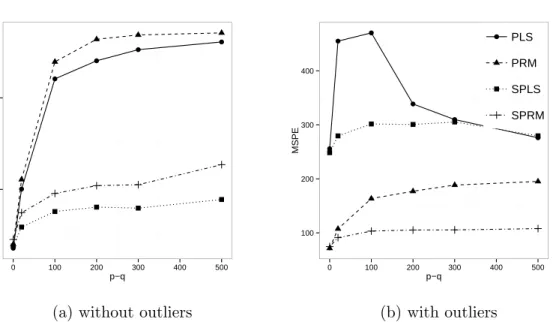
Results for clean data: In the absence of outliers (see Figure 2a and 3a) the overall performance of the classical methods SPLS and PLS is slightly better than for the robust counterparts SPRM and PRM, respectively. In Figure 2a it is seen that the MSE is smallest
for SPLS. If all variables are informative, sop−q= 0, then PLS performs as good as SPLS;
but for an increasing number of uninformative variables PLS quickly becomes less reliable. The same can be observed for the mean squared prediction error in Figure 3a. Both Figures 2a and 3a show that SPRM is not as accurate as SPLS, but performs much better than PLS and PRM for settings with increasing number of noise variables.
Table 1a underpins the advantage of sparse methods. It shows the average number of uninformative variables included in the model, which should be as small as possible. SPLS is better than SPRM, but for both estimates few noise variables are included, leading to reduced estimation error in comparison to PLS and PRM. The MSE for the estimation
● ● ● ● ● ● 0.5 1.0 1.5 2.0 0 100 200 300 400 500 p−q MSE of β
(a) without outliers
● ● ● ● ● ● 0 2 4 6 0 100 200 300 400 500 p−q MSE of β ● PLS PRM SPLS SPRM (b) with outliers
Figure 2: Mean squared error of the coefficient estimates for PLS, PRM, SPLS and SPRM for simulations with (a) clean training data and (b) training data with 10% outliers.
● ● ● ● ● ● 100 150 0 100 200 300 400 500 p−q MSPE
(a) without outliers
● ● ● ● ● ● 100 200 300 400 0 100 200 300 400 500 p−q MSPE ● PLS PRM SPLS SPRM (b) with outliers
Figure 3: Mean squared prediction error for PLS, PRM, SPLS and SPRM for simulations with (a) clean training data and (b) training data with 10% outliers.
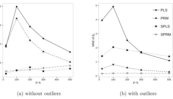
● ● ● ● ● 0.25 0.50 0.75 1.00 0 100 200 300 400 500 p−q MSE of β0
(a) without outliers
● ● ● ● ● 0 1 2 3 4 5 0 100 200 300 400 500 p−q MSE of β0 ● PLS PRM SPLS SPRM (b) with outliers
Figure 4: Mean squared error of the coefficient estimates of the uninformative variables for PLS, PRM, SPLS and SPRM for simulations with (a) clean training data and (b) training data with 10% outliers.
though SPRM has less zero components in ˆβj0. That means that the nonzero coefficient
estimates of the uninformative variables are very small for SPRM. PRM gives surprisingly
good results for the MSE of ˆβ0 and outperforms PLS.
Results for data with outliers: Outliers distort the estimation of PLS and SPLS heavily. Figures 2b and 3b show that the performance of PLS and SPLS strongly deteriorates, while the robust methods are hardly influenced by the presence of the outliers. Further the robust methods behave as expected when the number of uninformative variables increases: The MSE and MSPE for PRM increases remarkably whereas SPRM shows only a slight increase, which marks the advantage of sparse estimation.
In Table 1b it is seen that SPRM includes hardly any uninformative variables in the model whereas SPLS fails to identify the noise variables to a high degree. For all settings
more than half of the noise variables are included. Hence, the estimation of β0 is distorted
for the classical methods as shown in Figure 4b.
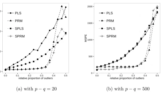
Increasing the number of outliers: An important focus in the analysis of robust methods is to study how an increasing percentage of outliers affects the model estimation. We use
● ● ● ● ● ● ● ● ● ● ● ● ● ● ● ● 0 1000 2000 3000 0.0 0.1 0.2 0.3 0.4 0.5
relative proportion of outliers
MSPE ● PLS PRM SPLS SPRM (a) with p−q = 20 ● ● ● ● ● ● ● ● ● ● ● ● ● ● ● ● 0 500 1000 1500 2000 0.0 0.1 0.2 0.3 0.4 0.5
relative proportion of outliers
MSPE ● PLS PRM SPLS SPRM (b) withp−q = 500
Figure 5: Mean squared prediction error for PLS, PRM, SPLS and SPRM illustrating the effect of increasing number of outliers for data with (a) 20 uninformative variables, (b) 500 uninformative variables.
of outliers. In each step the number of outliers increases by two (one of these two is a bad leverage point) till 50% outliers are generated. The mean squared prediction error as defined in (18) is calculated. Figures 5a and 5b display the MSPE for increasing number of outliers, each graph for a fixed number of uninformative variables.
We observe for the robust methods PRM and SPRM hardly any change in the quality of the prediction performance of the estimated models for up to 33% contamination. The classical methods yield distorted results even for only 3% contamination. Figure 5b show that this high robustness of PRM and SPRM remains when there is a large number of (uninformative) variables. We conclude that the robust methods clearly outperform PLS and SPLS in presence of outliers, while SPRM gives better mean squared prediction error than PRM for percentages of outliers up to 33 percent.
6
Application
Sparse regression methods and big data go hand in hand. Therefore, there are manifold
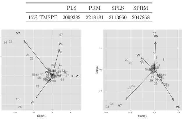
Table 2: Prediction performance for polymer stabilizer data. PLS PRM SPLS SPRM 15% TMSPE 2099382 2218181 2113960 2047858 1 2 3 4 5 6 7 8 9 10 11 12 1314 15 16 17 18 19 20 21 22 23 24 25 26 27 28 29 30 31 32 33 34 35 36 37 38 39 40 41 42 43 44 45 4647 48 49 50 51 52 53 54 55 56 57 58 59 V1 V2 V3 V4 V5 V6 V7 −5 0 5 10 −10 −5 0 5 Comp1 Comp2 (a) PRM 1 2 3 4 5 6 7 8 9 10 11 12 13 14 15 16 17 18 19 20 21 22 23 24 25 26 27 28 29 3031 32 3334 35 36 37 38 39 40 41 42 4351534945484452504647 545655 57 58 59 V4 V5 V6 V7 −2.5 0.0 2.5 −5.0 −2.5 0.0 2.5 Comp1 Comp2 (b) SPRM
Figure 6: The PRM and SPRM biplots for the gloss data example
(Chun and Kele¸s, 2010)), but they have also found their way into chemometrics (e.g. Filzmoser et al., 2012) or medicine (e.g. the application on NMR spectra of neural cells (Allen et al., 2013)). Even though sparse regression methods are of great use when data dimensionality is high, they can already be beneficial when applied to low dimensional problems (which, in the context of classification, has been reported in Filzmoser et al. (2012)). Therefore, in the first example we will focus on data of moderate dimensionality, followed by a gene expression example to illustrate the application to high dimensional data.
The gloss data: The data consist ofn = 58 polymer stabilization formulations, wherein
thep= 7 predictors are the respective concentrations of seven different classes of stabilizers.
The actual nature of the classes of stabilizers, as well as the respective concentrations, are proprietary to BASF Corp. and cannot be disclosed. The response variable targets to quantify the quality of stabilization by measuring how long it takes for the polymer to lose
50% of its gloss when weathered (in what follows, simply called the gloss). The target is to
predict the gloss from the stabilizer formulations. The data were scaled with the Qn scale
for the robust methods (Rousseeuw and Croux, 1993) and for the classical methods with the standard deviation.
PLS, SPLS, PRM and SPRM use the 10-fold cross validation procedure described in Section 4. The optimal number of latent components for PLS and PRM was detected to equal 1. For SPRM the optimal number of latent components is 4 and the sparsity
parameter was found to be η= 0.6; for SPLS we have hmax = 3 andη = 0.9.
To evaluate the four methods leave-one-out cross validation was performed and the one sided 15% trimmed mean squared prediction error (TMSPE) is reported in Table 2. SPRM performs slightly better according to the TMSPE. Another advantage of sparse robust modeling in this example is the interpretability. Figure 6 compares the biplots of PRM and SPRM for the first two latent components. In the sparse biplot variables V1, V2 and V3 are excluded and so it is easier to grasp in which way the latent components depend on the original variables, and how the individual cases differ with respect to the selected variables.
The NCI data: The National Cancer Institute provides data sets of measurements
from 60 human cancer cell lines (http://discover.nci.nih.gov/cellminer/). The 40th
observation has to be excluded due to missing values, i.e. n = 59. The gene expression data
comes from an Affymetrix HG-U133A chip and was normalized with the GCRMA method.
It is used to model log2 transformed protein expression from a Lysate Array. From the
gene expression data only the 25% of the variables with highest variance are considered,
which leads top= 5571, as was similarly conducted by Lee et al. (2011). The protein data
consists of measurements of 162 expression levels. Since the proposed method is designed for univariate response we modeled the relationship for each protein expression separately and obtain 162 models for each of the competitive methods.
As before, the model selection is done using 10-fold cross validation (see Section 4) and the selected models are evaluated with the 15% TMSPE. For each of the 162 different responses the TMSPE of each estimated model is divided by the smallest of the four TMSPEs. This normed TMSPE is a value equal to 1 (for the best method) or larger and
● ● ● ● ● ● ● ● ● ● ● ● ● ● ● ● ● ● ● ● ● ● ● ● ● ● ● ● ● ● ● ● ● ● ● ● ● ● ● ● ● ● ● ● ● ● ● 1.0 2.5 5.0 10.0 PLS PRM SPLS SPRM nor med TMSPE
Figure 7: Boxplots of normed TMSPE of 162 responses from the NCI data for PLS, PRM, SPLS and SPRM.
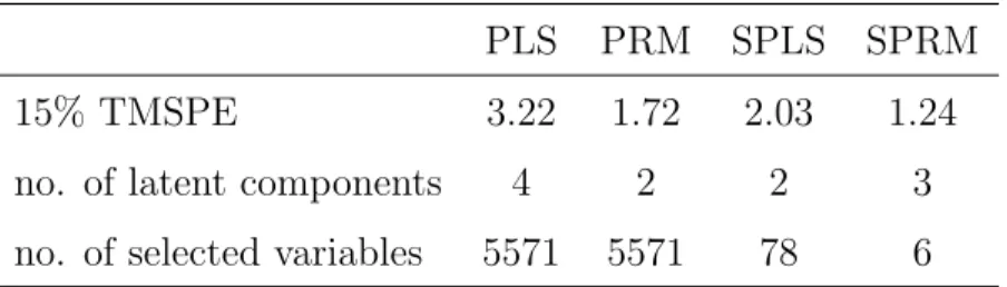
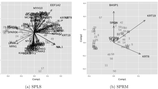
we can compare it across the different responses (see Figure 7). Overall, the combination of sparsity and robustness leads to a superior evaluation. The median of the normed TMSPE of the SPRM models is very close to 1 and therefore we can conclude that for half of the models SPRM is either the best or very close to the best model. PLS is not an appropriate method for these data, since the TMSPE differs strongly from the best model in most cases. For purpose of illustration we focus on Keratin 18 as response. It has the highest variance of all responses and its expression is an often used criterion for the detection of carcinomas (Oshima et al., 1996). Table 3 presents the number of latent components and the number of selected variables (i.e. having nonzero estimated coefficients) for each method, together with the TMSPE. The SPRM model gives the best result with only 6 out of 5571 variables selected. Even PRM performs better than SPLS in this high dimensional setting, which underpins the importance of robust estimation for these data. Figure 8 shows the biplot of scores and directions for the first two latent components of the SPLS and the SPRM model. For SPRM the first latent component is determined by the variables KRT8 and KRT19. The expression of these genes is known to be closely related to the protein expression of Keratin 18 and they are used for the identification and classification of tumor cells (Schelfhout et al., 1989; Oshima et al., 1996). KRT8 has previously been reported to
Table 3: Model properties for NCI gene expression data with protein expression of Keratin 18 as response variable.
PLS PRM SPLS SPRM
15% TMSPE 3.22 1.72 2.03 1.24
no. of latent components 4 2 2 3
no. of selected variables 5571 5571 78 6
play an important role in sparse and robust regression models of these data (Alfons et al., 2013). The biplot further unveils some clustering in the scores and provides insight into the multivariate structure of the data. The biplot of the SPLS model (Figure 8a) cannot be interpreted since this model including 78 variables is too complex. Interestingly, in the SPLS biplot KRT8 and KRT19 are also the genes which have the largest positive influence on the first latent component.
Note that the case weightsωi of the robust models presented in Figure 9 are as expected:
they are one for the bulk of the data, exactly zero for the potential outliers and in the interval (0,1) for a few observations, which is an immediate consequence of adopting the Hampel weighting function (Equation (15) and Figure 1). Hence, outliers can easily be identified. The detection of potential outliers differs between PRM and SPRM, but the pattern is similar.
7
Conclusions
SPRM is a sparse and robust regression method which performs dimension reduction in a manner closely related to partial least squares regression. It performs intrinsic variable selection and retrieves sparse latent components, which can be visualized in biplots and interpreted better than nonsparse latent components especially for high dimensional data. Since sparse methods eliminate the uninformative variables, higher estimation and predic-tion accuracy is attained. The SPRM estimapredic-tion of latent components and the selecpredic-tion of variables is resistant to outliers. To reduce the influence of outliers on the model estimation an iteratively reweighted regression algorithm is used. The resulting case weights can be
1 2 3 4 5 6 7 8 9 10 11 12 13 14 15 16 17 18 19 20 21 22 23 24 25 26 27 28 29 30 31 3233 34 3536 37 38 39 41 42 43 44 4546 47 48 49 50 51 52 53 54 55 56 57 58 59 60 DSP SPARC HSPA1A GPNMB IFITM2 IGFBP4 KRT18 KRT19 FAM127A EPCAM EFEMP1 SRGN SRGN.1 BASP1 SERPINE1 SERPINE1.1 GPX2 HLTF PLA2G2A LAMA3 TSPAN8 QPRT LGALS4 EEF1A2 DKK1 HMGCS2 TFF3 MYB SERPINB5 LCK LCK.1 PFN2 AREG PRSS2IL1R2 CALB1 CALB1.1 MLANA PRSS3 PCK1 FSTL1 KRT8 KRT7 MCAM TFPI2 ANXA3 DUSP5 NA. FN1 SPINT2 MCAM.1 MCAM.2 IL1R2.1 FN1.1 RHOB PBX1 IFITM3 MYH10 RDX NME4 KIAA1199 PRSS3.1 LYZ ARMCX6 PIWIL1TRY6 LPXN NA..1 FN1.2 TRY6.1 NGFRAP1 WBP5 NRN1 PDGFC FERMT1 C3orf14 NA..2 SFN −0.6 −0.4 −0.2 0.0 0.2 0.4 −0.2 −0.1 0.0 0.1 0.2 Comp1 Comp2 (a) SPLS 1 2 3 4 5 6 78 9 10 11 12 13 14 15 1617 18 19 20 21 22 23 24 25 26 27 28 29 30 31 32 33 34 35 36 37 38 3941 42 43 44 45 46 47 48 49 50 51 5253 54 55 56 57 58 59 60 IGFBP4 KRT19 SRGN BASP1 KRT8 PLAC8 −0.2 −0.1 0.0 0.1 0.2 0.3 −0.1 0.0 0.1 Comp1 Comp2 (b) SPRM
Figure 8: The SPLS and SPRM biplots for the gene data example with protein expression of Keratin 18 as response. PRM SPRM 0.00 0.25 0.50 0.75 1.00 0.00 0.25 0.50 0.75 1.00 0 20 40 60 case w
Figure 9: The PRM and SPRM case weights for the gene data example with protein
used for outlier diagnostics.
We demonstrated the importance of robustness and sparsity properties in a simulation study. The method was shown to be robust with respect to outliers in the predictors and in the response and achieved good results for settings with high percentage of outliers. The informative variables were detected accurately. We illustrated the performance of SPRM on a data set of polymer stabilization formulations of moderate dimensionality and on high dimensional gene expression data. An implementation of the SRPM, as well as visualization tools and the cross-validation model selection method outlined in Section 4, is available on
CRAN in the package sprm (Serneels and Hoffmann, 2014).
The extension of SPRM regression for a multivariate response is a next step to take. Note that few papers combine sparseness and robustness for multivariate statistics, an exception is Croux et al. (2013) for principal component analysis. The development of pre-diction intervals around the SPRM prepre-diction is another challenge left for future research. A bootstrap approach seems reasonable, but its validity remains to be investigated. Ob-taining theoretical results on breakdown point or consistency of the model section is out of the scope of this paper. Few theoretical results are available in the PLS literature, and this only for the nonrobust and nonsparse case. In this paper we proposed and put into practice a new sparse and robust partial least squares method, which we believe to be valuable for data scientists confronted with prediction problems involving many predictors and noisy data.
Acknowledgments
This work is supported by BASF Corporation and the Austrain Science Fund (FWF), project P 26871-N20 .
References
Alfons, A., Croux, C., and Gelper, S. (2013). Sparse least trimmed squares regression for
Allen, G., Peterson, C., Vannucci, M., and Maleti´c-Savati´c, M. (2013). Regularized partial
least squares with an application to nmr spectroscopy. Statistical Analysis and Data
Mining, 6:302–314.
Chun, H. and Kele¸s, S. (2010). Sparse partial least squares regression for simultaneous
dimension reduction and variable selection. Journal of the Royal Statistical Society,
72:3–25.
Croux, C., Filzmoser, P., and Fritz, H. (2013). Robust sparse principal component analysis.
Technometrics, 55(2):202–214.
Filzmoser, P., Gschwandtner, M., and Todorov, V. (2012). Review of sparse methods in
regression and classification with application in chemometrics.Journal of Chemometrics,
26:42–51.
Filzmoser, P., Serneels, S., Maronna, R., and Van Espen, P. (2009). Robust multivariate
methods in chemometrics. In Brown, S., Tauler, R., and Walczak, B., editors,
Compre-hensive Chemometrics, volume 3, pages 681–722. Elsevier, Oxford.
Hampel, F., Ronchetti, E., Rousseeuw, P., and Stahel, W. (1986). Robust Statistics: the
approach based on influence functions. Wiley.
Lˆe Cao, K., Rossouw, D., Robert-Grani´e, C., and Besse, P. (2008). A sparse pls for variable
selection when integrating omics data. Statistical Applications in Genetics and Molecular
Biology, 7:35.
Lee, D., Lee, W., Lee, Y., and Pawitan, Y. (2011). Sparse partial least-squares regression
and its applications to high-throughput data analysis. Chemometrics and Intelligent
Laboratory Systems, 109(1):1–8.
Liebmann, B., Filzmoser, P., and Varmuza, K. (2010). Robust and classical pls regression
compared. Journal of Chemometrics, 24:111–120.
Oshima, R. G., Baribault, H., and Caul´ın, C. (1996). Oncogenic regulation and function
of keratins 8 and 18. Cancer and Metastasis Reviews, 15(4):445–471.
Rousseeuw, P. and Croux, C. (1993). Alternatives to the median absolute deviation.Journal
of the American Statistical Association, 88:1273–1283.
Rousseeuw, P. J. and Leroy, A. M. (2003). Robust Regression and Outlier Detection. John
Wiley & Sons, 2nd edition.
Schelfhout, L. J., Van Muijen, G. N., and Fleuren, G. J. (1989). Expression of keratin 19 distinguishes papillary thyroid carcinoma from follicular carcinomas and follicular
thyroid adenoma. American journal of clinical pathology, 92(5):654–658.
Serneels, S., Croux, C., Filzmoser, P., and Van Espen, P. (2005). Partial robust
M-regression. Chemometrics and Intelligent Laboratory Systems, 79:55–64.
Serneels, S. and Hoffmann, I. (2014). sprm: Sparse and Non-sparse Partial Robust M
Regression. R package version 1.0.
Tibshirani, R. (1996). Regression shrinkage and selection via the lasso. Journal of the
Royal Statistical Society, 58:267–288.
Tibshirani, R. (2011). Regression shrinkage and selection via the lasso: a retrospective.
Journal of the Royal Statistical Society: Series B (Statistical Methodology), 73(3):273– 282.
Wold, H. (1965). Multivariate analysis. In Krishnaiah, P., editor, Proceedings of an
Inter-national Symposium 14-19 June, pages 391–420. Academic Press, NY.
Wold, H. (1975). Soft Modeling by Latent Variables; the Nonlinear Iterative Partial Least
Squares Approach. Perspectives in Probability and Statistics. Papers in Honour of M. S.
Bartlett.
Zou, H., Hastie, T., and Tibshirani, R. (2006). Sparse principal component analysis.
FACULTY OF ECONOMICS AND BUSINESS Naamsestraat 69 bus 3500 3000 LEUVEN, BELGIË tel. + 32 16 32 66 12 fax + 32 16 32 67 91 [email protected] www.econ.kuleuven.be