USING ARTIFICIAL INTELLIGENCE TECHNIQUES
Jovan Barac
Submitted for the degree o f PhD at University College London
All rights reserved
INFORMATION TO ALL USERS
The qu ality of this repro d u ctio n is d e p e n d e n t upon the q u ality of the copy subm itted.
In the unlikely e v e n t that the a u th o r did not send a c o m p le te m anuscript and there are missing pages, these will be note d . Also, if m aterial had to be rem oved,
a n o te will in d ica te the deletion.
uest
ProQuest 10609093
Published by ProQuest LLC(2017). C op yrig ht of the Dissertation is held by the Author.
All rights reserved.
This work is protected against unauthorized copying under Title 17, United States C o d e M icroform Edition © ProQuest LLC.
ProQuest LLC.
789 East Eisenhower Parkway P.O. Box 1346
Table of Contents
ABSTRACT ... 2
ACKNOWLEDGMENTS ... 4
TABLE OF CONTENTS ... 5
LIST OF FIGURES ... 9
LIST OF TABLES... 10
CHAPTER I: INTRODUCTION ... 11
1.1 Fault diagnosis: a perspective... 11
1.2 Aim of the research... 13
1.3 Motivation for the research... 14
1.4 Thesis outline... 18
CHAPTER II: A KNOWLEDGE-BASED ARCHI TECTURE FOR FAULT ISOLATION IN COMPLEX DYNAMIC SYSTEMS ... 20
2.1 Introduction... 20
2.2 Major characteristics of fault isolation in complex dynamic system s... 20
2.3 Choosing a KBS architecture for fault isolation in complex dynamic systems ... 23
2.3.1 Rule- based systems (RBS) ... 23
2.3.2 Frame based systems ... 26
2.3.3 The blackboard framework... 29
2.3.4 Summary... 31
2.4 Moving from the blackboard model to a computable framework... 32
2.5 Truth Maintenance Systems (T M Ss)... 33
2.5.1 The concept of T M S ... 33
2.5.2 Benefits of TMSs ... 34
2.5.3 Choosing a TMS ... 35
2.5.4 Assumption-based Truth Maintenance System (ATMS) ... 36
2.6 A blackboard architecture for fault diagnosis ... 42
2.6.1 Overall blackboard structure ... 42
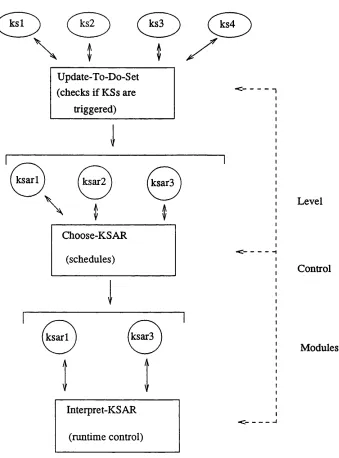
2.6.2 Level control modules ... 44
2.6.3 Overall control m odule... 46
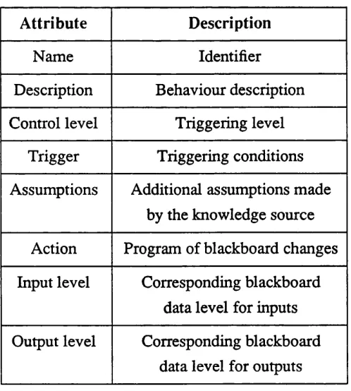
2.6.4 Knowledge sources format... 46
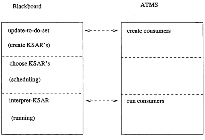
2.7 Interfacing the blackboard and the ATMS ... 47
2.7.1 Interfacing the consumer construct to level control... 47
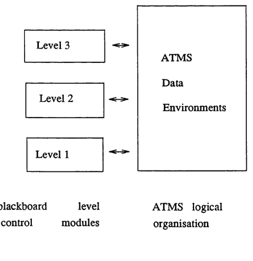
2.7.2 Adapting the ATMS to the proposed control structure ... 49
2.7.3 Using the ATMS to help triggering ... 51
2.8 Comparison to other blackboard architectures ... 54
2.9 Summary... 57
CHAPTER HI: DIAGNOSING SINGLE,MULTIPLE AND SENSOR FAULTS AND REACT ING TO STATE CHANGES ... 58
3.1 Introduction... 58
3.2 Notation and definitions... 58
3.3 Characteristic points of complex dynamic systems... 60
3.4 Existing multiple fault strategies ... 61
3.4.1 Explicit enumeration of possible fau lts... 61
3.4.2 Network Diagnostic System ( NDS ) ... 61
3.4.3 The suspect islands/ clustering approach... 61
3.4.4 Geffher & Pearl ... 63
3.4.5 D a v is... 64
3.4.6 Parsimonious covering theories... 65
3.4.6.1 Single fault restriction... 65
3.4.6.2 Minimal cardinality approach... 65
3.4.6.3 Relevancy ... 65
3.4.6.4 Minimal candidates... 66
3.4.7 Discussion... 69
3.5 Existing sensor fault strategies ... 69
3.6 A new integrated sensor fault/minimal candidate approach... 71
3.6.1 Assumptions ... 71
3.6.2 The meaning of test data... 72
3.6.3 Minimal candidate generation ... 72
3.6.4 Discussion... 78
3.7 Dealing with state changes ... 79
3.7.1 Time information during fault isolation ... 80
3.7.2 State change manifestation... 84
3.7.3 State change /test fault duality... 84
3.7.4 A model for dealing with state changes... 85
3.7.4.1 Suspecting a state change ... 85
3.7.4.2 Testing/confirming a state change ... 88
3.7.4.3 Recovering from a state change ... 89
3.7.4.4 Algorithm refinements... 91
3.7.5 Other approaches to temporal reasoning... 92
3.8 Summary... 94
CHAPTER IV: TEST OPTIMISATION DURING FAULT ISOLATION... 95
4.1 Introduction... 95
4.2 Algorithmic versus heuristic test optimisation... 96
4.3 Assumptions ... 98
4.5 Test optimisation using entropy... 100
4.5.1 Entropy and test generation ... 100
4.5.2 Basic notation and equations ... 100
4.5.3 Candidate probabilities of a failed t e s t ... 103
4.5.4 Entropy of a failed test... 105
4.5.5 Entropy of a successful test ... 106
4.5.6 Total expected entropy of a test... 107
4.6 Terminating a diagnostic session by test biasing... 108
4.7 Heuristics... 109
4.8 Examples... 109
4.9 Discussion... 113
4.10 Review of some existing test optimisation mechanisms ... 114
4.10.1 Arby’s testing methodology ... 114
4.10.2 Sophie’s ad-hoc half split m ethod... 115
4.10.3 Shirley’s testing m ethod... 115
4.10.4 DART ... 116
4.10.5 General Diagnostic Engine (G D E )... 116
4.11 Summary... 116
CHAPTER V: MAPPING THE PROBLEM SOLUTION TO THE ARCHITECTURE... 118
5.1 Introduction... 118
5.2 Fault diagnosis: the ATMS perspective... 118
5.2.1 ATMS reminder... 118
5.2.2 Mapping the problem solution onto the ATM S... 119
5.2.3 Optimising the creation of the assumptions... 124
5.2.4 Optimising the mapping by creating negative assumptions o n ly ... 124
5.2.5 State changes and the ATM S... 125
5.2.6 Summary... 125
5.3 Problem solving; the blackboard perspective... 125
5.3.1 The communication level ... 125
5.3.2 The translation level ... 126
5.3.3 The filtering le v e l... 126
5.3.4 The combination level ... 128
5.3.5 The testing/diagnosis level ... 129
5.3.6 Overall control... 129
5.4 ATMS and blackboard cooperation... 131
5.4.1 The normal data path through the ATMS/blackboard environment ... 131
5.4.2 The state change data path through the ATMS/blackboard environment... 132
5.5 Other issu es... 132
5.5.1 Obtaining continuous diagnosis... 132
5.5.2 Dealing with the knowledge sources... 135
CHAPTER VI: IMPLEMENTATION ISSUES,PRELIMINARY VALIDATION AND FUTURE
WORK ... 136
6.1 Introduction... 136
6.2 Shell implementation status and issu es... 136
6.3 Performance issues ... 137
6.3.1 Fault isolation algorithm characteristics... 137
6.3.2 Average number of iterations ... 139
6.3.3 Minimal candidate generation cost ( t 3 ) ... 145
6.3.4 Calculating the cost of the test evaluation algorithm (t4 )... 148
6.3.5 Average total time taken to perform diagnosis... 150
6.3.6 Issues of parallelism ... 151
6.3.7 Maximum time limit for a diagnosis ... 151
6.3.8 Time taken to deal with state change suspicions... 151
6.3.9 Performance-enhancing heuristics... 152
6.4 Computer networks... 152
6.4.1 Network definition... 153
6.4.2 Network structure ... 153
6.4.3 Network architecture ... 153
6.4.4 Network topologies... 154
6.4.5 Routeing... 157
6.4.6 Network testing to o ls... 157
6.4.7 Important network characteristics ... 158
6.5 Deep knowledge translation of routeing failures into suspect components ... 158
6.5.1 Symptom information and routeing... 159
6.5.2 The statics: Describing the network structure ... 160
6.5.3 The dynamics: Describing the routeing behaviour... 162
6.5.4 Using the network structure and behaviour description to generate suspects... 165
6.5.5 Illustrative ru n s... 166
6.6 Future work on the validation of the proposed shell ... 176
6.7 Conclusion... 178
CHAPTER VH: CONCLUSION... 179
7.1 Thesis summary... 170
7.2 Critical evaluation... 1 n REFERENCES ... 184
APPENDIX 1 ... 189
L ist o f F ig u r e s
1.1 Diagnostic cycle ... 12
2.1 Architecture of rule-based systems ... 23
2.2 I f .. then .. rule exam ple... 24
2.3 A frame node ... 26
2.4 Frame representation ... 27
2.5 Blackboard architecture... 29
2.6 TMS approach to problem solving ... 33
2.7 The proposed blackboard architecture... 44
2.8 Level control procedure... 45
2.9 ATMS/Blackboard correspondence ... 48
2.10 Basic ATMS ... 49
2.11 Split environment ATMS ... 50
2.12 ATMS with separate consumer environments... 51
3.1 Cluster approach to multiple faults... 62
3.2 Mapping to a Bayesian network... 63
3.3 Relevant candidates after measurements... 66
3.4 Minimal candidates after measurements ... 67
3.5 Typical dynamic system ... 81
3.6 Testing c y c le ... 82
3.7 Possible testing sequences... 82
3.8 A simple system ... 83
5.1 State change algorithm and the blackboard levels ... 130
5.2 Blackboard/ATMS interaction ... 133
6.1 Layers, protocols and interfaces... 154
6.2 Computer network topologies... 156
6.3 Black box behaviour... 159
6.4 Hierarchical decomposition of a system ... 160
6.5 Computer network... 162
6.6 Simple network topology... 163
6.7 AND/OR problem decomposition... 165
List of Tables
2.1 Relative merits of rule, frame and blackboard system s... 31
2.2 TMS features ... 34
2.3 Knowledge source format... 46
3.1 Combination example 1 ... 76
3.2 Combination example 2 ... 77
4.1 Entropy example 1 ... 110
4.2 Entropy example 2 ... I l l 4.3 Entropy example 3 ... 112
5.1 Label update/Minimal candidate algorithm duality... 122
6.1 Required number of iterations ... 144
6.2 Total cost of minimal candidate operations... 147
6.3 Total cost of basic test evaluation for the average te s t... 149
INTRODUCTION
I.I. Fault diagnosis: a perspective
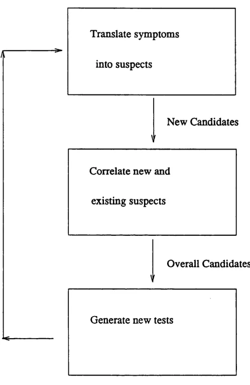
Fault diagnosis is a process whose goal is to determine the fault or faults responsible for a set of symptoms in a particular system [Gene84]. To achieve this goal, diagnostic sys tems repeatedly loop through a three stage cycle [John85]:
Stage 1: Behavioral observations of subsets of the system under observation (SUO) are translated into possible explanations for that behaviour, sometimes called candidates [Davi84] , [Klee87]. Unexpected behaviour is translated into subsets of suspect ele ments, expected behaviour into subsets of "presumed working" elements;
Stage 2: The new explanations for the latest observed behaviour of the SUO, obtained from the symptom translation phase, are combined with the existing explana tions for the previously observed behaviour [Will87], giving a new set of possible expla nations for the observed behaviour of the SUO. Normally the set of possible explanations for the SUO’s behaviour will be a set of alternative fault patterns, each of which can explain all the current symptoms. The combination is normally performed within the confines of a fault model;
Stage 3: The current set of possible explanations is analysed, and new measure ments (tests) which discriminate between the current explanations are suggested and per formed. Usually the best next measurement is the one that will on average lead to the discovery of the faulty set of components in the minimal number of steps [Klee87].
Translate symptoms
into suspects
New Candidates
Correlate new and
existing suspects
Overall Candidates
V
Generate new tests
FIGURE 1.1 Diagnostic cycle
Fault diagnosis can be applied to a wide variety of systems, ranging from simple, static systems such as electronic circuits to complex, dynamic ones such as computer networks. The complex dynamic systems represent the most general category of systems; they are defined as systems consisting of a large number of interconnected components, each of which may change state while being observed. From a diagnostic point of view, a com ponent can be either in a working state or in a faulty state. Normally, the sensors used to observe a complex dynamic system have to be considered as part of the system.
1.2. Aim of the research
The aim of this thesis is to provide a fault diagnostic shell for complex dynamic systems which contains all the elements of fault diagnosis which are system independent. In other words, the shell presented in this thesis supports elements of the fault isolation process which are common and can be generalised to all complex dynamic systems. This system independent shell can then be augmented with domain-specific knowledge every time it is applied to a particular system. The main elements of the dissertation include:
(a) The design of a general, high level architecture suitable for fault isolation in dynamic systems. In the development of the architecture, the main design goals were to make it flexible enough to adapt to all the different stages of fault diagnosis, and to provide as much support as possible to the problem solving requirements, giving the problem solver an opportunity to concentrate solely on the diagnostic reasoning process.
(b) The design of a general fault model for complex dynamic systems. In the develop ment of the fault model, the main design goal was to have a fault model that is sufficiently general and unconstrained to be applicable to any complex dynamic sys tem. Therefore, the model had to be able to deal with single faults, multiple faults, sensor faults and state changes in the system during the fault diagnosis process, all of which can occur in a complex dynamic system.
(c) The design of a general testing strategy for complex dynamic systems. Again the design goal was to build a testing algorithm that is applicable to any dynamic sys tem, and that adapts to changes in the important parameters of the system, rather than relying on the static characteristics of one particular system to decide the optimal tests.
(d) The integration of the proposed fault model and test generation strategy with the high level architecture to provide a fault diagnostic shell for complex dynamic sys tems. The aim here was to show the compatibility of the different design elements and provide a unified tool.
The specific domain chosen for the preliminary validation is that of computer net works and the symptom data relates to connection failures in a computer network. The aim here was to build a research prototype.
1.3. Motivation for the research
Traditionally, computational tools’ progress has followed a two stage cycle of develop ment. In the first stage a system specific solution to a particular problem is worked out. In the second stage, a general solution, sometimes based on system specific solutions, appli cable to a whole class of problems is developed. This pattern already appeared in the ear liest computational tools; Pascal and Leibnitz developed a mechanical calculator to deal with the four basic mathematical operations before Babbage suggested the creation of the first general-purpose computer [Zwas81]. More recently, the pattern was followed in several computer fields. In the development of computer languages, programming in binary code was replaced by by more general and higher level languages such as FOR TRAN, COBOL etc. In operating systems, early system specific operating systems such as Burroughs’ Master Control Program for its B5000 computer [Deit83] were developed before portable, system independent operating systems such as UNIX. In the develop ment of data storage, system specific filing and data access methodologies have been replaced by much more general databases [Mart77]. The reasons for this development cycle are clear; it is easier to work out a problem specific solution and then generalise it to a whole class of problems than to create a general solution for a class of problems that has never been attacked before. Furthermore, general tools normally require much more computer resources, which tend to become cheaper as time goes by.
The one computing discipline where the reverse approach was attempted is artificial intelligence. The first goal of artificial intelligence in the 1960s was to develop general problem solving mechanisms that could solve a whole range of problems, such as the General Problem Solver [Ems69]. In the early 1970s, researchers in artificial intelligence concentrated on general methods for improving problem representation and the search for the solution [Wate85]. Neither of these two periods produced any major break throughs; they were as it were "putting the cart before the horse" by immediately attack ing the most general problem without attempting to first gain experience in a limited subfield.
human behaviour in a very narrow field. These programs were called expert systems and this period corresponds to the expert systems’ vintage period. It produced systems like MYCIN [Shor76], PIP [Pauk76], CASNET [Weis74], INTERNIST-I [Popl75] all assist ing medical diagnosis, PROSPECTOR [Duda79] assisting geological exploration and DENDRAL [Lind80] analysing chemical molecular structures.
The development of the expert system field since then has been much more conventional and has broadly followed the normal trend towards generalisation. First, the problem solving methodologies of the initial systems, implicit within each system, were general ised to problem solving environments, called shells, which can be applied to a whole class of problems. For example, MYCIN was generalised to EMYCIN [VanM79], CASNET lead to EXPERT [Weis79] and PROSPECTOR lead to KAS [Rebo81] Second, new expert system tools were developed, such as OWL [Szol77], KEE [Kunz84], KBS [Redd82], HEARSAY-1H [Balz80] and OPS5 [Forg81] all of which offer particular knowledge representation techniques and specific problem solving techniques. Finally even more general aids have been built, such as ADVISE [Mich83] and AGE [Nii79] which offer a choice of knowledge representation techniques and a choice of problem solving techniques.
As far as fault diagnostic expert systems are concerned, the movement towards generali sation can be analysed from the point of view of the three phases of the fault diagnostic cycle; the translation of symptoms into suspects, the combination of the suspect elements and the requests for new tests.
The translation of symptoms into suspects has been the major research area of diagnostic expert systems. All the early diagnostic expert systems (which were concentrating on medical diagnosis) such as the already mentioned MYCIN, PIP, CASNET and INTERNIST-I used shallow knowledge to perform this translation. Shallow knowledge
is surface knowledge in the sense that rules tend to be heuristic rules of thumb [Cohn85] of the type: "if behaviour A happens, then in 90 % of the cases, such and such com ponents will have failed" [Reit87]. This knowledge is strictly specific to the application in which it is being used and cannot normally be transferred to another system.
the symptoms. Deep knowledge about a system generally means that the system is described through its structure and its behaviour; in such a case the translation of symp toms into suspect components can be performed by running the deep knowledge descrip tion of the system which will yield the system’s expected behaviour and comparing it to the system’s actual behaviour. Compared to shallow knowledge, deep knowledge represents a generalisation because it embodies a methodology for translating symptoms into suspects, applicable to all systems having similar structure and behaviour. Thus all the deep knowledge systems mentioned in the last paragraph incorporate a language for describing the structure and behaviour of digital electronic circuits. However deep knowledge methodologies and languages are currently confined to systems with similar structure and behaviour. For example, a deep knowledge approach suitable for electronic circuits is not suitable for medical problems.
The combination of the suspect elements in the early expert systems in medical diagnosis and electronic troubleshooting such as MYCIN, PEP, DART and CRITTER was made under the simplifying assumptions that there is only one fault in the system, that there are no intermittent faults or state changes and that the sensors cannot go wrong. More recently, expert systems like NDS [Will83] and Williamson’s diagnoser [Will87] have attempted to develop system dependent methodologies for dealing with multiple faults. NDS’s approach depends on the ability to repair a component as soon as it is found to be faulty, and Williamson’s depends on shallow knowledge about the nature of the faults. [Klee87] , [Reit87] and [Peng86] have developed a system independent methodology for dealing with multiple faults in static systems, which takes into account only the results of failed tests. Sensor faults are considered in only a handful of expert systems [Fox83] , [Chan87]. State changes in the system under observation during diagnosis and intermit tent faults are apparently allowed in NDS and Williamson’s diagnoser but the literature does not explain how they are dealt with. We have found no existing system whose fault model includes reasoning about intermittent faults and state changes in the system during diagnosis.
as IDT and DART couple their testing strategies very tightly with a deep knowledge description of the system under observation, thus making the testing algorithm dependent on their particular methodology for translating symptoms into suspects. Furthermore, they do not attempt to optimise the test choice; they just try to generate a reasonable test. Other diagnostic expert systems in computing and engineering such as PDS [Fox83] use shallow knowledge testing methods provided by an expert. SOPHIE, [Brow82] which attempts to split the list of suspects into two sublists of equal probability is geared towards systems with single faults, IN-ATE [Cant83] uses a multi-step lookahead pro cedure (based on the gamma miniaverage methodology [Slag71] ) which is computation ally expensive and GDS [Klee87] adapts the entropy measure to test optimisation in a way which is mainly suited to static systems such as electronic circuits.
Of all the systems mentioned in the review of diagnostic expert systems, GDS stands out as the only system which combines a (deep knowledge) translation of symptoms into suspects with a reasonably general fault model incorporating single and multiple faults and a system independent testing strategy.
The first observation that can be made is that both shallow and deep knowledge diagnos tic systems concentrate mainly on the first part of the diagnostic cycle, namely the trans lation of symptoms into suspects. In fact the name deep knowledge (and shallow knowledge) diagnostic systems is misleading; the deep knowledge normally only applies to one of the phases of the diagnostic cycle. The fault models are almost incidental, and are just used to prove (in the case of deep knowledge models) that the suspect generation phase is correct. The simple fault models would certainly be insufficient for dynamic sys tems; they are also probably insufficient for the domains in question since the single fault assumption is not necessarily tme [Hams83], The non-intermittency assumption and the no-sensor-fault assumption also mean that the whole diagnostic session is monotonic
[Klee87], once data are received there is no need to check, revise or reject them.
This thesis fills the gap in fault diagnostic environments for complex dynamic systems. The approach adopted here differs from most existing approaches. First an attempt is made to redress the balance between the different phases of the diagnostic process by putting much more emphasis on the fault model; the right way to build a diagnostic sys tem should be to decide first on a fault model and then decide on the suspect generation, not the other way round. Second, much more emphasis is put on the test selection algo rithm by trying to optimise it. Third, because the research covers all the phases of the diagnostic cycle, much more emphasis is put on the global architecture of the diagnostic system. Fourth, there is a complete separation between the different phases of the diag nostic cycle. Of all the systems mentioned, only GDS uses a comparable approach. However GDS is geared towards approximately static problems such as electronic cir cuits troubleshooting; the fault model, architecture and testing algorithms developed here apply to the more general category of complex dynamic systems. Finally the proposed diagnostic environment can accept both deep and shallow knowledge based suspect gen eration.
1.4. Thesis outline
The thesis is divided into seven chapters. The present one has explained the aims and motivations of the research.
In Chapter 2, a new high level architecture suitable for fault isolation in dynamic systems is proposed. The architecture is based on the coupling of a blackboard with an Assumption-based Truth Maintenance System (ATMS). The Chapter first describes the motivations for using a blackboard and an ATMS. Then a blackboard configuration suit able for fault diagnosis is developed. This is followed by an explanation of the interface between the blackboard and the ATMS. Finally, some existing architectures are exam ined and the the advantages of the proposed architecture are indicated.
algorithms for recovering from state changes which only reject suspect data. The Chapter is concluded with a summary of existing temporal logics and a discussion of the reasons why they are not appropriate for dealing with state changes in dynamic systems.
In Chapter 4, a new methodology for optimising the selection of the next test to perform, based on the entropy function is proposed. The chapter begins with an examination of existing test selection techniques and points out their shortcomings. Next, the entropy concept is briefly covered. This is followed by the development of the algorithms which show how tests can be evaluated and compared by calculating their expected entropies. Finally examples are given to show that the entropy methodology is not only mathemati cally optimal but also chooses tests which are intuitively appealing.
Chapter 5 shows how the fault model and the testing methodology can be integrated with the blackboard/ATMS architecture to provide a fault diagnostic shell. The Chapter begins by showing how a diagnostic problem is mapped onto the ATMS in an optimal way. Then the diagnostic problem is discussed from the blackboard point of view, in terms of the knowledge sources that form part of the system independent diagnostic shell and in terms of the control mechanisms. Subsequently, the cooperation of the blackboard and the ATMS during the diagnostic process is analysed and the proposed shell extended to deal with continuous diagnosis.
Chapter 6 performs the preliminary validation of the proposed system, and suggests directions for further validation and future work. It begins with a brief discussion of the implementation of the proposed diagnostic shell, followed by its performance evaluation. The next section briefly introduces the field of computer networks, which was the domain chosen as the preliminary testing ground. This is followed by the description of a knowledge source which was used to simulate the translation of symptoms into suspects; the knowledge source translates failed connections between two points of a computer network into a list of network components that may have caused such a failure. Then sample runs from the simulation are given. Then the limits of this preliminary validation are discussed together with the additional steps required for further validation. Finally possible directions for future research and work are given.
Chapter 7 presents the dissertation’s conclusions.
A HIGH-LEVEL ARCHITECTURE FOR FAULT ISOLATION IN COMPLEX DYNAMIC SYSTEMS
2.1. Introduction
The need for Knowledge-Based Systems (KBS) in tasks performed in complex dynamic systems is well documented [Sevi83] , [Wate85] , [Weis83]. The complexity of such tasks, the shortage of human expertise, the lack of general theory, the variability of the data structures make them ideal targets for the KBS approach. This chapter proposes a high-level architecture particularly suitable for building a knowledge-based system for fault isolation in complex dynamic systems. The first part of the chapter analyses the characteristics of fault isolation in complex dynamic systems and concludes that the blackboard model is the most suitable high-level architecture for solving this type of problem. The second part of the chapter proposes a new method for turning the theoreti cal blackboard model into a practical computational entity, based on the coupling of a blackboard with an Assumption-based Truth Maintenance System (ATMS). Subse quently, a new architecture for fault diagnosis in complex dynamic systems is developed. This architecture is based on the blackboard/ATMS coupling and the splitting of the blackboard into layers corresponding to the different stages of fault diagnosis. The inter face between the ATMS and the blackboard and their respective roles within this archi tecture are also analysed.
2.2. Major characteristics of fault isolation in complex dynamic systems
Diversity of knowledge: The task of diagnosing faults is a complex task which needs to integrate a large number of independent sources of knowledge such as knowledge about particular types of faults, knowledge about test generation, knowledge about the combination of the different findings, knowledge about the communication with the sensors etc. These knowledge sources may take many forms such as algorithmic or heuristic, deep knowledge based or shallow knowledge based, procedural or declara tive. This suggests the need for an architecture that facilitates cooperation between many diverse knowledge sources.
The need to cooperate with other tasks: The fault management task is usually not the only task that is performed on a complex system; other tasks may include managing the topology of the system, analysing the performance of the system etc. In systems comprising more than one task, the various tasks need to cooperate; for example the topology manager should provide information about the expected topology of the system to the fault manager, and the fault manager should provide fault data to the performance manager. Therefore, the architecture should facilitate data exchange with other tasks.
Irregularity of data arrival: In a dynamic environment, the data about faults and the state of the system do not arrive in any predetermined way. Faults are reported as they are discovered and the reports may take a variable time to reach the module respon sible for fault management. This suggests an architecture that can easily switch control from one task to another (such as from analysing one report to accepting another report) and preferably one that can perform actions in parallel.
Lack of firm theory of diagnosis: There is no algorithm or theory that specifies "the best way to perform diagnosis" in complex dynamic systems. Some aspects, such as test generation, may be associated with a deep knowledge algorithm and deep knowledge mechanisms have been developed for less complex systems such as digital circuits [Davi84] , [Gene84] , [Klee87]. However the number of possible states and interactions means that diagnosis of complex dynamic systems always has an element of trial and error in it. This again suggests a flexible type of control that can be easily adapted or tuned to attempt a different approach.
Errors in data: Because the sensors are normally themselves part of the complex system under observation, they may go wrong [Fox83]. Therefore the data sent by the sensors may be false. This sensor data property reinforces the desirable system charac teristics mentioned in the previous paragraph.
Changes in the system: A dynamic system changes over time; for example new sensors may be added. The architecture should therefore allow the incorporation of new knowledge sources without any major changes. This suggests an architecture that facili tates the incorporation of new knowledge and has a flexible control mechanism.
Explanation of reasoning: A system that helps a human being or even a fully automated diagnoser needs to be able to explain its conclusions. This suggests a system that facilitates the retracing and the justification of the steps taken during diagnosis.
The need to find all the faults: In many problem spaces, the point of the search is to try and locate one solution to the problem. For example R1 [Breu76] tries to find one good configuration for a proposed computer system. In fault isolation, the point of the search is to find all the solutions, that is all the faulty points. If there are several con current faults, isolating just one of them is an insufficient partial solution. We therefore need an architecture that facilitates the search for all the faults in a system.
The ideal architecture therefore:
1) facilitates cooperation between the different knowledge sources belonging to the task at hand;
2) facilitates data exchange with other tasks;
3) moves easily the focus of attention between different search space points; 4) allows parallel processing of the data;
5) allows easy adaptation to a different diagnostic strategy;
6) can deal with contradictory findings by for example easily retracting its findings; 7) facilitates the incorporation of new knowledge;
8) has no predetermined flow of control; 9) is able to explain its line of reasoning; 10) facilitates the discovery of all the solutions;
2.3. Choosing a high-level architecture for fault isolation in complex dynamic sys tems
fault isolation in complex dynamic systems. Here, the major architectures currently used in knowledge-based systems are described and evaluated according to those criteria.
2.3.1. Rule- based systems (RBS)
Rule-based systems are currently the dominant technique for representing knowledge and making control decisions. They have been used in various fields, including equipment maintenance [Shub82] , fault isolation [Veso83] , process control [Nels82] and geology [Smit83].
Overall architecture
Rule- based systems have three major components: an inference engine (the control), a working memory which contains the case specific facts and a static, long term memory which contains the rules and facts pertinent to the system (the knowledge base). The inference engine builds the current state of the problem solving cycle in the working memory using the knowledge base and dynamic inputs as depicted in Figure 2.1.
The previous section defined the criteria for choosing a problem-solving architecture for
input working rales facts
-3<- memory
data
rales and facts
output
engme
Knowledge representation
RBSs normally incorporate practical human knowledge in conditional if-then rales [Haye85]. A typical rule from the REACTOR system is shown in Figure 2.2.
IF: The heat transfer from the primary coolant system to the secondary coolant system is inadequate
and the feedwater flow is low
THEN: The accident is loss of feedwater
FIGURE 2.2 I f .. then .. rule example
The pool containing the set of these rules and the set of long term facts pertinent to the system is stored in the knowledge base. The case specific facts, relevant to the case that is in progress are stored in the working memory.
Control mechanism
The rules in a RBS are normally used in either or both of the following ways [Weis83] , [Haye85]:
in forward chaining or event driven reasoning the system starts with a subset of evi dence (i.e a small set of facts). These facts satisfy the antecedent ("if') parts of some of the rules which can then be fired (executed), adding the "then" part of the rule to the pool of knowledge. This invocation of the mles proceeds until a satisfac tory conclusion has been reached or until no further mles can be invoked;
in backward chaining the system starts with an initial set of goals. The rules with matching consequents are then examined, and the unmet conditions of the antecedents are defined as the new goals. The system then recursively tries to satisfy these subgoals, until the initial goal has been reduced to a set of subgoals which can be directly satisfied from given information.
Evaluation
While RBSs provide fairly powerful means of data representation and inference, they have several limitations [Bigh87]:
1 They have a fairly rigid form of control; both backward and forward chaining sys tems are at their best when the links are followed sequentially (either when creating an inference chain or backtracking to change some decision previously made). They do not normally provide control mechanisms to jump opportunistically to some other point in the search space. This lack of control flexibility means that:
(a) It is more difficult to volunteer information out of sequence or accept new sen sor readings while the current ones are being processed; both these actions correspond to opportunistic jumps in the search space. RBSs will normally process a piece of data completely before they are ready for the next one. (b) It is difficult to vary the diagnostic strategy. RBSs inference engines are nor
mally centred around an embedded problem space search strategy and varying it can be quite a major task.
(c) It is difficult to adapt the system to parallel processing because the model does not suggest any natural partitioning of the search space. This is because the search space is seen as uniform and monolithic. Of course, it would be possible to search in parallel all the branches of an RBS’s search tree, but this is not
‘intelligent’ parallel processing.
(d) It is difficult to apply one search strategy to a portion of the search space and a different one to a different portion. The model is geared towards one search strategy for the whole problem space and most changes in the inference engine will have global implications.
Points (c) and (d) are influenced by the fact that RBS’s normally view the whole search space as a flat graph and perceive their task as optimised graph search. This corresponds to the founding paradigm of Artificial Intelligence that problem solving is search [Enge88], which is a fairly narrow view of Artificial Intelligence.
3 They do not provide obvious access to the partial solutions by knowledge sources or tasks that are outside the RBS. While it is true that the partial solutions are held in the working memory, RBSs are not normally geared to sharing this information with foreign sources.
As a conclusion, RBS’s do not use sufficiently the "divide and conquer" policy which is beneficial in system design. The only hierarchy in the knowledge about the system is its splitting into rules and facts. This lack of structure in the knowledge space is also reflected in the design of inference engines; they tend to treat the whole search space in a uniform fashion.
2.3.2. Frame based systems
Knowledge representation
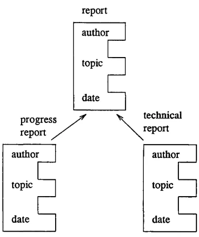
A frame is a network of nodes and relations organised in a hierarchy where the top nodes represent the general concepts and the lower nodes more specific instances of those con cepts. At each node, the concept is defined as a collection of attributes (e.g name, size etc) and values for those attributes (e.g Smith, small etc) Each attribute is known as a slot. Slots can also have procedures attached to them, which may be executed every time a slot is accessed. Typically two types of relationships exist between nodes; member links where an object is linked to a class it belongs to (eg Truckl is a truck) and subclass links where a subdivision of a particular class is linked to that class (eg a truck is a vehi cle) [Fike85], [Wate85]. A typical node and frame are depicted in Figures 2.3 and 2.4.
progress report
if removei if added
procedure Notify author to produce
author report on date
topic
date
Notify author that report is cancelled
procedure
topic
date
technical report progress
report .
author author
topic topic
date date
FIGURE 2.4 Frame representation
Control decisions
Most of the work on frames has focused on their use as a method of representation of data (e.g [Bobr77] , [Brac85] , [Stef79]) rather than on their use for the control of reason ing. In such systems, the frame facility becomes simply a database of the knowledge sys tem; the control decisions are made by other parts of the system. However it is also pos sible to use the frame structure to make control decisions:
Inheritance: The hierarchical structure of frames makes it easy for nodes located lower down in the description hierarchy to automatically inherit the properties of nodes located further up. For example, if all objects in the class "vehicles" have 4 wheels, element "Truckl" which is a vehicle automatically obtains the attribute "has 4 wheels".
Procedural slots: As seen above, it is possible to attach procedures to a slot or a node, which can be executed every time that slot or node is accessed. These procedures can be used to guide the behaviour and thus perform the control of the system. By extension, it is also possible to have full control frames which incorporate procedures only.
the rule in an action slot. This can then be used to group rules into classes and into a hierarchical taxonomy, thus allowing different control strategies for different classes of rules. This is an improvement over pure rule-based systems which do not allow such dif ferentiation.
Overall architecture
Generally in a frame based KBS, control information (i.e the inference engine) and the description of the objects of the system (the knowledge base) are interspersed within the frame hierarchy. The frames model the generic entities and the reasoning process instan tiates the frames for an actual case. In other words, the frame slots are empty at the beginning of the reasoning process whose function is to fill the slots with current values, using procedures, inheritance rule application or any other form of reasoning.
Evaluation
The frame organisation is quite a powerful methodology particularly useful in domains where expectations about the form and content of the data play an important role in prob lem solving, such as classification systems which attempt to classify data according to their type [Wate85]. In such applications, the control path will tend to follow closely the hierarchical frame structure. However, from the point of view of the evaluation criteria developed previously, the frame organisation has several drawbacks:
- there is no clear separation between the control information and the knowledge base; both of them are interspersed in the frame hierarchy. This makes it much more difficult to change the control strategy since it is to a certain extent dependent on the taxonomy of the system under observation;
- the frame model does not suggest any obvious way of performing parallel processing of the data;
- the data is normally stored across the whole frame hierarchy; this makes simultaneous access to data stored in different portions of the frame hierarchy more difficult. It also hinders the exchange of data with outside tasks.
2.3.3. The blackboard framework
Overall architecture
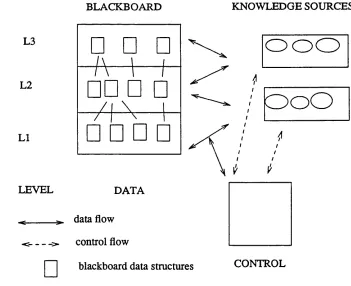
The blackboard architecture normally consists of of three major components [Nii86]:
- A general repository of data called the blackboard which contains all the problem solving state data. This blackboard is often divided into several levels (or layers), each of which contains data relevant to one particular facet of the solution.
- A set of knowledge sources, representing the expertise relevant to the problem, whose role is to manipulate the state data on the blackboard and which cooperate via the black board in the search for the solution.
- A control entity, whose role is to implement a problem-solving strategy.
The overall blackboard architecture is thus as described in Figure 2.5.
BLACKBOARD KNOWLEDGE SOURCES
L3
- / V
□□ □ □
ooo
L2
/ i \ i
□ □ □ □ ^
OoO
LI
V V
LEVEL DA T A
^ data flow
-c >. control flow
blackboard data structures CONTROL
Knowledge representation
The knowledge representation in a blackboard has two aspects; the representation of static, long term knowledge about the problem and the representation of dynamic knowledge corresponding to the current knowledge about the actual case in progress. The dynamic repository of data is the blackboard, containing the partial solutions achieved so far (i.e recording the state of the search so far). In the blackboard model, the long-term domain knowledge is encoded within a set of independent knowledge sources. Each of these knowledge sources is a specialist for some specific aspect of the problem. Within each knowledge source, the knowledge representation can take any form, such as algo rithmic, heuristic etc. Each knowledge source has access to the blackboard. It is triggered by (i.e can contribute to) a particular type of data on the blackboard and if requested transforms it to give new data. The knowledge sources always take their data from the blackboard and always return the enhanced data to the blackboard. If the blackboard is divided into levels, each knowledge source is linked to one or more specific levels.
Control decisions
The role of the control is to coordinate the activities of the knowledge sources and guide the search for a solution. The control entity does this by determining the focus of atten tion that indicates the next thing to be processed. The focus of attention can be the knowledge sources (which knowledge source to activate next) or the blackboard (which data objects on the blackboard to pursue next). The control module can use any of a number of problem-solving strategies: backward chaining, forward chaining, request driving (that is trying to provide information requested by the knowledge sources) etc.
Evaluation
The blackboard model potentially offers all of the following:
the possibility of easy change of focus and easy change of diagnosing strategy; this is because the model does not specify either a specific focus of attention or a preset control path;
easy cooperation between the knowledge sources, with outside tasks, and easy incorporation of new knowledge sources via the blackboard structure where the data can easily be made available;
easy retracting of findings since all the data is on the blackboard;
the possibility of explaining the reasoning since all the data obtained during the rea soning process is available on the blackboard;
the possibility of finding all the solutions to the problem; this is because the black board model is general enough not to put any constraints on the method of searching the problem space.
The blackboard model can therefore satisfy all the criteria for a fault isolation system.
2.3.4. Summary
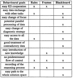
Of the three major high-level architectures, only the blackboard model satisfies all the evaluation criteria and is thus the one we have chosen for our system. The achievement of the behavioral goals by the alternative architectures is summarised in Table 2.1.
Behavioural goals Rules Frames Blackboard
easy KS cooperation X X X
easy data exchange
with other tasks X X
easy change of focus X
potential parallel
processing of data X
easy change of
diagnostic strategy X
easy access to all
the data X X
good treatment of
contradictory data X
easy introduction of
new knowledge X X
no predetermined
flow of control X X X
recording of the
reasoning process X X X
easy path to the
whole solution space X
2.4. Moving from the blackboard model to a computable framework
The blackboard architecture as presented so far only outlines the organizational princi ples and is therefore only a model in the sense given by [Nii86]. It does not specify how to translate the model into a computational entity. Several design decisions have to be taken in order to obtain a computable framework.
The knowledge sources
Decisions to be made about the knowledge sources include:
a) the representation of the knowledge sources; in principle any representation (pro cedural, rules, logic-based etc) can be used;
b) the trigger of each knowledge source; that is the state in which the blackboard has to be for the particular knowledge source to be able to contribute to the general pool of knowledge. Knowledge sources look for specific data on the blackboard;
c) the action of each knowledge source; the action normally results in new data being added to the general pool of knowledge;
d) the interface between the knowledge sources and the blackboard; this interface allows the knowledge sources to write on and read from the blackboard.
The blackboard data
Decisions to be made regarding the blackboard data include:
e) the division (if any) of the blackboard into levels corresponding to the stages of the problem solving process;
f) the objects i.e data to be stored on the blackboard;
g) the relationships between the objects stored on the blackboard, i.e the record of the inference chains followed so far.
The blackboard control
Decisions to be made regarding the blackboard control include:
the organisation of control modules, i.e how they interact, and how the flow of con trol is formed and maintained;
j) the selection of a focus of attention (i.e the next thing to be processed [Nii86]). The focus of attention can be the knowledge sources, the partial solution data on the blackboard or both. This will determine when and how the knowledge sources are triggered and scheduled and also implicitly how the focus of attention will switch between various points of the search space.
The following section shows how several of those requirements are provided by Truth Maintenance Systems (TMSs), which solve them in a uniform, structured and consistent way. Additionally, TMSs also provide some of the other desirable characteristics intro duced in section 2.2.
2.5. Truth Maintenance Systems (TMSs)
2.5.1. The concept of TMS
The methodology of TMSs was first introduced by Doyle [Doyl79] , as a way of improv ing the efficiency of the search of problem spaces, and especially providing a structured way of searching a problem space. The idea is to divide the problem solver into two separate entities; one only concerned with the rules of the domain (The Problem Solver proper) and the other only concerned with recording the current state of the search (i.e the TMS), as depicted in Figure 2.6.
Justifications
Problem
---Solver
Beliefs
<
---TMS
FIGURE 2.6 TMS approach to problem solving
space is ultimately characterised by the set of assumptions under which it is valid (the context).
2.5.2. Benefits of TMSs
By definition [Klee86], all TMSs provide the following services:
an interface to the data and inferences contained in the TMS.
a permanent cache of all the inferences and assumptions ever made, with the infer ence chains that were followed;
a method of switching the focus of attention between the search space points;
a record of the consistency of the data, i.e the TMSs record all the contradictions that have been discovered during the problem solving;
a method of dealing with inconsistent data (be it by eliminating inconsistencies or tolerating them);
The interface to the data and inferences already made can be used to offer direct support to the interface between knowledge sources and the blackboard (requirement d in Section 2.4). The record of all the inferences, inference chains and assumptions directly supports the need to record the relationships between the blackboard objects (requirement g in Section 2.4). The method for switching the focus of attention directly supports the black board control requirement for selecting and switching the focus of attention (requirement j in Section 2.4). The last two services contribute to a good treatment of contradictory data which was one of the ideal architecture characteristics listed in Section 2.2.
Therefore coupling a TMS to the blackboard already provides some of the requested architecture features. The TMS services are summarised in Table 2.2.
- a way of recording the inferences made;
- a way of explaining how the inferences where achieved; - a way of retrieving the data;
- a method of switching between different points of the search space; - a way of dealing with inconsistent data.______________________
2.5.3. Choosing a TMS
Several truth maintenance systems have been developed (TMS [Doyl79] , RUP [McA180] , [McDe83] , MBR [Mart83] , ATMS [Klee86a] , [Klee86b] , [Klee86]). A detailed appraisal of the different TMSs can be found in [Klee86]. For the purpose of fault diagnosis, the ATMS seems to have the best features, because it provides:
an explicit representation of the context in which the data is valid: this is done by associating with each piece of data the assumptions under which the data is valid. In other TMSs this context is only implicit. This facilitates the checking of the validity and the consistency of the data and further contributes to the good treatment of con tradictory data;
a way to switch contexts without backtracking: because the contexts under which the data are valid are kept explicitly with the data, switching contexts simply means starting work on another piece of data. In other TMSs, the system has to backtrack via the inference links to return to a previously reached point in the search space and find the context under which it was valid. This avoidance of backtracking facili tates the change of the focus of attention;
a way to follow mutually contradictory search paths in parallel; because the con texts are explicit there is no reason to insist that all the data in the database are con sistent. Other TMSs insist that all the data be consistent, hence all the backtracking to reach a consistent state. The benefits of non consistent data are clear for our pur poses; for example if a test q finds that element A is faulty, then either q is faulty or A is faulty; the ATMS allows both these (mutually exclusive) facts to be present in the database, and to continue the search in both directions. Other TMSs would require the elimination of one of the two from the set of currently believed data. This facilitates the easy access to all the data;
a way of finding all the solutions at the same time. This is again achieved by allow ing searching in multiple contexts; other TMSs can only find one solution at a time. the possibility of parallel processing; the ATMS is an inherently parallel searching tool, and potentially allows parallel searching of the different contexts.
2.5.4. Assumption-based Truth Maintenance System (ATMS)
The ATMS is described in detail in [Klee86a] , [Klee86b] , [Klee86]. Here only an over view is given.
Architecture
As all TMSs, the ATMS forms part of a two component reasoning architecture: a prob lem solver and an ATMS, as depicted in Figure 2.6. The role of the ATMS is to deter mine belief and disbelief given the justifications supplied so far, and not with respect to the logic of the problem solver. For example, if the problem solver deduced fact A, then made the inference that A implies B and later determined that B is false (all of which were communicated to and recorded by the ATMS), the ATMS would deduce that A is false from the justification that A implies B without understanding the meaning of A and B or the reason why A implied B.
Definitions
The ATMS stores problem solver data in nodes. An ATMS node has several fields, described later, one of which is reserved for the problem solving datum. A new ATMS node is created every time a new problem solver datum is communicated to the ATMS.
An ATMS assumption is a particular type of node, designating the decision to assume. A new ATMS assumption is created every time the problem solver decides to make an assumption in the world in which it is reasoning.
An assumed datum is a problem solver datum that is assumed to hold. It is linked to an
ATMS assumption via a justification as will be shown later.
An ATMS justification describes how the node is derivable from other nodes. The justification of a node N is made of three parts. The first part holds the antecedents of N, that is the nodes used to justify N. The second part holds the consequents of N, that is the nodes in which N was used as an antecedent. The third part holds the Problem Solver’s description of the justification, called the informant which is used for interfacing with the ATMS as will be explained in the interfacing section.
An ATMS environment is a set of assumptions. An environment is consistent if its assumptions are mutually compatible, i.e if there is no contradiction when all its assump tions hold.
An ATMS context is formed by the assumptions of a consistent environment and all the nodes derivable from those assumptions.
The ATMS is thus provided with assumptions and justifications and its role is to efficiently determine the contexts. To this end, the ATMS associates with every datum a succinct description of all the contexts in which the datum is valid, called the label.
Labels
The ATMS associates a label with every node. A label is a set of environments. Every environment E of node N ’s label is consistent and N must be propositionally derivable from E’s assumptions and the current set of justifications given to the ATMS. In contrast to the justification which contains immediately preceding antecedents, the label describes how the datum ultimately depends on assumptions. The label is computed by the ATMS every time a new inference is made. The ATMS guarantees that the label is:
consistent; a label is consistent if all its environments are consistent, i.e if no environment of the label is a superset of an inconsistent environment;
sound; a label is sound if the datum is derivable from each environment of the label; complete; a label is complete if every consistent environment E in which the node holds is a superset of some environment of the label;
minimal; the label is minimal if no environment of the label is a superset of any other.
environment of the label. The basic operations on the label will be discussed a bit later.
Basic data structures
The basic data structure of the ATMS is the node, containing a node identifier, the prob lem solver datum, the label and the justifications:
NodeId:< Datum, Label, Justifications >
There are four types of nodes (distinguished only by their label and justification patterns).
Premises, which hold universally (having the empty environment as justification).
Assumptions, which are self justified; they correspond to the decision to assume, without
any commitment as to what is assumed, as described above.
Assumed nodes, which are justified by an assumption; the assumed node contains a Prob
lem Solver assumed datum.
Other nodes, which are derived.
One distinguished node holds all the inconsistent environments, which are called
nogoods. All the supersets of ’nogood’ environments are also inconsistent. The set of
’nogood’ environments is known as the ’nogood’ database.
For example, let us assume that the problem solver has thus far made three assumptions; x+y=l ;
x=0; x=l.
1:<A,{{A}},{{1} },{4}> 2:<B,{{B}},{{2}},{5}> 3:<C,{{C}},{{3}},{6}> 4:<x+y=l,{ {A}},{{1} },{7,8}> 5:<x=l,{ {B}},{{2}},{7}> 6:<x=0,{ {C}},{{3}},{8}> 7:<y=0,{ {A,B}},{{4,5}},{}> 8:<y=l,{ {A,C}},{{4,6}},{}>
Nodes 1,2 and 3 are ATMS assumptions. Nodes 4,5 and 6 are assumed nodes. Nodes 7 and 8 are deduced nodes. The environment {B,C} is a ’nogood’, since it corresponds to the assumptions x=l and x=0, which cannot be simultaneously true. The environment {A,B} corresponds to making the assumptions that x+y=l and x=l. The environment {A,C} corresponds to making the assumptions that x+y=l and x=0. Nodes 1,4 and 7 are all in the same context {A }. Similarly nodes 2,5 and 7 are all in the same context {B }.
The set of nodes can logically be separated into four non-overlapping sets:
- The true set containing premises;
- The in set containing nodes that hold in at least one currently consistent environment. A consistent environment may later be discovered to be inconsistent;
- The out set containing nodes whose label is empty; they do not currently hold in any known consistent environment but may do so at a later stage;
- The false set containing nodes whose datum is known to be false.
Basic operations and algorithms
The basic operations are the creation of an ATMS node (which is trivial), the creation of an assumption (which is trivial) and the addition of a justification to a node which can cause significant processing, because the ATMS has to construct the new label. The new label is constructed as follows:
2 - This sound and complete label is then made consistent and minimal by eliminating inconsistent and subsumed environments.
The new label (if different from the old one) is then recursively propagated to the conse quent nodes. If however the problem solver indicated that the new node is inconsistent, all the environments of the label are added to the ’nogood’ database, and all the supersets of those environments are eliminated.
For example, let the ATMS currently contain the following data:
l:<x+y=l,{ {A,B},{B,C,D} },{..}> 2:<x=l,{ {A,C},{D,E} },{..}> nogood {A,B,E}
From x+y=l and x=l, the Problem Solver concludes that y=0 and tells the ATMS to create a new node, whose datum is y=0 and whose justification are nodes 1 and 2. To cal culate the label of node 3, the ATMS:
1) Creates a sound and complete label using the algorithm above, giving: {{A,B,C},{A,B,C,D},{ A,B,D,E},{B,C,D,E}}.
2) This sound and complete label is then made consistent by eliminating {A,B,D,E} which contains the inconsistent {A,B,E} and {A,B,C,D} which is subsumed by
{A,B,C}.
3) Node 3 therefore becomes:
3:<y=0,{ {A,B,C},{B,C,D,E} },{(1,2)}>
The notion of classes
Interfacing
The ATMS is accessed via consumers. A consumer is a rule which does some problem solving on the data. A consumer is attached to one or more nodes and run when appropri ate. It is never rerun since the data it is run on can never change. The two basic opera tions on a consumer are creating a consumer and running a consumer.
A consumer is created at the request of the Problem Solver, when the Problem Solver finds that it can make an inference. It informs the ATMS of the set S of nodes that form the basis of the inference and gives a description D of how this inference is to be per formed. The ATMS then creates a new consumer node N whose antecedents are the nodes in set S and whose informant is D, calculates N’s label in the usual way and attaches a consumer to node N. A consumer node is different from the ordinary nodes in two ways; first it has a consumer attached to it and second its datum field is empty.
A consumer is run by consulting the informant and performing the prescribed operation on the list of antecedent nodes.
The reason for having an informant field in the node now becomes clear. It facilitates the separation between the creation of a consumer and the execution of a consumer, i.e the separation between the realisation that an action can be performed and the decision to perform the action. This forms the core of the scheduling operation whose role is to determine which of the possible actions to undertake.
Access paths to the data offered by the ATMS The ATMS offers:
A list of all the nodes together with the associated environments in which they hold; A list of all the classes with associated nodes;
A list of all the consumers with the environments in which they can be run.
Conclusion
The basic ATMS therefore offers to a Problem Solver a method of recording the inferred data, a method of accessing the inferred data, a full record of the way the inferencing was performed, hooks for the triggering, scheduling and running of the different phases of the problem-solving process and a complete methodology for working with multiple contexts and dealing with inconsistent data. As such, it is a powerful tool that solves many design problems of the blackboard.
2.6. A blackboard architecture for fault diagnosis
2.6.1. Overall blackboard structure
The problem of fault diagnosis in complex systems naturally divides itself into several qualitatively different phases:
1 a communication stage where the fault reports are received;
2 a translation stage where the fault reports are translated into the implicated objects; 3 a filtering stage where all the expected findings are justified;
4 a combination stage where new findings are combined with existing findings;
5 a testing diagnostic stage where new tests to discriminate between the suspects are suggested or where the final diagnosis is made.