Defensive
Signal
Processing:
T
he
Case
for
the
Use
of
Nonparametric and Robust Statistical Methods to Reduce
Product Liability Exposure
Michael Lang1,∗
1 Graduate School of Excellence Computational Engineering, Technische Universtät Darmstadt, Dolivostraße 15,
64293 Darmstadt, Germany; Tel.:+49 6151 1624401, Fax: 49 6151 1624404 ∗Correspondence: [email protected]
Abstract: This paper makes the case that in an Internet of Things (IoT) world where data processing has become pervasive, the assessment of whether or not the underlying (statistical) modeling assumptions are justified and appropriate should no longer be limited to the perspective of mathematical statistics alone. The paper argues that large parts of sound academic research in engineering lack practical merit in that, akin to a concept car, they are not market-ready, most commonly due to feasibility and liability issues. Through an analysis of both statistical and legal aspects it will be shown that the stoic pursuit of ‘optimality’ more often than not yields to risky and suboptimal outcomes when applied to actual physical world problems. To address this, the concept of ‘Defensive Signal Processing’ is introduced and future research directions are briefly outlined.
Keywords: defensive signal processing; robust statistics; nonparametric statistics; model uncertainty; IoT; optimization; liability; tortious product liability; strict product liability
1. Introduction
IoT, Big Data, Machine and Deep Learning and related technologies first and foremost leverage the power ofStatistics, a discipline which may be described as the art and science of the analysis and interpretation of data. A crucial commonality encountered in all statistical endeavors lies in the necessity to impose modeling assumptions, be they explicit or implicit in nature, on the observed data.
As will be shown in Section2and exemplified by the pitfalls of the ubiquitous Gaussian assumption, the detrimental ramifications arising from an adherence to unrealistic modeling assumptions have been known for centuries and eventually led to the development of the field of robust statistics and formal robustness theories in the early 1960s. Somewhat ironically however, the stoic quest for optimal robust procedures made them vulnerable to some of the same perils they initially set out to tackle. Nonparametric and distribution-free approaches on the other hand, while being more broadly applicable, are frequently dismissed as too conservative and poor performing.
The main focus of this paper however is not to reiterate decades-old debates pertaining to philosophical aspects of mathematical statistics, which is why Section2is exemplary and purposely non-exhaustive.
While acknowledging the various pros and cons, the first contribution of this paper is to argue that the issue runs deeper and has implications far beyond having to choose between different statistical schools of thought. To substantiate this assertion, Section3will analyze the essentially threefold structure of civil liability for product defects (wherein the focus will be on the German jurisdiction, although due to European harmonization most aspects hold for all European Member States and can furthermore partly be extrapolated to other parts of the world) and emphasize that, unbeknownst to many in the engineering community, civil liability for defective products cannot simply be excluded through general terms and conditions or other means and ought therefore be taken into account from the very early stages of product design and development.
In fact, liability waivers are, at least under European law, generally invalid and may even result in further liability as they may be construed to constitute unfair competition practices. The same is of course true for misleading and/or false advertising claims, whether of direct or implied nature. Furthermore liability waivers
would require a contractual or at least quasi-contractual relationship, neither of which is required for statutory liabilities.
Finally, having established the necessary statistical and legal concepts in Sections2 and3, this paper’s second contribution addresses the research gap in signal processing and related disciplines, where to the best of the author’s knowledge issues of product liability exposure have not systematically and diligently been treated yet, let alone have possible mitigation and defense strategies been proposed. Section4aims to close parts of this gap by devising strategies and techniques for signal processing algorithm design and development characterized by due appreciation of all relevant (interdisciplinary) constraints to eventually reduce the existential risks arising from product liability exposure.
Section5concludes this paper with a discussion and an outlook on future work.
2. Statistical Approaches
In the following basic concepts will be introduced together with the historical context in which they arose. While undoubtedly of great general interest and importance on their own, the at times rather lengthy treatment of selected areas of the history of statistics serves to corroborate the premise that despite their popularity and widespread reliance upon, the unfoundedness of assumptions such as normality have been known for centuries.
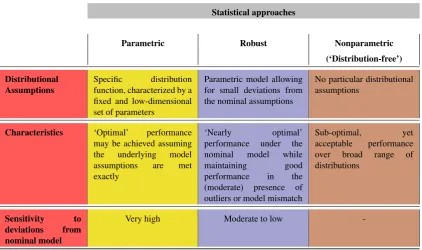
Customarily a distinction between parametric and nonparametric approaches is drawn, representing approaches that favor efficiency over validity and vice-versa, respectively, as depicted in Table1.
Table 1.Overview of statistical approaches: Parametric, Robust, Nonparametric
Statistical approaches
Parametric Robust Nonparametric
(‘Distribution-free’)
Distributional Assumptions
Specific distribution function, characterized by a fixed and low-dimensional set of parameters
Parametric model allowing for small deviations from the nominal assumptions
No particular distributional assumptions
Characteristics ‘Optimal’ performance may be achieved assuming the underlying model assumptions are met exactly
‘Nearly optimal’ performance under the nominal model while maintaining good performance in the (moderate) presence of outliers or model mismatch
Sub-optimal, yet acceptable performance over broad range of distributions
Sensitivity to deviations from nominal model
Very high Moderate to low
2.1. Normality Assumption, Maximum Likelihood and Least Squares
Consider the basic problem of observing a fixed but unknown valueµcontaminated by random errorsXn, i.e.
Yn=µ+Xn (1)
withXn∼ N
0,σ2and thusYn ∼ N
µ,σ2, i.e. the probability density function (p.d.f.) of the random variableYis given by
fY(y) = 1 √
2πσexp
−(y−µ)
2
2σ2
(2)
which may also be written asfY(y;θ)withθ= h
µ,σ2ibeing the finite set of distributional parameters or distributional parameter vector that completely specifies the p.d.f.
The construction of an estimator shall be exemplified by illustrating the maximum-likelihood and least-squares approach to obtainµˆ.
2.1.1. Maximum Likelihood Estimator
The standard method for obtainingµˆin the above-mentioned estimation problem is given by the maximum likelihood approach and was introduced by R. A. Fisher in 1922 [1]. For a detailed (and exciting) historical account reference to Stigler’s paper [2] on ‘the epic history of Maximum Likelihood’ is hereby made.
Given n = 1,. . .,N i.i.d. observations y1,. . .,yN of Yn, the joint probability density function is given by the product of the individual densities, i.e.
f(y1,. . .,yN;θ) = N Y
i=1
f(yi;θ) =L(θ;y) (3)
withL(θ;y)being the likelihood function, a function of the unknown distributional parameter vectorθ conditioned on the observed data sampley= [y1,. . .,yN].
The likelihood functionL(θ;y)can be interpreted as pertaining to the probability of observing exactly the specific dataset at hand, i.e. y1,. . .,yN, for a particularθ. Then, searching for estimatesθˆsuch thatL
ˆ θ;yis maximized yields parameters for the assumed distribution that result in the highest probability of ‘producing’ the observed data.
Since the natural logarithm is a monotonically increasing function, maximizing the more tractable lnL(θ;y)yields to the same result as maximizingL(θ;y). Accordingly, rather than working with the likelihood function of Eq. (3) one conventionally works with the log-likelihood function
lnL(θ;y) = N X
i=1
lnf(yi;θ) (4)
instead. Applied to the problem formulated in Eq. (1) this yields
lnL(θ;y) =−N
2 ln(2π)−
N
2 lnσ
2−1
2 N X
i=1
(yi−µ)2 σ2 (5)
The so-called likelihood-equation provides the necessary condition for maximizing the log-likelihood function, namely
∂lnL(θ;y)
∂µ =
1
σ2
N X
i=1
(yi−µ) =0 (6)
∂2lnL(θ;y)
∂µ2 =−
N
σ2 <0=⇒maximum (7)
holds, the maximum likelihood estimate forµis then obtained by multiplying Eq. (6) withσ2and solving forµˆ, which yields
ˆ µML =
1
N N X
i=1
yi=y (8)
2.1.2. Least Squares Estimator
Alternatively, one may follow a least-squares approach and construct an estimator that minimizes the`2
norm, i.e.
ˆ
µLS=arg min
µ d(µ) =arg minµ N X
i=1
(yi−µ)2 (9)
To determine the estimate that minimizes the distance function
d(µ) = N X
i=1
(yi−µ)2= N X
i=1
y2i −2µ N X
i=1
yi+Nµ2 (10)
one again takes the first derivative and sets it to zero
d0(µ) =−2 N X
i=1
yi+2Nµ=0 (11)
and since
d00(µ) =2N>0=⇒minimum (12)
holds this yields
ˆ µLS =
1
N N X
i=1
yi =y (13)
Thus, if the normality assumption holds, both maximum likelihood and least squares yield the same estimator, in this case the sample mean. Note that this is not generally the case.
2.2. History of the Normal Distribution and long-held Doubts as to the Validity of the Normality Assumption
The optimality of the sample mean (i.e. the arithmetic mean) as an estimate ofµin Eq. (1) should come as no surprise, for the normal distribution was explicitly invoked by Gauss to justify the use of the arithmetic mean.
2.2.1. Historical Background of the Normal Distribution
In his seminal 1809 work titled “Theoria motus corporum coelestium in sectionibus conicis solem ambientium” (Latin for “Theory of the motion of the heavenly bodies moving about the sun in conic sections”), a contribution to the application of mathematics to astronomy, Gauss provides that
It shall not go unmentioned that in his ‘Theoria motus’ Gauss also claimed the discovery of the method of least squares, thereby enraging Legendre who had published said method four years earlier and claimed priority, eventually inciting - to put it in the words of Stigler ([4], p. 465) - “the most famous priority dispute in the history of statistics”. It appears that Gauss had indeed discovered the method well before Legendre but failed to share the discovery with the broad community at the time [4–7].
Huber quotes Gauss from a 1821 paper as stating that
The author of the present treatise, who in the year 1797 first investigated this problem according to the principles of the theory of probability, soon realized that it was impossible to determine the most probable value of the unknown quantity, unless the function representing the probability of the errors is known. But since it is not, there is no other recourse than to assume such a function in a hypothetical fashion. It seemed most natural to him to take the opposite approach and to look for that function which must be taken as a base in order that for the simplest of all cases a rule is obtained which is generally accepted as a good one, namely that the arithmetic mean of several observations of equal accuracy for one and the same quantity should be considered the most accurate value. This implied that the probability of an error x must be assumed proportional to an exponential expression of the form e−hhxx , and that then just the same method which he found by other considerations already a few years earlier, would become necessary in general. This method, which afterwards, in particular since 1801, he had almost daily opportunity to use in diverse astronomical computations, and which in the meantime also Legendre had happened upon, now is in general use under the name method of least squares.([8], p. 1042)
Unbeknownst to some, the normal distribution was actually first introduced by Abraham de Moivre in 1733 as a means of approximating the binomial distribution [7,9]. “He [de Moivre] was actually the first to discover the normal curve (Pearson, 1924), although the credit is usually given to Carl Freidrich [sic] Gauss (1777-1855). In all fairness, it must be mentioned that de Moivre recognized neither the universality nor importance of the normal curve he had discovered” ([7], pp. 95-96). Furthermore, Irish-American mathematician Robert Adrain is believed to have discovered the normal distribution independently of Gauss in 1808, concurrently with his derivation of the method of least squares (the latter however bears striking resemblance to Legendre’s derivation) [10].
In his derivation of the normal distribution Gauss built on previous attempts by Laplace to formally justify the use of the sample mean as the optimal estimator for observations contaminated by random errors, an approach customarily used at the time across the entire spectrum of natural sciences despite the lack of formal justification [6].
While by minimizing the absolute value of the estimate’s deviation from the true value Laplace failed to prove the optimality of the arithmetic mean he ended up proving the median to be the minimum-variance estimator of the location parameter for the double exponential distribution1, whose p.d.f. is given by
fY(y) = m
2 exp[−m|y−θ|] (14)
with 0<m<∞.
Laplace (1774) had formulated the principle for parametric statistical inference as follows: Specify the mathematical form of the probability density for the observations, depending on a finite number of unknown parameters, and define a method of estimation that minimizes the error of estimation. He had hoped in this way to show that the arithmetic mean is the best estimate of the location
1 The double exponential distribution later became known as and today commonly goes by the name of Laplacian distribution.See, e.g.
parameter in the error distribution but failed to do so because he used the absolute value of the deviation from the true value as the error of estimation, which led to the posterior median as estimate. The gap between statistical practice and statistical theory thus still existed when Gauss took over.([6], p. 50)
Gauss was heavily influenced by Laplace’s work and about three decades later finally delivered a formal justification for the use of the sample mean.
Gauss (1809) solved the problem of the arithmetic mean by changing both the probability density and the method of estimation. He turned the problem around by asking the question: What form should the density have and what method of estimation should be used to get the arithmetic mean as estimate of the location parameter?([6], pp. 50-51)
As Hald (See[6], p. 51) emphasizes, but for the different scaling (m/2 being replaced byh/√π), Gauss’ normal distribution is the double exponential (Laplacian) distribution of Eq. (14) with the exponentm|y−θ|replaced byh2(y−θ)2withh=1/√2σ. Karlgaard remarks that “it is certainly interesting to note that minimum`1
norm methods based on weighted medians were in use well before the invention of minimum`2norm methods”
([11], p. 6).
2.2.2. The Relevance of this Historical Digression
The relevance of this historical digression lies in the fact that the unfoundedness of the normality assumption had been known long before the advent of the contemporary formal field of robust statistics (see
Section2.3). Clear evidence shows that, despite its widespread use and acceptance, the normality assumption has been disputed by respected scholars since the first 19th century. For instance, back in 1818 Bessel in an empirical analysis of the measurement errors of astronomical observations noted that they did in fact not follow Gauss’ normal distribution [8,11].
Huber states that
it is amusing to observe how the use of the arithmetic mean became almost sacred over the years -I believe mostly because one misunderstood the Gauss-Markov theorem (“the best linear unbiased estimate of the expected value is the sample mean”) and the Central Limit theorem (“the sum of many small independent elementary errors is approximately normal”), in conjunction with the theorem that for independent identically distributed normal observations the sample mean is indeed best in almost every conceivable sense.([8], pp. 1042-1043)
There is an agreement in the (cited) literature that Canadian-American mathematician and astronomer Simon Newcomb was the first to directly address the issue of heavier (than normal) tailed distributions by proposing an approach based on a mixture of normal densities in 1886.
The ‘sacredness’ of the normality assumption is perhaps best illustrated by the following quote attributed to French physicist Gabriel Lippmann by Poincaré in 1912:
Everyone believes in the normal distribution - Dr. Lippmann once expressed to me - the experimenters because they think that it is a mathematical theorem, and the mathematicians because they think it is an experimental fact.(see, e.g.[12], p. 466; [13], p. 20)
2.3. Contemporary Robustness Theory: Tukey, Huber and Hampel
Stigler2has written extensively and beautifully on the history of statistics [2,4,10,15–17] and provides the following account of the early history of robust estimation
Scientists have been concerned with what we would call “robustness” - insensitivity of procedures to departures from assumptions, particularly the assumption of normality - for as long as they have been employing well-defined procedures, perhaps longer. For example, in the first published work on least squares, Legendre (1805) explicitly provided for the rejection of outliers:
If among these errors are some which appear too large to be admissible, then those equations which produced these errors will be rejected, as coming from too faulty experiments, and the unknowns will be determined by means of the other equations, which will then give much smaller errors.
Yet most of the early work in mathematical statistics was obsessed with “proving” the method of least squares, either starting with the assumption that the sample mean is the best estimate of the mean and deriving the normal distribution, as Gauss did in his first proof in 1809, or starting with the Central Limit Theorem, as did Laplace in 1811. The first mathematical work on robust estimation seems to have been that of Laplace (1818) on the distribution of the median. ([16], p. 872)
The contemporary notion and use of the term ‘robustness’ was coined by George Box in his 1953Biometrika
paper [18]. The advent of the contemporary field of robust statistics is however inextricably bound to John W. Tukey, Peter J. Huber and Frank R. Hampel (in that order) [19,20]. The following appraisal of contemporary robust statistics will be limited to a concise discussion of the aforementioned pioneering papers, for they suffice to convey the basic rationale of robust statistics (and any further dwelling into the vast literature would be beyond the scope of this paper).
2.3.1. Tukey’s 1960 Paper
Tukey in 1960 [21] famously drew broad attention to the fact that, when contaminating the normal distribution with varying percentages of a slightly heavier tailed distribution (in Tukey’s example a normal distribution with its standard deviation increased by a factor of 3), it takes less than 1% of contamination to “utterly destroy the average performance of so-called optimal estimators.” ([22], p. 272)
Given some observationsxi
xi∼(1−)N
0,σ2+N0, 9σ2 (15)
the sample standard deviation (or root mean square deviation)
sn= "
1
n X
(xi−x)2 #1/2
(16)
and the mean deviation (or mean absolute deviation)
dn= 1
n X
|xi−x| (17)
can be used as scale estimators.
It turns out, however, that as soon as one contaminates the distribution ofxiin Eq. (15) with a fraction as tiny as = 0.0018 from the heavier tailed distribution, the root mean square deviation ceases to be more
2 Stephen M. Stigler is also known for ‘Stigler’s Law of Eponymy’ which in its simplest form provides that “no scientific discovery is
efficient than the mean absolute deviation and at=0.05 the latter is twice as efficient as the former (see[23], p. 6). This holds for all 0.002≤≤0.5 (see[24,25], p. 3;see also[23]) and stands to exemplify that classical procedures are highly susceptible to even tiny deviations from the assumed model. In other words, they are not distributionally robust.
2.3.2. Huber’s 1964 Minimax Approach
Huber’s 1964 groundbreaking paper [26] on the ‘Robust Estimation of a Location Parameter’ is commonly agreed upon as the first formal and solid contribution to the modern theory of robust statistics.
In said paper, Huber depicts the task of constructing a robust location estimator as a zero-sum game between nature and the statistician, wherein nature chooses a distribution in the neighborhood of the assumed model followed by the statistician’s choice of an appropriate estimator which minimizes the asymptotic variance for the worst possible case the considered neighborhood of the model allows. The neighborhood is described by the gross error or-contamination model for contaminated normal distributions where a fractionof the data stems from a contaminating distribution, as already encountered in Eq. (15) where the contaminating distribution isN0, 9σ2.
Huber solves the posed minimax problem by introducing a new class of asymptotically normal and consistent generalized maximum likelihood estimators, called M-estimators.
As previously discussed in Section2.1.1, the maximum likelihood estimate is obtained by solving for the value that maximizes the log-likelihood function of the data, i.e. given observations x1,. . .,xN from the corresponding density fX(x;µ)one obtainsµˆMLas
ˆ
µML=arg max
µ N X
i=1
lnfX(xi;µ) (18)
or equivalently by solving
N X
i=1
∂lnfX(xi;µ)
∂µ =0 (19)
Huber generalizes this by instead solving
ˆ
µM=arg min
µ N X
i=1
ρ(xi−µ) (20)
or equivalently by solving
N X
i=1
ψ(xi−µˆM) =0 (21)
withψ=ρ0being the score-function.
Note that while choosingρ = −lnfX(x) andψ = −fX(x)0/fX(x) yields the maximum likelihood estimator as a particular case of the M-estimator, the latter is more general in that the score functionψis not required to be the derivative of someρ-function with respect to the parameter of interest.
An importantρ-function is the so-called Huberρ-function
ρ(x) =
1 2x
2 |x| ≤c
Hub
cHub|x| −
1
2c2Hub |x|>cHub
(22)
with the correspondingψ-function
ψ(x) =
x |x| ≤cHub
cHubsign(x) |x|>cHub
Note that the limit cases ofcHub→ ∞andcHub→0 correspond to the sample mean and the sample median,
respectively. Accordingly,µˆMrepresents an intermediate between mean and median [26–28].
In simple cases, such as the one-dimensional location estimation considered here, the aforementioned game between nature and the statistician has an explicit asymptotic minimax solution. In fact, the M-estimator of Eq. (22) is the maximum likelihood estimator corresponding to a unique least favorable distribution with density
f0(x) = (1−) (2π)−
1
2 exp[−ρ(x)] (24)
which behaves like a normal distribution for smallxand like an exponential distribution for larger values ofx(see, e.g.[20,24,26]).
Comparing ML and M estimators, the crucial difference is that ρML = −lnfX(x) and ψML =
−fX(x)0/fX(x)are unbounded whileρMis quadratic in the middle and linear in the tails resulting in a score
functionψMbounded bycHubwhere 1.0≤cHub≤2.0 will give acceptable results for all≤0.2 (see[26], p. 82).
A commonly used value iscHub=1.345. It is in fact the boundedness ofψwhich makes the M-estimator robust
[20,24,26–28].
2.3.3. Hampel’s Infinitesimal Approach
An intuitive approach to assess the influence of an arbitrary data pointxon a statistic computed on a sample was proposed by Tukey [29] in form of the sensitivity curve (SC). Given a sample x1,. . .,xn−1 drawn from
N0,σ2by adding an additional arbitrary data pointxthe sensitivity curve for the sample meanxn= 1nPni=1xi is
S Cn(x) =
(x1+x2+· · ·+x)/n−xn−1
1/n =x−xn−1 (25)
a linear function in x (see [27], p. 17). The limit of S Cn(x) for n → ∞ then represents the asymptotic influence of the additional arbitrary data pointxon the sample mean.S Cn(x)however is generally sample-dependent (see[27], p. 17).
Hampel in his 1968 Ph.D. thesis [30] and 1974 paper [31] introduced a more versatile notion in form of the influence function (IF), broadening the SC to more general types of estimators through the use of functionals.
LetFndenote the empirical distribution function of the samplex1,. . .,xnandθˆ= (x1+· · ·+xn)/nthe sample mean. Expressed as functional this would beθˆ(Fn) =
R
xdFn(x). Hampel’s IF is defined as
IFx,θˆ,F= lim
→0
ˆ
θ((1−)F+∆x)−θˆ(F)
(26)
where∆xdenotes point-mass 1 atx. That is, the IF expresses the difference of the estimator following the contaminated distribution and the estimator following the nominal (uncontaminated) distribution standardized by the fraction of contamination as said fraction of contamination goes to zero. For M-estimators the influence function is proportional to the definingψ-function.
To quote Huber
In my opinion, Hampel’s influence function is the most important single heuristic tool for constructing robust estimates with specified properties. One will strive for influence functions which are bounded (to limit the influence of any single “bad” observation), which are reasonably continuous in x (to achieve insensitivity against roundoff and grouping effects) and which are reasonably continuous as a function of F (to stabilize the asymptotic variance of the estimate under small changes of F). At the same time, one will try to have an influence function roughly proportional to−(logf0(x))0, to achieve a high efficiency at the model distribution F0. ([8], p.
1052)
bias,θˆ,F'sup x
|IFx,θˆ,F| (27) i.e. the asymptotic bias of an estimator with bounded influence function is bounded as well (see, e.g.[13], p. 176; [27], p. 18).
2.3.4. The Breakdown Point
An important ‘limitation’ of Hampel’s influence function is that it only describes the local stability of an estimator (or, more technically, “the infinitesimal stability of (the asymptotic value of) an estimator” [13], p. 96). Accordingly, as Hampel points out in the same paragraph, “it must be complemented by a measure of the global reliability of the estimator, which describes up to what distance from the model distribution the estimator still gives some relevant information.”
The Breakdown Point (BP) is one - and by any means the most popular and best comprehensible - such measure. Loosely speaking, the breakdown point provides the minimum amount of contamination necessary for the estimator to produce arbitrarily large changes to the estimate. Put differently, it is the maximum amount of contamination an estimator can withstand before it breaks down, i.e. before its bias becomes arbitrarily large. Apparently then the breakdown point can take any value between 0 and 0.5, for beyond 50% contamination it is no longer possible to differentiate between the nominal and the contaminating distribution(s).
It shall be noted though that despite its apparent tangibility, the BP is subject to some controversy in the statistical literature (see, e.g.[32]).
The asymptotic breakdown point (ABP) ∗ of a sequence of estimators Tn for parameter θ ∈ Θ at probabilityFis defined by
∗
:=sup{≤1; there is a compact setK $Θ s.t. π(F,G)< =⇒G({Tn∈K}) n→∞
−→ 1} (28)
withπbeing the Prohorov distance (see[13], p. 97).
The finite sample breakdown point (FSBP)n∗of the estimatorTnat sample(x1,. . .,xn)is given by ∗
n(Tn;x1,. . .,xn):= 1
nmax{m; maxi1,...,im
sup y1,...,ym
|Tn(z1,. . .,zn)|<∞} (29) where the sample(z1,. . .,zn)is obtained by replacing themdata pointsxi1,. . .,ximby the arbitrary values y1,. . .,ym(see[13], p. 98). In many cases, taking limn→∞n∗yields the ABP∗.
It is worth noting that the FSBP of Eq. (29) differs from the one proposed by Donoho and Huber [33] in that, e.g., the latter yields 1/nfor the sample mean whereas the FSBP of Eq. (29) yields 0. This is due to Donoho and Huber taking the smallestmfor which the maximum supremum of|Tn(z1,. . .,zn)| is infinite, resulting in their FSBP yielding∗n+1/n(again,see[13], p.98).
2.4. Nonparametric Statistics
As previously elaborated on in Section2.2, the non-conformity of real world scenarios and data to the normality assumption has been known for centuries.
It shall be emphasized though that the limited ability to adequately represent real-world circumstances is a drawback inherent to all low-dimensional parametric models, a fact which is nicely illustrated by Härdle’s analogy to the Greek mythological figure ofProcrustes3. Somewhat paraphrasing Härdle, one may think of the
3 Procrustes (‘the stretcher’), was a Greek robber who would lure unsuspecting travelers into his house by promising them a nice meal
conventional parametric modeling approach as akin to projecting the observed data onto a Procrustean bed of fixed parametrization, recklessly disregarding that “the preselected parametric model might be too restricted or too low-dimensional to fit unexpected features” ([34], p. 5).
Accordingly, switching the normal distribution for another low-dimensional parametric probability distribution would in essence be akin to Procrustes switching to his alternative torture bed, shifting and perhaps slightly ameliorating the problem, yet remaining far from reaching a more universally acceptable solution.
2.4.1. Robust, Nonparametric and Distribution-Free Procedures
Labels such as ‘robust’, ‘nonparametric’ and ‘distribution/model free’ are not as clearly defined as one might expect, which has led to rather frequent ambiguities and misclassifications (see, e.g.[25], pp. 6-7). The following classification therefore appears in order:
• Robust Procedures are essentially parametric procedures that have been “hardened” so as to allow for (small) deviations from the assumed nominal model. At their core, however, they remain parametric methods, i.e. they are based on the explicit or implicit assumption of a clearly defined model which is fully described by a rather low-dimensional set of parameters (e.g.[µ,σ]for the normal distribution). • Nonparametric Procedureson the other hand are different in that no such restrictive assumptions are made.
In fact, one may interpret nonparametric statistics as being ‘infinitely dimensional parametric’. However, certain assumptions are commonly encountered in nonparametric statistics as well, e.g. that the data sample is a sequence of independent and identically distributed (i.i.d.) random variables and/or that the set of possible probability densities be restricted to symmetric ones.
• Distribution-free Proceduresare test statistics whose null distribution does not depend on the probability distribution from which the sample was drawn, i.e. the sampling distribution under the null is the same for all possible underlying distributions.
Estimates derived from a distribution-free test are sometimes also called distribution-free, but this is a misnomer: the stochastic behavior of point estimates is intimately connected with the power (not the level) of the parent tests and depends on the underlying distribution. The only exceptions are interval estimates derived from rank tests: for example, the interval between two specified sample quantiles catches the true median with a fixed probability (but still the distribution of the length of this interval depends on the underlying distribution). ([25], pp. 6-7)
Nevertheless, the terms ‘nonparametric’ and ‘distribution-free’ are often used interchangeably (see, e.g.
[35], p. 114).
2.4.2. Some Basic Nonparametric Procedures
Nonparametric procedures often rely on rank transformation of the data, i.e. the observed data points are replaced by their respective ranks. Even more basic is the sign-test proposed by Arbuthnot [36] back in 1710 to refute the claim that newborns were equally likely to be male and female [37,38]. Givenn observations from a population which may be discrete or continuous and need not be symmetric, one hypothesizes that the median under the null be, sayM0and then counts the number of observations exceedingM0. The null and the
alternative both follow a binomial distribution and ifH0 : M = M0holds, the number of values smaller than
M0will have a binomial distribution with parametersnandp = 0.5 and the counted number of observations
greater thanM0may then be used as an alternative equivalent statistic in a one or two-tail test (see, e.g.[37], p.
obsessively wanted to be the perfect fit for his victims. Since it virtually never was, Procrustes would accordingly ‘adjust’ his victims so to as to achieve a perfect fit. This meant that, if they were too short, they would be stretched while if they were too big, they would have their extremities cut off. Procrustes is purported to actually have had two such beds of slightly different dimensions to account for the unlikely case that a victim would fit the first bed perfectly.
1316). While the basic sign-test is neither particularly efficient nor powerful, it shall be emphasized that it does not assume a symmetric population.
Arguably however, the advent of the modern era of nonparametric tests can be traced back to seminal contributions by Wilcoxon [39] in 1945, Mann and Whitney [40] in 1947, and Hodges and Lehmann [41] in 1956. Specifically, Wilcoxon proposed the Wilcoxon signed rank test for medians of symmetric distributions and the Wilcoxon rank sum test for the difference in medians and Mann and Whitney showed the rank sum test to be equivalent to the sign-test for pairwise differences across the two samples while Tukey in 1949 showed that the Wilcoxon signed rank test is equivalent to the sign test when applied to pairwise averages from the samples, which Tukey referred to as Walsh-averages (see, e.g. [38], p. 2). Hodges and Lehmann [41] showed that the asymptotic relative efficiency (ARE) of the Wilcoxon tests compared to t-tests is>0.864. Specifically, the ARE is 3/π=0.955 at the normal and has in general no upper limit [37,38].
For the sake of brevity and for better comparison to robust procedures discussed earlier, the discussion of nonparametric procedures in this Section shall be limited to R-estimators. For a in depth appraisal the reader is referred to, e.g. [35,42–44].
2.4.3. R-Estimators
Roughly speaking, procedures based on rank statistics require less restrictive assumptions regarding the underlying distribution and are inherently robust against distributional departures such as misspecified models, contamination and outliers. Furthermore, these inherent robust properties are generally globally robust as opposed to conventional robust statistics (e.g. M-estimators) which are rather locally robust (see, e.g. [44], p. 91).
In their seminal 1963 paper [45] Hodges and Lehmann built on the prior art by Wilcoxon, Tukey, Mann, and Whitney outlined in Section2.4.2and proposed a class of robust estimators based on rank tests commonly referred to as R-estimators. Most importantly, they were able to show that these estimators inherit the desirable robustness and efficiency aspects of the rank tests they are based on.
While originally being derived from one-sample tests (cf. [45]), it has become more customary to introduce them following an approach based on two-sample test (see, e.g.[13,24]). Below the derivation found in [24] will be followed.
Consider two independent samples(x1,. . .,xm) ∼ F(x)and(y1,. . .,yn) ∼ G(x)withG(x) = F(x−∆), i.e. withG(x) equal to F(x) but for an unknown location shift ∆. Let the two samples be merged into a sample of sizem+nand letRirepresent the rank ofxiin said merged sample. Let furthermoreai=a(i)with 1≤i ≤m+nbe some given scores (weights). One may then test for∆ = 0 against∆ >0 based on the test statistic
Sm,n= 1
m m X
i=1
a(Ri) (30)
with scoresaigenerated by some functionJ
ai= (m+n)
Z i/(m+n)
(i−1)/(m+n)
J(s)ds (31)
with
Z
J(s)ds=0 (32)
and accordingly
X
Under the null hypothesis of∆=0 the expected value of Eq. (30) is then 0.
In the following, letm = n for the sake of simplicity. Eq. (30) expressed in terms of functionals reads as
S (F,G) =
Z J
"
1 2F(x) +
1 2G(x)
#
F(dx) (34)
and by substitutingF(x) =s
S(F,G) =
Z J
"1
2s+ 1 2G
F−1(s)
#
ds (35)
Note how Eq. (35) together with Eq. (31) yields Eq. (30).
An R-estimator of location Tn and shift ∆n can be derived by adjusting ∆n such that Eq. (30) computed for samples(x1,. . .,xn)and(y1−∆n,. . .,yn−∆n)becomes as close to zero as possible, i.e.Sn,n≈0.
In the one-sample case one adjustsTN such thatSn,n ≈0 when computed for samples(x1,. . .,xn)and (2Tn−x1,. . ., 2Tn−xn), i.e. the missing second sample is replaced by a mirror image of the first sample wherein eachxiis replaced byTn−(xi−Tn) =2Tn−xi.
Put differently,Sn,n ≈0 means that one adjusts or rather shifts the second sample, either through∆nin the two-sample case orTnin the one-sample case, such that a difference between the two is no longer discernible. The location estimatorTnthus derives from a functionalT(F), defined by the implicit equation
Z J{1
2
h
s+1−F2T(F)−F−1(s)i}ds=0 (36) (see, e.g.[24], p. 62; [13], p. 111).
The Wilcoxon test, J(t) = t− 12 e.g. yields the Hodges-Lehmann estimates ∆n = med{yi−xj} and Tn=med{12(xi+xj)}.
The score generating functionJ(t)shall be assumed to be symmetric, i.e.
J(1−t) =−J(t), 0<t<1 (37)
and a functionU(x)shall be introduced as the indefinite integral of
U0(x) =J0{1
2[F(x) +1−F(2T(F)−x)]}f(2T(F)−x). (38) The influence function of the R-estimator can then be shown to be
IF(x;F,T) = U(x)−
R
U(x)f(x)dx R
U0(x)f(x)dx (39)
which for symmetricF, which in turn impliesU(x) =J(F(x)), simplifies to
IF(x;F,T) =R J(F(x))
J0(F(x)) f(x)2dx (40)
(see[24], Section 3.4).
Z 1−/2
1/2
J(s)ds=
Z 1
1−/2
J(s)ds (41)
(see, e.g.[24], p. 67; [13], p. 112).
Accordingly, the Hodges-Lehmann estimator of location J(t) = t−1
2, i.e. the median of pairwise
averages, has a breakdown point of
∗
=1− √1
2
≈0.293 (42)
which is to be considered reasonably high.
3. Civil Liability for Product Defects
Prior to any discussion of matters pertaining to civil law the ambiguous term itself needs to be defined. In essence, ‘civil law’ can refer to either the legal system of civil law (as opposed to common law) or to civil (as opposed to criminal) matters in either of these systems (seeAppendixAfor greater details).
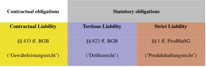
In the following the distinct mechanisms and ramifications arising from the three main liability constructs, which are depicted in Table2, will be discussed and the necessary and up-to-date references to case law to interpret and apply them correctly will be provided to lay the legal groundwork necessary for later discussions. In doing so, a self-contained and concise overview of these extensive areas of civil law is developed, thereby removing the requirement of prior knowledge of the subject matter on the part of the reader.
Table 2.Overview of the three main liability constructs for defective products
Liability for defective products
Contractual obligations Statutory obligations
Contractual Liability Tortious Liability Strict Liability
§§ 433ff. BGB §§ 823ff. BGB §§ 1ff. ProdHaftG
(‘Gewährleistungsrecht’) (‘Deliktsrecht’) (‘Produkthaftungsrecht’)
In essence, all statutory provisions of relevance to the discussions in this work are those of the special part of the law of obligations (‘Schuldrecht - Besonderer Teil’) and the Product Liability Act (‘Produkthaftungsgesetz’). There is however a caveat to that. For these sections are not self-contained but have to be interpreted in the broader context of the code due to provisions included by reference.
It will be shown that these distinct liability constructs are not mutually exclusive, but coexist and can be applied in parallel. An awareness and understanding of these liability mechanisms is therefore of paramount importance and ought to be incorporated into and influence all stages of research, product design and development.
3.1. Contractual Liability
relationship between the parties4 while the latter covers faulty conduct (‘Verschuldenshaftung’) as well as strict (as for there is no fault requirement) liability (‘Gefährdungshaftung’)5. They will be addressed in the above order.
Thus, before discussing matters of tortious product liability (‘deliktische Produzentenhaftung’) and strict product liability (‘Produkthaftung nach ProdHaftG’) attention shall be directed to contractual liability.
3.1.1. Requirements
For a contractual liability to attach the prerequisite of the existence of a valid sales contract between buyer and seller has to be satisfied. Depending on whether the relationship is “Business to Consumer” (B2C) or “Business to Business” (B2B) laws pertaining to purchase agreements (‘Kaufvertragsrecht’) or to contracts to produce a work (‘Werkvertragsrecht’) apply, for the B2C and B2B scenarios, respectively.
Typical contractual duties in a purchase agreement are listed in § 433 BGB and in § 631 BGB for a contract to produce a work.
3.1.2. Material and Legal Defects
§ 433 I 2 BGB states that “the seller must procure the thing for the buyer free from material and legal defects”. It shall be emphasized that in this context the term defect is subject to a wide interpretation.
As one would expect, § 434 I 1 BGB states that in order to be considered free of material defects the thing, upon the passing of risk (‘Gefahrenübergang’), has to be of the agreed quality. The legislator’s broad interpretation of the term defect however becomes apparent in § 434 I 2 BGB which specifies that, in case the quality has not clearly been articulated in the respective contractual agreement, the thing has to be “suitable for the use intended under the contract” (§ 434 I 2 No. 1 BGB) or it has to be suitable for the customary use and of the quality a reasonable buyer would expect from a product of this kind (§ 434 I 2 No. 2 BGB). The legislator goes on to further clarify that quality under § 434 I 2 No. 2 BGB includes expectations reasonably induced in the buyer by advertisement or public statements concerning product characteristics made by the seller, the producer or vicarious agents of either one (§ 434 I 3 BGB).
The product, on the other hand, is considered free of ‘legal defect’ if pertaining to the purchase third parties can either assert no rights at all or only assert such rights appropriated by the buyer in the underlying contractual agreement (§ 435 BGB)6. Klindt et al. [47] provide the example of a software that was sold even though it incorporates and uses proprietary libraries without the appropriate license. This would constitute a textbook example of a ‘legal defect’ of the product as the rights holder may bring actions against the buyer of said software product.
Klindt et al. [47] further elaborate on the particular nature of software defects liability. Even though the legal community widely accepts the fact that due to the intrinsically complex nature of software products an absolute absence of material defects cannot be achieved according to the prevailing opinion this shall not justify a deviation from the generally accepted and above stated definitions of what constitutes a product defect7.
4 Contractual obligations are “covered by some 570 paragraphs (§§ 241-811 BGB) of which the first 191 (§§ 241-432 BGB) refer to
problems common to all obligations. The remainder deal with specific contracts. They include sale and exchange (§§ 433-515 BGB), gift (§§ 516-34 BGB) which, in the civil law systems, is regarded as a contract), lease (§§ 535-97 BGB), basic rules of labor law (§§ 611-30 BGB) and contract of labor and services (§§ 631ff. BGB) and others. The law ofnegotiorum gestio(‘Geschäftsführung ohne Auftrag’) follows in § 677 BGB while unjustified enrichment (‘ungerechtfertigte Bereicherung’) is regulated by §§ 812ff. BGB” [46], p. 24
5 “The BGB devotes thirty paragraphs (not including § 835 BGB which was repealed) to the law of torts - and they form the
twenty-fifth title of the second book dealing with obligations. The term unerlaubte Handlungen is often used to cover the domain that Anglo-American lawyers would ascribe to ‘torts’ but the term used precisely is best understood to cover faulty conduct (Verschuldenshaftung). The wider term Deliktsrecht probably covers better liability that is both based on fault (proved or presumed) and is strict.” [46], p. 24
6 Furthermore, sentence 2 specifies that “it is equivalent to a legal defect if a right that does not exist is registered in the Land Register.”
For B2B scenarios the notion of material and legal defect is defined analogously in § 633 BGB. For the sake of brevity the following discussion will mainly consider B2C scenarios.
3.1.3. Is Software a Corporeal Object?
Furthermore, Klindt et al. [47] bring a seminal Federal Court of Justice decision to the reader’s attention. In a 2006 landmark decision 8 the BGH found landlord and tenant law (‘Mietrecht’) to be applicable to Application Service Providers (ASP) 9. Due to this judgment and the inherent similarities (as it pertains to the legal transactions involved) of ASP and Cloud Computing it is to be assumed that the latter is impacted analogously by the decision.
An important implication is that § 535 BGB on contents and primary duties of lease agreements can be applied to its full extent. Specifically, § 535 I 2 BGB imposes extensive duties on the lessor (i.e. the ASP in this case), most importantly the duty to maintain the leased property in a condition suitable for use by the lessee in conformity with the contract. This implies that the provider may be obliged to perform certain adjustments, e.g. install critical updates and patches and furthermore to keep the overall software up to date so as not to fail to maintain the system in a condition suitable to be used for the intended purpose outlined in the contractual agreement. For the time period of the lease agreement statutes of limitations (‘Verjährungsfristen’) pertaining to demands to remedy defects are suspended [47].
Further to this the court also found software to be a thing in terms of § 90 BGB for which depending on whether the goods were surrendered subject to a purchase or a lease agreement sales or tenancy laws are to be applied, respectively. Note that § 90 BGB states that “only corporeal objects are things as defined by law”, a definition that at first sight would exclude software products. However the court argued that for the software to be of any actual use it necessarily had to be materialized on some sort of storage medium thereby satisfying the corporeal object requirement. This is consistent with previous BGH decisions regarding the composition of software10.
3.1.4. Legal consequences of defects
The rights granted by the legislator to the buyer of a defective product are manifold (see, e.g. [48] for an exhaustive discussion of the matter).
§ 437 BGB states that the buyer may:
1. demand cure under § 439 BGB
§ 439 (‘Nacherfüllung’) on the cure of the defect can certainly be seen as a piece of rather buyer-friendly legislation.
In fact, the buyer can freely choose whether to have the defect remedied (i.e. have the thing repaired, ‘Nachbesserung’) or rather have a thing free of defects supplied (i.e. receive a new one, ‘Nachlieferung’). Note that in principle the buyer is free to choose either of said options regardless of the sellers preference (§ 439 I BGB) and that the seller is obliged to bear all expenses of the chosen cure (§ 439 II BGB).
The seller may only refuse the particular cure chosen by the buyer if it is unwarranted, i.e. if it would result in disproportionate expenses for the seller compared to the alternative cure (§ 439 III BGB).
2. revoke the purchase under §§ 440, 323, 326 V BGB
8 Cf. Judgment of the Federal Court of Justice of November 15th, 2006 - XII ZR 120/04. Source: NJW 2007, 2394.
9 “Application Service Provider: a company that provides software (as for e-mail or payroll accounting) that is accessible over the Internet
instead of being stored on individual computers —abbreviation ASP” Merriam-Webster.com. Merriam-Webster, n.d. Web. 21 Feb. 2017.
If the buyer set a deadline for the seller to cure the defect and said deadline has lapsed without success (§ 323 I BGB) or if special circumstances rendered the imposition of such a deadline dispensable (§§ 281 II, 323 II, 440 BGB) (e.g. because the seller “seriously and definitively refuses performance”, § 323 II No. 1 BGB or because the cure is impossible, § 326 V BGB) the buyer may rescind the purchase agreement (§ 437 No. 2 Alt. 1 BGB) given the defect is substantial (§ 323 V 2 BGB).
3. reduce the purchase price under § 441 BGB
§ 441 I 1 states that “instead of revoking the agreement, the buyer may, by declaration to the seller, reduce the purchase price” (§ 437 No. 2 Alt. 2, 441 I BGB). § 441 I 2 further specifies that “the ground for exclusion under § 323 V 2 does not apply”, i.e. the defect does not have to be substantial for the buyer to invoke the right to reduce the purchase price. The mere presence of a defect suffices.
4. demand damages under §§ 440, 280-283, 311a BGB
The buyer may also seek compensation for damages due to the defect (§§ 437 No. 3 Alt. 1, 440, 280, 281, 283, 311a BGB). Note that the defect has to be substantial for the buyer to be able to recover damages (§ 281 I 3 BGB).
5. demand reimbursement of futile expenses under § 284 BGB
If the buyer made expenditures in the reasonable expectation that the seller would supply the purchased object free of defects and these expenses become futile due to the seller’s breach of duty, the buyer can seek reimbursement of these futile expenses (§§ 437 No. 3 Alt. 2, 284 BGB).
3.1.5. Boundaries on the Exclusion of Contractual Liability
In light of the above considerations it may appear tempting to exclude or limit liability by resorting to contractual provisions. This subsection will explore the strict boundaries imposed by the legislator on such practices.
First of all, generally speaking, contracts come in a variety of shapes and forms. For the purpose of this analysis the crucial distinction to make appears to be the one between individually negotiated terms of contract (‘Individualvertrag’) on one hand and general terms and conditions (‘Allgemeine Geschäftsbedingungen’ -AGB) on the other hand. While the legislator imposes relatively few and very basic boundaries on the former (e.g. violation of morality (‘Sittenwidrigkeit’) as in § 138 BGB), the latter are heavily regulated (§§ 305ff. BGB) as will be shown in the following.
§ 305 I 1-2 BGB define general terms and conditions as
all contract terms pre-formulated for more than two contracts which one party to the contract (the user) presents to the other party upon the entering into of the contract. It is irrelevant whether the provisions take the form of a physically separate part of a contract or are made part of the contractual document itself, what their volume is, what typeface or font is used for them and what form the contract takes.
It is clear that in practice the vast majority of contracts will fall into this category, hence its importance. Furthermore, “contract terms do not become standard business terms to the extent that they have been negotiated in detail between the parties” (§ 305 I 3 BGB) and “individually agreed terms take priority over standard business terms” (§ 305b BGB).
to consistent decisions by the BGH merely ‘negotiating’ contractual provisions does not suffice, rather an act of bargaining is required11.
For general terms and conditions to be validly incorporated the contracting party needs to acknowledge and agree to them (§ 305 II BGB). Surprising and ambiguous clauses are void by law (§ 305c I BGB) and if doubts in the interpretation arise they are resolved against the user of the pre-formulated terms and conditions (§ 305c II BGB). The rules in §§ 305ff. BGB apply regardless of possible attempts “to circumvent them by other constructions” (§ 306a BGB).
The legislator severely limits the user’s ability to exclude liability. First and foremost, § 307 I BGB states that provisions “are ineffective if, contrary to the requirement of good faith, they unreasonably disadvantage the other party to the contract with the user. An unreasonable disadvantage may also arise from the provision not being clear and comprehensible.”
Furthermore, § 309 BGB explicitly forbids the “exclusion of liability for injury to life, body or health and in case of gross fault” (§ 309 No. 7 BGB) as well as “other exclusions of liability for breaches of duty” (§ 309 No. 8 BGB) - of particular relevance here those pertaining to defects in “contracts relating to the supply of newly produced things and relating to the performance of work” where provisions excluding liability for defects overall or in regard to individual parts are void by law as are those “limiting to the granting of claims against third parties or made dependent upon prior court actions” (§ 309 No. 8 aa) BGB).
It is also worth mentioning that the recent addition of § 309 No. 14 to the German Civil Code specifies that provisions mandating an attempt of Alternative Dispute Resolution (ADR) to have been undertaken and failed prior to the filing of a claim against the user are also explicitly forbidden12.
3.2. Tortious Product Liability
For the sake of this discussion the special part of the law of obligations (‘Schuldrecht Besonderer Teil’) can be thought of having two main pillars:
(i) ‘contractual obligations’ (‘vertragliche Schuldverhältnisse’) (ii) ‘statutory obligations’ (‘gesetzliche Schuldverhältnisse’)
of particular relevance to the matter at hand, the ‘law of unlawful actions’ (‘Recht der unerlaubten Handlungen’ or ‘Deliktsrecht’)
While implications of the former were discussed in the previous section, in this section the focus will be on the latter, also known as ‘the law of torts’. Broadly speaking, a tort is a civil wrong other than a breach of contract for which damages can be recovered.
3.2.1. The German Law of Torts, §§ 823-853 BGB
There are three ‘general provisions’ in the German law of torts, namely §§ 823 I, 823 II and 826 BGB, of which § 823 I is generally regarded as being the most significant. The sections read as follows:
§ 823
(1) A person who, intentionally or negligently, unlawfully injures the life, body, health, freedom, property or another right of another person is liable to make compensation to the other party for the damage arising from this.
(2) The same duty is held by a person who commits a breach of a statute that is intended to protect another person. If, according to the contents of the statute, it may also be breached without fault, then liability to compensation only exists in the case of fault.
11 Cf. Judgment of the Federal Court of Justice of March 20th, 2014 - VII ZR 248/13. Source: NJW 2014, 1725
12 § 309 No. 14 BGB as introduced by the amendment of the German Civil Code, effective February 26th, 2016, cf. BGBl I Nr. 9/2016,
§ 826
A person who, in a manner contrary to public policy, intentionally inflicts damage on another person is liable to the other person to make compensation for the damage.
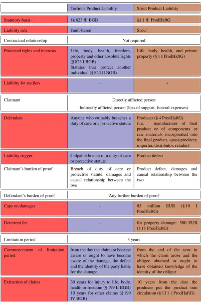
First of all it shall be emphasized that, contrary to specific product liability acts, the delict provisions of the BGB, i.e. §§ 823-853, are not specifically intended to address product liability matters but are general tools for the claimant to seek compensation for damages that arose from the infringement of one or multiple of the claimant’s absolute rights by a tortfeasor’s faulty conduct.
‘Absolute rights’ are ‘erga omnes’ (Latin for ‘towards all’) rights, i.e. “rights which can be interfered with by everyone and which can be asserted against everyone” ([46], p. 69).
In contrast, ‘relative rights’ would be rights that can only be asserted on the basis of an existing legal relationship, e.g. rights that can be asserted by one party against other parties it has entered into a binding contractual agreement with.
The most relevant delict provisions pertaining to product liability matters, i.e. § 823 I and § 823 II, will be analyzed in the following.
It shall be pointed out that § 826 is distinct in that it allows for the recovery of purely economic loss, provided that the damage was inflicted intentionally (i.e. willfully and ‘not just negligently’) and “in a manner
contra bonos mores” ([46], p. 15). The recovery of purely economic loss is not possible under § 823 I (it is though under § 823 II). Note however that the factual prerequisites of an intentional infliction that furthermore has to becontra bonos moreslimits the actual applicability of § 826 compared to §§ 823 I,II.
3.2.2. Fault-based Product Liability under Tort Law
§ 823 I BGB provides that damages arising from the intentional or negligent, unlawful injury to life, body, health, freedom, property or other absolute rights of another person are to be compensated by the wrongdoer.
Note that
1. The statute is applicable only to infringements committed by a person (physical or legal) to the detriment of another person’s rights or interests, provided they are one of the rights or interests explicitly listed by the statute or included by reference to the person’s ‘other (absolute) rights’, as discussed earlier.
2. No contractual or semi-contractual relationship between the parties is required.
3. Damages must arise from the wrongdoers faulty conduct (‘Verschuldenshaftung’), i.e. the conduct has to be willful/intentional (‘vorsätzlich’)13or negligent (‘fahrlässig’)14.
4. The conduct must furthermore be unlawful. According to the prevailing opinion this requirement is regularly met whenever a person’s absolute rights are infringed absent a legally recognized justification (‘Rechtfertigungsgrund’)15.
13 The definition of intention and negligence is provided by § 276 BGB which states that “the obligor is responsible for intention and
negligence, if a higher or lower degree of liability is neither laid down nor to be inferred from the other subject matter of the obligation, including but not limited to the giving of a guarantee or the assumption of a procurement risk. The provisions of § 827 and § 828 apply with the necessary modifications.” § 276 I BGB.
14 “A person acts negligently if he fails to exercise reasonable care.” § 276 II BGB.
15 The determination of unlawful conduct is not as straightforward as it may appear to the non-jurist. Markesinis points out that “acts ...
5. There must be an adequate causal link between the claimant’s damages and the defendant’s conduct, either by
(a) an active act (‘Aktives Tun’)=⇒ascertained to by applying the ‘conditio sine qua non’ formula ; or by
(b) an act of omission (‘Unterlassen’) =⇒ ascertained to by applying the ‘conditio cum qua non’ formula.
Liability arising from acts of omissions evidently deserve careful consideration in the area of products liability. For it may be argued that in the ordinary course of events, an infringement of protected rights or interests by the manufacturer due to negligent or intentional omission is more likely than due to active wrongdoing.
In German law, one of the most fertile sources of the development of liability for omissions and, indeed, of the whole law of tort, was the development of the idea that a preceding dangerous (or potentially dangerous) activity or state of affairs should give rise to a duty of care. From this idea, the courts slowly but steadily developed the famous Verkehrssicherungspflichten. The term Verkehrssicherungspflicht is not easy to translate. But its meaning could be summarized by saying that whoever by his activity or through his property establishes in everyday life a source of potential danger which is likely to affect the interests and rights of others, is obliged to ensure their protection against the risks thus created by him.([46], p. 86.)
The notion of duty of care pertaining to § 823 I and its ramifications shall therefore be examined in the following subsection.
3.2.3. Duty of Care (§ 823 I BGB)
The following duties of care have been established by German case law
1. Liability for defective design (‘Konstruktionsfehler’)
Duties of care are relevant from the very beginning of a product’s development cycle. For the manufacturer has to design the product such that to his best abilities and under reasonable economic feasibility constraints, no unreasonably unsafe or dangerous product with respect to the current scientific and technological knowledge will be placed on the market.
This implies careful design of the product in appreciation of its intended use and user group, most importantly whether the product is designed for professional or consumer use. The manufacturer is also expected to anticipate and take into account the (potentially improper) use of its product outside the intended scope and by users other than those it was originally intended for and marketed to if he knew or ought to have known that such scenarios were conceivable.
The manufacturer’s duties of care also extend to the careful selection of and the exercise of reasonable quality control measures pertaining to components produced by subcontractors.
2. Liability for defects in manufacture (‘Fabrikationsfehler’)
Presuming the absence of design defects, defective products may still result from irregularities in the manufacturing process itself, e.g. due to human error or defective machinery.
In this context it is important to emphasize that the manufacturer is not liable for ‘outliers’ (‘Ausreißer’), i.e. single defective products, provided he undertook reasonable and adequate efforts to avoid them or at least to detect them and hinder the afflicted products from leaving the manufacturer’s ‘sphere of control’. As shall be explained in Section 3.3, the ‘outlier-defense’ can however only be invoked to exculpate oneself from tortious liability whereas the manufacturer will still be held strictly liable under ProdHaftG.
3. Liability for defective instruction (‘Instruktionsfehler’)
The manufacturer is obliged to clearly warn from dangers arising from the use of its product, especially if used as intended and if the danger is not immediately discernible. Depending on the level of danger and the foreseeability of misuse or improper use giving rise to said danger, the duty to make users aware may also expand to encompass use cases outside the product’s intended use.
Warnings have to be articulated clearly and unambiguously and, depending on the severity of the danger, be further emphasized and highlighted. There is however no duty to warn from obvious dangers of which the user knew or ought to have known. Warning labels therefore tend to be used more ‘conservatively’ in comparison to e.g. the United States and bizarre warning labels such as the infamous16‘do not dry pets in microwave’ are virtually unheard of.
The manufacturer may also be obliged to amend the original warnings and/or instructions provided with the product if new facts come to light that would call for such an action.
4. Liability arising from a breach of organizational duty (‘Verletzung der Organisationspflicht’)
The manufacturer is generally obliged to implement organizational measures and procedures so as to avoid the establishment of sources of potential dangers to the best of his ability. This duty overlaps with other duties of care imposed onto the manufacturer, be they statutory or established by case law.
5. Liability for development risk (‘Verletzung der Produktbeobachtungspflicht’)
As already stated above under the section discussing the manufacturer’s liability for defective instructions, the manufacturer’s duties do not end once the product has been placed on to the market. In fact, the manufacturer shall monitor for and react to new evidence pertaining to possible dangers arising from use of the product.
Case law established that, under certain conditions, this duty also encompasses products by other parties (e.g. accessories) that, when used in combination with the product may give rise to dangers.
Depending on the severity of the newly discovered danger the manufacturer may even be obliged to proceed with a product recall.
3.2.4. Burden of Proof
In German tort law - in particular pertaining to §§ 823 I,II BGB - an alleviation of the burden of proof has been established by case law. For the courts acknowledged it would regularly amount to an undue burden (or even be infeasible) for the claimant to prove the alleged tortfeasor’s fault (i.e. to establish that the conduct that led to the damages was intentional or negligent), as would be required following a strict interpretation of the law.
It has therefore been established that providing so-calledprima facie(Latin for ‘at first sight’) evidence for the alleged tortfeasor’s fault and the causal relationship to the damages claimed suffices as long as no
16 According to what is reported to be an urban legend, an elderly woman unwittingly killed her cat in an attempt to dry the pet that
compelling contradictory explanation or evidence surfaces [49].
Pertaining to tortious product liability in particular, said alleviations eventually culminated into a full shift of the burden of proof (‘Beweislastumkehr’) in favor of the claimant. According to both case law upheld and established by the BGH and prevailing scholarly opinion said reversal in product liability matters is just, for the burden on the claimant would otherwise be disproportionate, especially in face of today’s complex and intricate (distributed) manufacturing processes [46,49–51].
It may therefore be argued that tortious product liability, which as a matter of principle is based on faulty conduct, has effectively been tilted towards strict liability [46,49,50].
3.2.5. Statute of Limitations and Caps on Damages
The general limitation period of the BGB, i.e. three years under § 195 BGB, applies and according to § 199 I BGB begins with the end of the year in which the claim arose (§ 199 I No. 1 BGB) and “the obligee obtains knowledge of the circumstances giving rise to the claim and of the identity of the obligor, or would have obtained such knowledge if he had not shown gross negligence” (§ 199 I No. 2 BGB). It may be interrupted according to § 204 BGB on the suspension of limitation periods as a result of the prosecution of rights.
There are some exceptions however imposing longer but absolute (as in they begin on the date on which the act, breach of duty or other event that caused the damage occurred irrespective of the particular manner in which they arose and the knowledge thereof) limitation periods of either thirty years for injury to life, body, health or freedom (§ 199 II BGB) or ten years for most other claims (§ 199 IV BGB). The reason for claims eventually becoming statute-barred is to provide legal certainty for all parties involved.
As for caps on damages recoverable through tortious product liability, there are none in the German law of torts. This constitutes a major differentiating factor with respect to other potentially competing constructs for the recovery of compensatory damages, e.g. various specific strict liability statutes such as ProdHaftG.
Also note that German law does not allow for punitive damages17 and similarly rejects the concept of class action lawsuits18.
3.2.6. Protective Statute (§ 823 II BGB)
Claims under § 823 II for compensatory damages can be brought if they arose from a person’s (i.e. the -alleged - wrongdoers) breach of a statute that is intended to protect another person. The claimant however must prove that the violated statute awarded him protection from the specific act, breach of duty or other event that was perpetrated on him and gave rise to the damages being claimed ([46], p. 888).
The importance of § 823 II arises from the fact that it remarkably expands § 823 I by including by reference various other statutes. By doing so it allows to recover damages such as purely economic losses that could not be recovered through § 823 I. It is therefore often referred to as the ‘small general clause’ of the German law of torts [46,49,50].
3.3. Strict Product Liability
Despite some alleviations pertaining to the burden of proof in tortious product liability matters have been established by case law (seeSection3.2.4), the fundamental distinction between fault-based liability under tort law and strict liability under special acts still holds.
17 German law (and virtually all civil law countries) does not allow for punitive damages. “German courts and legal literature emphasize
that punitive damages are not only unknown to German law, but are contrary to German public policy. Thus, to this day, American punitive damage awards are not enforced in Germany.” [52], pp. 107-108. Cf. also [53–55].